the Creative Commons Attribution 4.0 License.
the Creative Commons Attribution 4.0 License.
 | 15 Sep 2020
Mind the gap – Part 2: Improving quantitative estimates of cloud and rain water path in oceanic warm rain using spaceborne radars
Pavlos Kollias
Ranvir Dhillon
Katia Lamer
Marat Khairoutdinov
Daniel Watters
The intrinsic small spatial scales and low-reflectivity structure of oceanic warm precipitating clouds suggest that millimeter spaceborne radars are best suited to providing quantitative estimates of cloud and rain liquid water paths (LWPs). This assertion is based on their smaller horizontal footprint; high sensitivities; and a wide dynamic range of path-integrated attenuations associated with warm-rain cells across the millimeter wavelength spectrum, with diverse spectral responses to rain and cloud partitioning.
State-of-the-art single-frequency radar profiling algorithms of warm rain seem to be inadequate because of their dependence on uncertain assumptions about the rain–cloud partitioning and because of the rain microphysics. Here, high-resolution cloud-resolving model simulations for the Rain in Cumulus over the Ocean field study and a spaceborne forward radar simulator are exploited to assess the potential of existing and future spaceborne radar systems for quantitative warm-rain microphysical retrievals. Specifically, the detrimental effects of nonuniform beam filling on estimates of path-integrated attenuation (PIA), the added value of brightness temperature (TB) derived adopting radiometric radar modes, and the performances of multifrequency PIA and/or TB combinations when retrieving liquid water paths partitioned into cloud (c-LWPs) and rain (r-LWPs) are assessed. Results show that (1) Ka- and W-band TB values add useful constraints and are effective at lower LWPs than the same-frequency PIAs; (2) matched-beam combined TB values and PIAs from single-frequency or multifrequency radars can significantly narrow down uncertainties in retrieved cloud and rain liquid water paths; and (3) the configuration including PIAs, TB values and near-surface reflectivities for the Ka-band–W-band pairs in our synthetic retrieval can achieve an RMSE of better than 30 % for c-LWPs and r-LWPs exceeding 100 g m−2.
- Article
(7792 KB) - Companion paper
- BibTeX
- EndNote


Warm rain is precipitation that originates from non-ice-phase processes usually in clouds whose tops lie below the atmospheric freezing level. Warm rain is the dominant mechanism for precipitation formation over the tropical oceans outside the Intertropical Convergence Zone, accounting for slightly more than 30 % of the total rain amount and 70 % of the total rain area in the 30∘ S–30∘ N belt (Lau and Wu, 2003). It has been shown that warm precipitation significantly contributes to moistening and heating of the lower troposphere through latent heat release over most of the tropical and subtropical oceans, thus partially counteracting the low-level cooling induced by stratiform rain (Kodama et al., 2009). In addition, it can impact the organization of shallow convection (Savic-Jovcic and Stevens, 2008; Wang and Feingold, 2009; Yamaguchi and Feingold, 2015; Zhou et al., 2017). There is also evidence that warm rain impacts cloud lifetime (Paluch and Lenschow, 1991) and even causes changes in cloud regimes; Stevens et al. (1998) noted that, in the presence of strong precipitation, shallow stratocumulus clouds tend to dissipate. Since these direct and indirect mechanisms ultimately affect the global radiative budget and the hydrological cycle (Takahashi et al., 2017; Testik and Barros, 2007), it is important to accurately monitor and quantify the oceanic warm-rain variability and improve its representation in large-scale models (Stephens, 2005; Dufresne and Bony, 2008).
Global observations of warm rain (Lau and Wu, 2003; Liu and Zipser, 2009; Berg et al., 2010; Kodama et al., 2009) rely on spaceborne radar observations (Battaglia et al., 2020a): the W-band (94 GHz) cloud profiling radar (CPR) operated from CloudSat (Tanelli et al., 2008) and the Ku–Ka dual-frequency (13.8 and 35.5 GHz) precipitation radar (DPR) on board the Global Precipitation Measurement (GPM) mission core observatory (Skofronick-Jackson et al., 2017) and, before 2014, on the Ku-band precipitation radar (PR) operated on the Tropical Rainfall Measuring Mission (TRMM; Kummerow et al., 1998). A number of studies (e.g., Schumacher and Houze, 2003; Berg et al., 2010; Rapp et al., 2013; Lamer et al., 2020) have suggested that none of these spaceborne sensors can describe the entire spectrum of precipitation since, depending on their operational wavelength, such radars are sensitive to precipitation that is either light (e.g., CloudSat CPR) or moderate and heavy (e.g., TRMM PR), and depending on their pulse length they may be of limited use near the surface (⪅500–1000 m height) due to surface clutter and low vertical resolution (≥250 m).
NASA's CloudSat CPR offers excellent sensitivity (better than −27 dBZ) combined with the smallest footprint (1.4 km) among existing spaceborne radar missions. Thus, the CPR measurements are used as a reference for the occurrence of light precipitation and drizzle over the oceans (Stephens et al., 2010; Ellis et al., 2009) assuming that a sensitivity of −15 to −25 dBZ is required to detect drizzle (Kollias et al., 2011).
In Part 1 of our studies (Lamer et al., 2020), we focused on spaceborne radars' ability to detect and locate the presence and boundaries of low-level clouds and precipitation and determined that surface clutter limits the CloudSat CPR's ability to observe true cloud base in ∼52 % of the cloudy columns it detects and true virga base in ∼80 %, meaning the CloudSat CPR often provides an incomplete view of even the clouds that it does detect. Vertical profiling of such cloud systems down to the closest few hundred meters to the surface with a vertical resolution of 250 m or less has been deemed feasible with the next generation of radars, given that they operate with an interleaved shorter pulse (Kollias et al., 2007).
The adoption of aforementioned sampling strategies could lead to a substantial improvement in our ability to map the vertical structure of warm rain. However, quantitative retrievals using single-frequency radar measurements remain challenging (Lebsock and Su, 2014; Battaglia et al., 2020b). Retrievals of the profile of liquid water content (Lebsock and L'Ecuyer, 2011; Leinonen et al., 2016; Awaka et al., 2016) mainly rely on radar reflectivity profiles. Since reflectivities are sensitive only to the largest and most reflective particles, they provide information only on the rain component. When single-frequency measurements are used, the retrieval of rain profiles is inherently affected by large uncertainties related to the a priori assumptions about the rain microphysics and its vertical variability. For instance, in the majority of retrievals, a constant-with-height intercept parameter and an exponential drop size distribution (DSD) are assumed. The prospect of using multiwavelength radar measurements can provide additional information about the vertical structure of cloud and precipitation and thus relax such assumptions (Battaglia et al., 2020c, a). Using CloudSat observations, Rapp et al. (2013) and Wang et al. (2017) suggest that the onset of precipitation occurs for the cloud liquid water path exceeding values ranging from 150 to above 300 g m−2; the c-LWP is then expected to grow with the r-LWP (see Fig. 6 in Lebsock et al., 2011). The cloud affects the radar signal only by attenuating the measured reflectivities; since attenuation amounts to ca. 0.8 to 4 and 12.0 dB kg−1 m2 of column-integrated cloud liquid content when moving from 35 to 94 and 220 GHz only at the highest frequencies there is a tangible effect. Furthermore, the challenge of detecting the cloud base height (Lamer et al., 2020) limits our ability to constrain the vertical extent of the cloud liquid.
Additional constraints to the cloud component come from auxiliary measurements that may include visible optical thicknesses during the daytime and/or path-integrated attenuations (PIAs) over the ocean and/or co-located microwave brightness temperatures. Cloud water dominates the visible optical depth with the rain mode only contributing up to 5 %–10 % depending on the details of the DSD (Lebsock and L'Ecuyer, 2011). PIA techniques rely on the contrast between observed surface radar reflectivity under cloud-free conditions and under rain and associate this difference with the attenuation produced by the total water mass in the column. Brightness temperature (TB) corresponding to oceanic warm-rain cells is warmer than the clear-sky background due to the additional emission of cloud and precipitation (Wentz and Spencer, 1998; Lebsock and Suzuki, 2016). Lebsock and Suzuki (2016) quantified the typical sensitivities of 94 GHz PIAs and TB on the total water path to 0.08 K g−1 m2 and 0.008 dB g−1 m2 when small values of water paths are considered, with decreasing sensitivities with increasing water paths. They argued that since in the case of CloudSat the PIA precision of 0.16 dB is much better than the 4 K precision of TB, then PIAs can potentially achieve a much better retrieval uncertainty, on the order of 20 g m−2 (compared to 50 g m−2) at small water paths.
All the aforementioned integral constraints can substantially improve the estimates of c-LWPs and r-LWPs; however, they also have drawbacks. Visible optical thicknesses have collocation issues and may be affected by 3D effects; PIA estimates and TB measurements are often too noisy at small liquid water paths (LWPs) and strongly affected by nonuniform beam filling (NUBF; Kozu and Iguchi, 1999; Battaglia et al., 2020b; Wentz and Spencer, 1998; Lebsock and Suzuki, 2016) associated with the considerable spatial inhomogeneity of warm rain (Lamer et al., 2019).
The relative contribution of cloud and rain particles to the total attenuation depends on the frequency, with the cloud component becoming increasingly important both in absolute magnitude and relatively to the rain component with increasing frequency (e.g., see Fig. 2 of Battaglia et al., 2014). As the radar frequency increases, the size of the small raindrops that contribute the most to attenuation decreases (e.g., the most efficient ones are those of a 1.2, 0.48 and 0.2 mm radius at 35, 94 and 220 GHz, respectively). These frequency-dependent scattering properties underpin any remote-sensing-based technique for the separation of the cloud and rain component. Besides being essential in retrieval techniques, the partitioning between rain and cloud remains an important frontier in improving understanding of the autoconversion process.
This paper focuses on the quantification of warm oceanic cloud and rain water content using spaceborne radars. It aims to
-
discuss the reliability of existing measurements and algorithms and, in the process, identify existing gaps (Sect. 2) and
-
assess the potential of the future generation of radar observing systems to bridge these gaps, specifically determining (Sect. 3)
-
the impact of different footprints on nonuniform beam-filling effects and
-
if integral constraints for cloud and rain water paths can be improved using (1) radiometric radar modes, (2) different radar frequencies and (3) combinations of both types of measurements; these quantities are key in constraining profiling algorithms, and their accurate and precise retrieval is conditio sine qua non for any quantitative warm-rain characterization.
-
Conclusions are provided in Sect. 4.
Quantitative estimates of warm rain are currently produced from CloudSat and GPM observations. For CloudSat, CPR reflectivity profiles and auxiliary data from 2B-GEOPROF are first used to produce a cloud classification in order to identify pixels of warm rain and then exploited to provide profiles of liquid water content (including the separation between cloud and rain). The 2C-PRECIP-COLUMN algorithm utilizes measurements of the near-surface radar reflectivity and an estimate of the PIA to determine the actual incidence of precipitation. The classification of liquid precipitation into convective, stratiform or shallow types is then performed by the 2C-PRECIP-COLUMN algorithm (Haynes et al., 2009; Smalley et al., 2014) based on the vertical structure of reflectivity. In the absence of a reflectivity value of 0 dBZ or greater above the freezing level, the precipitation is classified as shallow.
Two sophisticated algorithms are relevant for warm rain: the 2C-RAIN-PROFILE (Lebsock and L'Ecuyer, 2011) and the 2B-CWC-RVOD (Leinonen et al., 2016) products. The algorithms produce rain rates as low as 0.001 mm h−1. In contrast to 2C-RAIN-PROFILE, which is based upon CloudSat radar reflectivities and PIA, the 2B-CWC-RVOD product also includes optical depths derived from the Moderate Resolution Imaging Spectroradiometer (MODIS) on the Aqua A-train satellite (L’Ecuyer and Jiang, 2010).
For GPM, the level-2A Ku, Ka and dual-frequency precipitation radar (DPR) products provide a warm-rain flag (flagShallowRain) and estimates of rain-rate profiles (Awaka et al., 2016). Warm rain is identified within a vertical profile where the storm top height is more than 1 km below the freezing level (Iguchi et al., 2010). Furthermore, the warm rain is classified as isolated or nonisolated depending upon the horizontal size of the system. In this study, these two categories have been grouped together. Due to the large differences in sensitivity (−29 dBZ vs. +12 dBZ for the CloudSat CPR and the GPM DPR, respectively), it is reasonable to expect differences in their respective climatology of oceanic warm rain (Liu and Zipser, 2009). Another important factor to consider is the difference in sampling, with the CPR providing only nadir-pointing observations, while the DPR provides measurements of a 250 km swath.
A CloudSat-based global climatology of occurrence and amount of oceanic warm rain constructed using observations collected between January 2007 and December 2010 is shown in Fig. 1a and c. The analysis is restricted to ocean where warm rain is mainly present and because PIA estimates over ocean are much better constrained thanks to the highly predictable ocean surface backscattering signal (Haynes et al., 2009). A number of features are apparent from Fig. 1. Warm rain is widely distributed over the tropics and the subtropics where the freezing level is located between 4 and 5 km. The occurrence and amount of warm rain are most prominent in the intertropical convergence zone in the east Pacific, where congestus clouds and shallow cumulus clouds below trade inversions coexist with deep convective systems (Johnson et al., 1999). The oceanic warm-rain climatology exhibits zonal variability with higher occurrence at warmer sea surface temperatures (SSTs) that coincide with ascending branches of the Walker circulation. On the contrary, lower occurrences are found near the eastern continental boundaries where colder SSTs and large-scale subsidence result in higher lower-tropospheric stability that limits the vertical extent of oceanic clouds and their ability to produce rain.
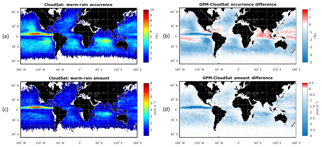
Figure 1Occurrence and amount of global warm rain at the ground as determined by CloudSat (data from January 2007 to December 2010) and GPM (data from July 2014 to June 2018), using a spatial resolution of . The CloudSat (GPM) results were produced using the 2C-PRECIP-COLUMN and 2C-RAIN-PROFILE (2A-DPR) products. (a, c) Global occurrence and amount of warm rain as observed by CloudSat. (b, d) Difference in occurrence and amount between GPM and CloudSat.
A similar climatology is derived using GPM DPR observations over the period July 2014 to June 2018. The differences between the GPM and the CloudSat climatology of warm-rain occurrence and amount are shown in Fig. 1b and d. In general, GPM underestimates both occurrences and amounts. In order to gain insights into the factors contributing to the observed differences in the ocean warm-rain climatology, an example of coincident observations from the CloudSat CPR and the TRMM PR is shown in Fig. 2. Note that the same features can also be found when comparing the CloudSat CPR with the GPM DPR, since Ku-band TRMM and GPM radars have similar performances in terms of sensitivities and resolution. A number of warm precipitating cloud systems are clearly identified by the CloudSat CPR (reflectivity in Fig. 2a) thanks to its excellent sensitivity and finer resolution. Note that the freezing level is located at about a 4 km altitude (magenta line in Fig. 2a). The Ku-band TRMM radar (see reflectivity in Fig. 2b) has a much coarser horizontal resolution and lower sensitivity and can detect only the three most heavily precipitating cells of the scene where the CloudSat CPR is affected by strong attenuation (two-way W-band PIA well exceeding 20 dB, Fig. 2c). The differences in sensitivity and horizontal resolution between current W-band and Ku- and Ka-band systems imply that TRMM-like and GPM-like spaceborne radars generally struggle to identify occurrence of drizzle and light warm rain – let alone estimate its intensity – which is well detected by the CloudSat CPR. Conversely, high-intensity warm rain, associated with strong attenuation of the CloudSat CPR signal, is likely to be better quantified by TRMM-like and GPM-like radars.
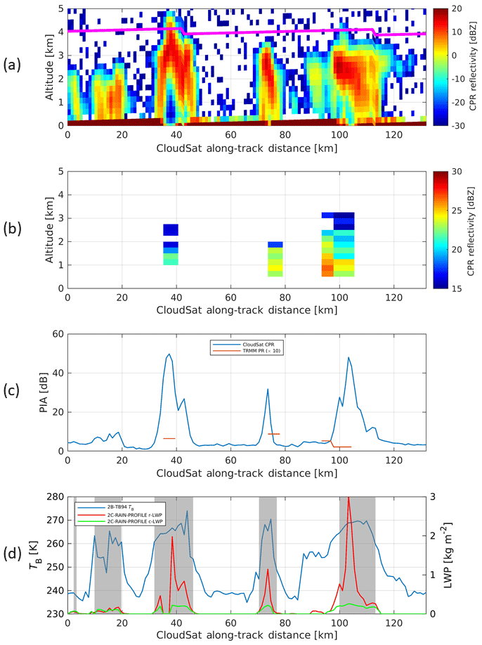
Figure 2Coincident CloudSat and TRMM satellite overpasses over oceanic warm-rain cells (2 January 2008, 07:46:46–07:47:05 UTC). (a) Vertical profile of CloudSat radar reflectivities with the magenta line indicating the freezing level height. (b) TRMM PR reflectivities. (c) CloudSat and TRMM (multiplied by 10) two-way PIASRT's (PIASRT denotes PIA via the surface reference technique). (d) CloudSat brightness temperature. The shaded regions correspond to profiles of warm rain as identified by 2C-PRECIP-COLUMN.
There are a few tropical regions where GPM overestimates warm rain. This can be either associated with an inconsistency between the two classification algorithms (e.g., GPM warm-rain classification may misclassify shallow nonisolated pixels that tend to occur in regions associated with deep convective systems; Funk et al., 2013) or related to the different resolutions of the GPM and CloudSat radars. The majority of GPM warm-rain cells (55 % of the occurrences corresponding to more than 22 % of the warm-rain-covered area) corresponds to a single GPM pixel. The single-GPM-pixel resolution is 25 km2 and that of CloudSat is 1.5 km2. Thus, horizontally narrow warm rain with sufficient radar reflectivity to be detected by both sensors can potentially occupy an area 16 times larger in the GPM climatology than it will in the CloudSat climatology. A simple 1D rescaling of the occurrences from the CloudSat 1.1 km along-track resolution to a GPM-like 5.5 km scale accounting for the reduced GPM sensitivity (with a fixed detection threshold assumed to be 0.02 mm h−1, the threshold for warm rain from the 5 km GPM DPR product) shows that this effect (Fig. 3) explains part of the GPM overestimation in the occurrence statistics. Despite not properly accounting for the 2D averaging, it is clear that the footprint of the instrument (and the minimum detection level) has a large impact on the determination of warm-rain occurrences.
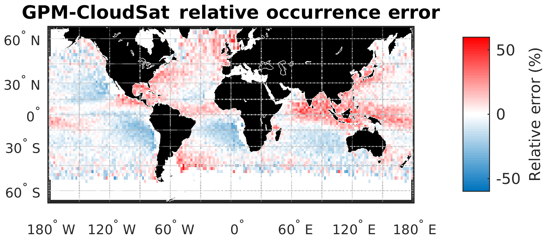
Figure 3Simulated effect on warm-rain occurrences produced by averaging the 1.1 km along-track CloudSat rain rates to a 5.5 km scale and using a 0.02 mm h−1 detection threshold on the 5.5 km averaged rainfall. This figure shows the enhancement (positive values) or reduction (negative values) in percentage compared to the CloudSat occurrences.
In addition to the aforementioned challenges related to sensitivity and footprint, recent studies (Christensen et al., 2013; Mace et al., 2016) concluded that it is very challenging to properly constrain either the cloud or the precipitation properties using only single-frequency radar measurements. To further support this, density histograms of the cloud liquid water path (c-LWP) and rain liquid water path (r-LWP) derived from the 4 years (from 2007 to 2010) 2C-RAIN-PROFILE (x axis) and the 2B-CWC-RVOD (y axis) CloudSat products are shown in Fig. 4. The relationship between the cloud and rain water path estimates in these products is very weak. The use of different a priori assumptions and the use of different input measurements to retrieve these parameters can explain the observed differences. However, one is left wondering what is the true distribution of the c-LWP and r-LWP and what is their relationship.
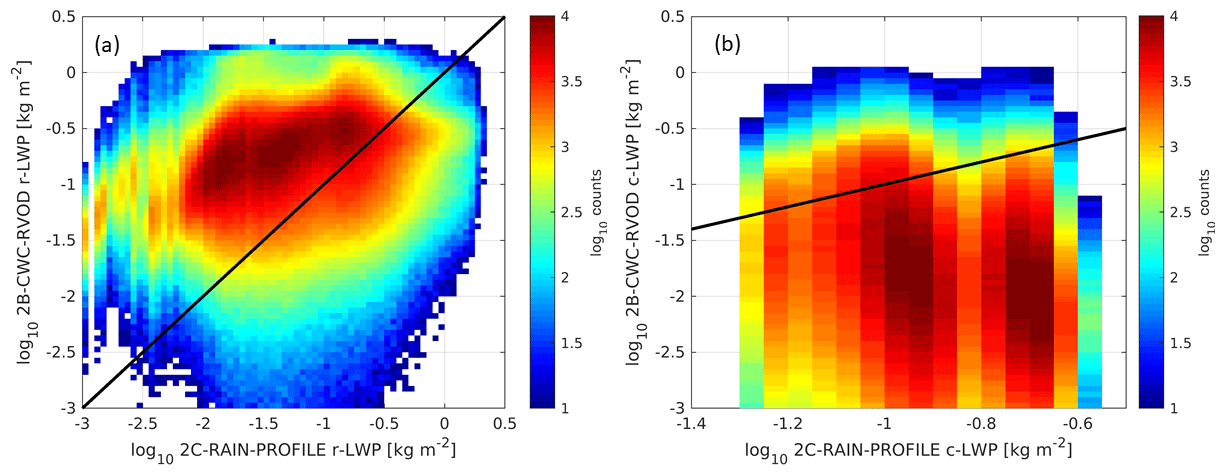
Figure 4Comparisons of the (a) rain LWP (r-LWP) and (b) cloud LWP (c-LWP) during warm rain (from 2007 to 2010, daytime only) for two CloudSat retrieval algorithms, 2B-CWC-RVOD and 2C-RAIN-PROFILE. Black lines correspond to the 1:1 line; evidence of correlation between the values obtained from the two CloudSat products is minimal.
When considering precipitating warm clouds it is clear that future observing systems need to outperform A-Train-like observations in order to better constrain precipitation processes. In addition, the scientific community is currently undertaking several notional studies to assess the potential of different multifrequency radar concepts (Battaglia et al., 2020a), with the core effort at NASA being in preparation of the Aerosol and Cloud, Convection and Precipitation (ACCP) mission, following the recommendation of the National Research Council Decadal Survey for Earth Sciences (The Decadal Survey, 2017). Advances in radar technology enable new research avenues, with three aspects of particular relevance for warm-rain studies.
-
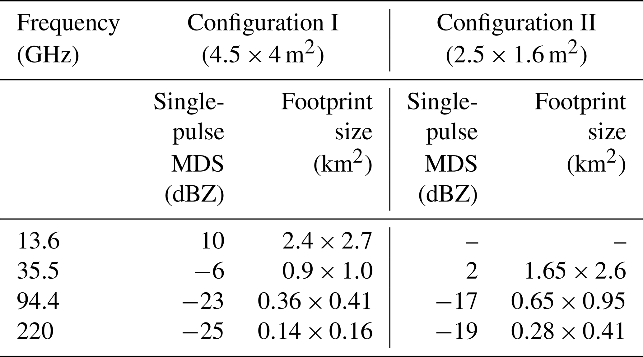
The next generation of spaceborne radars should achieve better sensitivities and finer vertical and horizontal resolutions (see Table 1 for two specifications currently under consideration). This work focuses on evaluating the impact of the reduction in horizontal resolution on quantitative estimates.
-
Multifrequency radars including channels within the G-band (Battaglia et al., 2014; Cooper et al., 2018; Roy et al., 2018; Battaglia and Kollias, 2019) are now plausible candidates for constellation concepts. Clearly different frequencies are tailored to different targets, with higher (lower) frequencies more suitable for observing clouds (precipitation) because of their better sensitivity (reduced attenuation), as demonstrated in Fig. 2.
-
Radars with radiometric modes can provide perfectly antenna-matched TB, with the possibility of fully exploiting the combination of active and passive measurements. An example is provided by the CloudSat brightness temperature product (2B-TB94 available at http://www.cloudsat.cira.colostate.edu/data-products, last access: 27 August 2020; see details in Mace et al., 2016) derived from processing the noise floor data contained in the 1B-CPR data product. For the case study shown in Fig. 2 the CloudSat TB (panel d) is well correlated with the presence of the cells, with an enhancement of TB values, compared to the cold oceanic background at ∼240 K, induced by cloud and rain emission like that observed in Advanced Microwave Scanning Radiometer (AMSR) channels at a similar frequency (Eastman et al., 2019). Interestingly, TB seems to produce a quicker response than the PIA to the presence of the rain cells. This is due to two reasons. First, visually, with the scale of values shown in the y axis of panels c and d, it is much easier to see a change in TB on the order of 1 K than a change in PIA of 0.1 dB (which both correspond to a water path of roughly 12.5 g m−2). Second, CloudSat TB values are computed by averaging along-track using a 5-pixel boxcar window, so they have a coarser resolution than that of the PIA.
Table 1Summary of specifications for two radar configurations currently under study: one with a very large antenna and one with a smaller antenna. A flying altitude of 400 km and a range resolution of 500 m are assumed. MDS is minimum detection signal.
3.1 Methodology
A forward simulator framework using cloud-resolving model simulations as input is used to test the impact of the horizontal resolution of the different radar configurations and to assess the potential of a multifrequency radar system (with or without radiometric mode). Two cloud field conditions are evaluated (one with freezing levels around 4.9 km and the other with freezing levels around 3.4 km), and a total of 12 different radar configurations were tested with three different footprints for each frequency (as tabulated in Table 2) which span the range of values currently employed or expected in the near future.
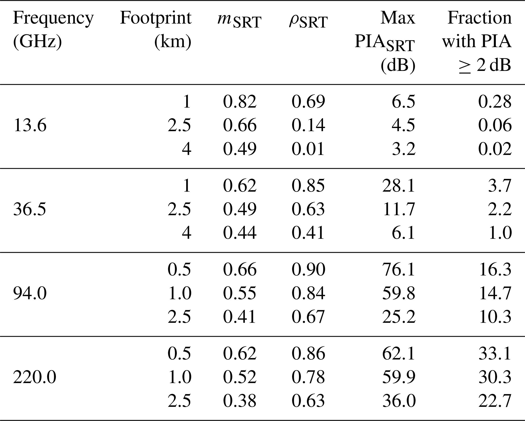
Table 2NUBF effect on PIA estimates based on the surface reference technique. For all footprints an along-track integration length of 500 m is assumed. In the last column the fraction of profiles with PIA exceeding 2 dB is referenced to the number of profiles having a c-LWP or r-LWP exceeding 10 g m−2 at a 0.5 km resolution.
3.1.1 RICO simulations
The simulations are based on data collected during the Rain in Cumulus over the Ocean (RICO) field study. RICO was a comprehensive field study of shallow cumulus convection which was located in the winter trade winds of the northwestern Atlantic ocean, just upwind of the islands of Antigua and Barbuda. An overview of the experiment is provided in Rauber et al. (2007). The focus of RICO was on the statistical character of the cloudy boundary layer, particularly on the characterization of precipitation in shallow cumulus. The cloud-resolving model used in this study is version 6.11.2 of the System for Atmospheric Modeling (SAM) described by Khairoutdinov and Randall (2003). Double-moment (Morrison et al., 2005) microphysics was used with a prescribed concentration of cloud droplets of 100 cm−3. The horizontal doubly periodic domain size was 57.6 km × 57.6 km with horizontal grid spacing of 100 m, while the vertical grid had 120 levels with the domain top at 4.8 km and constant 40 m grid spacing.
Two simulations have been performed. The setup of the first simulation closely follows the setup used in the study by vanZanten et al. (2011). The second simulation was for drier conditions, more characteristic of the midlatitudes than the subtropics. There is no straightforward way to scale the soundings and forcing profiles to accomplish that, so a very simple procedure was used. The original sea surface temperature of 299.8 K and the initial temperature of the sounding were reduced by 9.8 K. The water vapor sounding and prescribed large-scale vapor tendencies were scaled by a factor that was obtained to keep the relative humidity at the first model level constant. The other profiles, such as the horizontal wind and subsidence rate were not changed. As the result of the procedure, the freezing level moved from around 4.9 km down to a 3.4 km height. Each simulation was run for 2 d with a time step of 2 s.
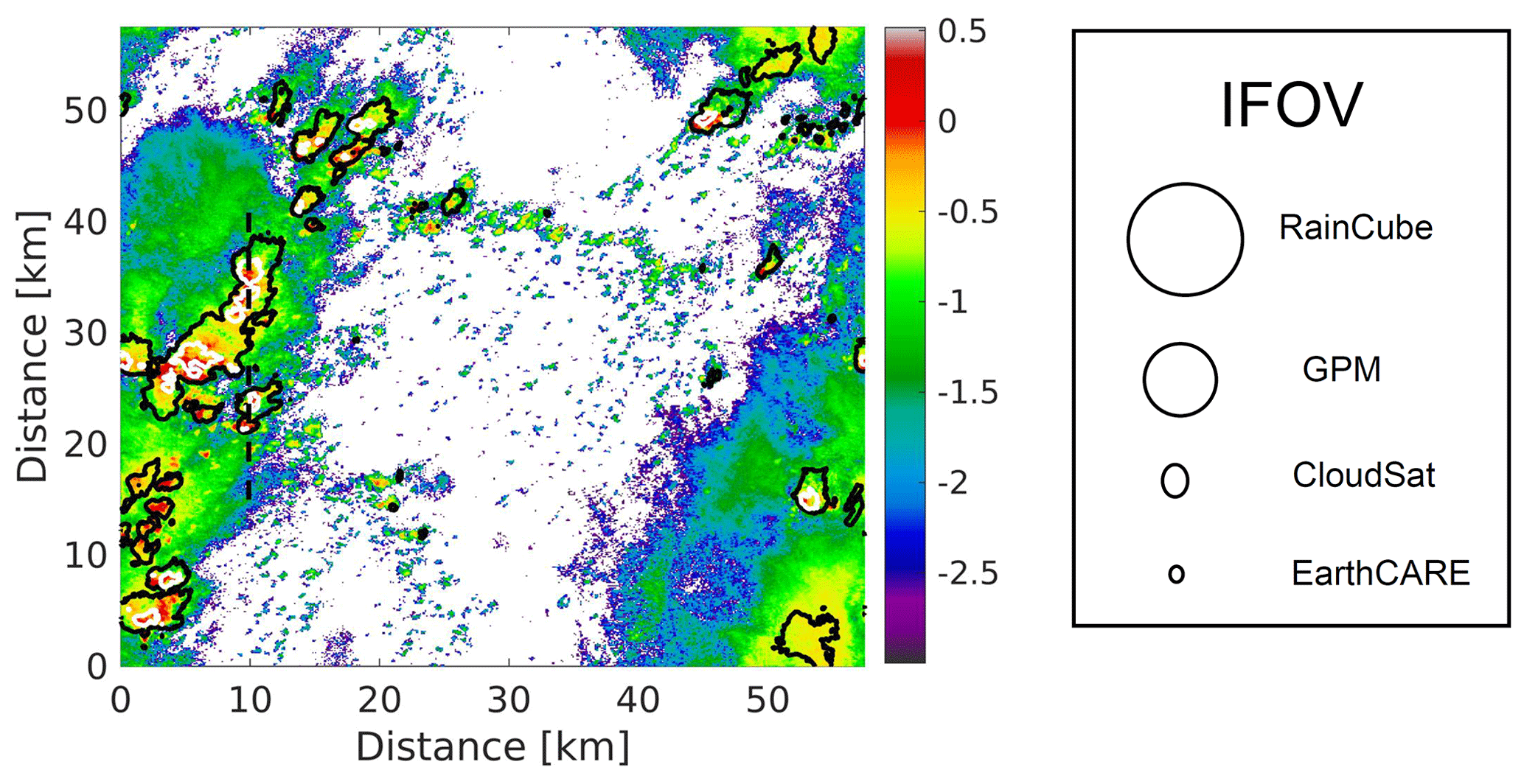
Figure 5 shows one scene (out of the 65 considered in this study) illustrating the low-freezing-level simulations with the colors modulated by the total integrated c-LWP and the contour lines showing the r-LWP equal to 0.1 and 0.5 kg m−2, (black and gray lines). Instantaneous fields of view (IFOVs) of planned and operated spaceborne radars are shown for reference on the right-hand side.
3.1.2 Forward radar simulator
Four steps are followed in order to produce radar observables from the model output.
-
Scattering properties of the medium are computed at the fine model resolution. Gas attenuation is computed according to the model from Rosenkranz (1998). Scattering properties of cloud droplets and raindrops are computed via Mie theory (e.g., see Lhermitte, 1990). An exponential drop size distribution is assumed for rain with m−4 (Marshall and Palmer, 1948) whereas a Gamma distribution with μ=3 with an effective radius increasing from 3 to 15 µm from cloud base to cloud top according to Bennartz (2007) is adopted. The impact of the Marshall and Palmer assumption is discussed later.
-
The scattering properties are used as input of the radar forward model developed in Hogan and Battaglia (2008) for computing the attenuated and unattenuated reflectivity profiles (but with the multiple-scattering flag turned off) and of an Eddington approximation code (Kummerow, 1993) for computing TB.
-
A surface echo is added. The surface normalized backscattering cross section, σ0, is computed as a function of the 10 m wind speed and the sea surface temperature following Wu (1990). For the computation of TB, surface emissivities are computed according to ocean Fresnel models.
-
The results produced in steps 2 and 3 are convolved with the radar range weighting functions with a top-hat pulse with a 500 m range resolution (see Lamer et al., 2020) and two-dimensional Gaussian antenna patterns with different instantaneous fields of view. Along-track integration of 500 m is carried out.
-
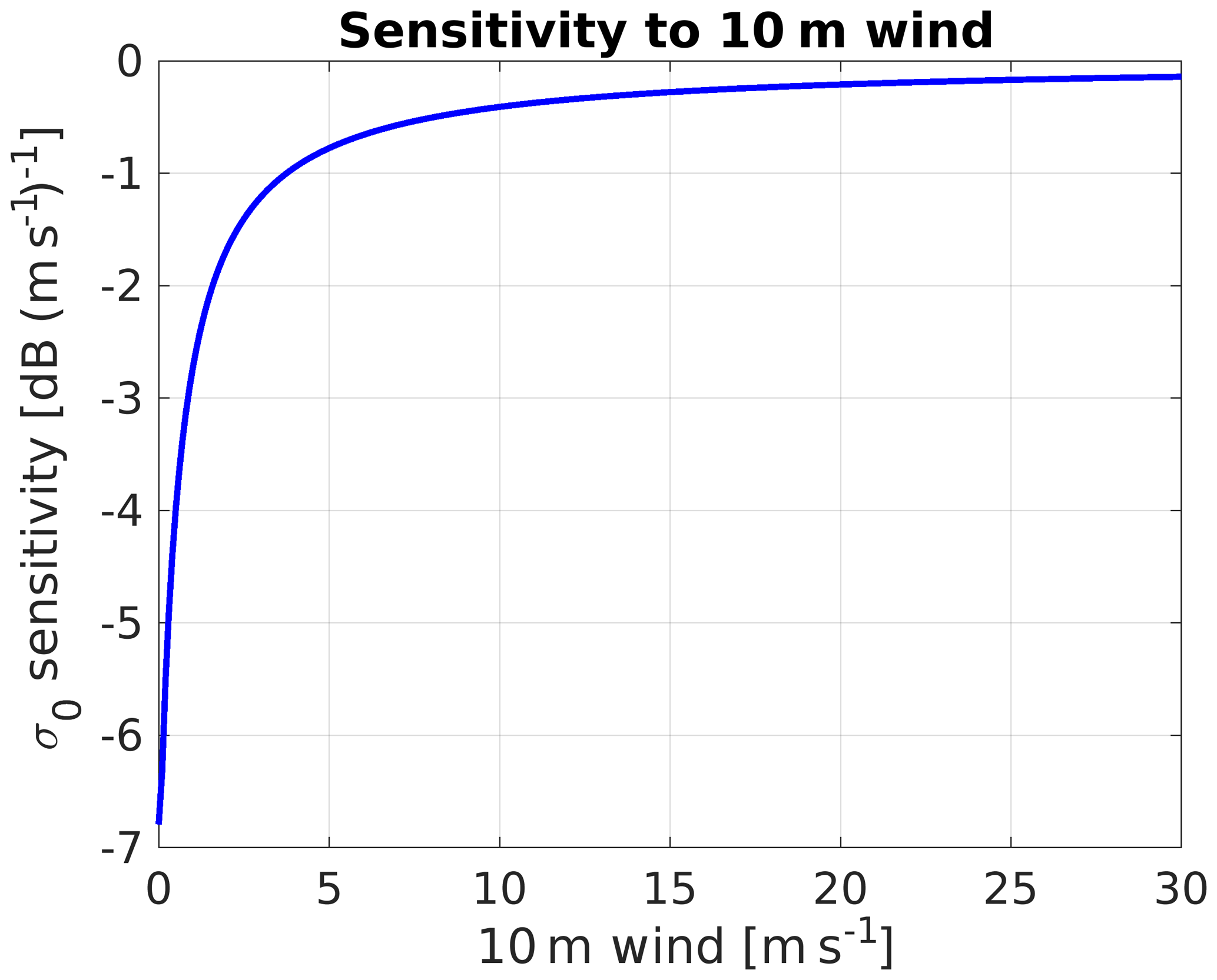
Random noise with a zero mean and 2 K (0.7 dB) standard deviation is added to the TB values and the PIAs, while reflectivity noise is computed using the dependence on signal-to-noise ratio (SNR) and averaging pulses described in Hogan et al. (2005). Note that, as shown in Leinonen et al. (2017), the uncertainty in the PIA is dominated by the uncertainty in the clear-sky σ0 and not by the uncertainty in the surface return (unless for cases close to full attenuation) which, at a high SNR and for CloudSat configuration, amounts to 0.17 dB (Lebsock and Suzuki, 2016). Leinonen et al. (2017) articulate that the uncertainty in the clear-sky σ0 can be estimated from the standard deviation of the observed clear-sky surface cross sections, with an average value of 0.24 dB for CloudSat so that the total PIA precision is estimated to be 0.29 dB. In reality this is an optimistic assumption because the clear-sky σ0 is likely more uncertain, especially if there are no clear-sky observations in the vicinity of the cloudy or rainy profile, which occurs e.g., when continuous stratocumulus cloud decks are present. In addition, even if such calibration points are available, winds are likely to change in the presence of precipitation due to local circulation (e.g., this feature is evident in the SAM simulations, not shown). σ0 has a strong sensitivity to the 10 m wind speed (Fig. 6), whereas the sensitivity to SST is very weak (<0.08 dB K−1, not shown). Therefore with 7–10 m s−1 wind (which are characteristic values in our simulations), an uncertainty of 1 m s−1 in the wind speed induces an uncertainty of roughly 0.4–0.6 dB in σ0 (with much worse results obtained for lower wind speeds). Therefore we generally think that a PIA precision of 0.7 dB is more appropriate to be assumed in our discussion. Similarly nadir emissivity sensitivities are on the order of 0.2–0.3 % m−1 s at all frequencies here considered. A 1 m s−1 uncertainty propagates into a maximum 0.6–1 K uncertainty in the TB values.
-
Since the sensitivity improves proportionally to the antenna gain, the single-pulse minimum detection signal (MDS) of each configuration is obtained by scaling the values provided in Table 1 for each frequency according to the scaling of the antenna footprint area. Forward-simulated reflectivities below the MDS are removed.
3.1.3 Example of simulated radar observables
Figure 7 indicates the integrated cloud and rain LWP, the brightness temperature TB, and the path-integrated attenuation PIA along the dashed black line drawn in Fig. 5. The integrated measurements are shown for different horizontal resolutions (model 0.1 km and radar 1 and 4 km) and for different radar frequencies (Ku-, Ka-, W- and G-band). The horizontal transect of the cloud and rain LWP indicates the presence of two clusters of shallow precipitating clouds with the first one having the majority of its water in cloud-size droplets and the latter having the majority of its water in rain-size particles. Each cell is approximately 5 km wide and exhibits considerable variability with two to three cores spaced by 1.5–2 km. The integrated LWP is shown in the original model resolution and for two different radar footprints (1 and 4 km). Noticeably, the 1 km radar footprint is able to preserve the shallow precipitation spatial variability, while the 4 km footprint results in considerable smearing of the warm-rain spatial distribution. This is consistent with the discussion in Sect. 2. TB clearly reacts to the emission of the precipitating clouds which warm the cold oceanic background (Eastman et al., 2019). When increasing frequency, the nadir ocean emissivity and the atmospheric gas optical thickness (mainly due to water vapor) rise, thus causing a significant warming of the baseline clear-sky TB. This reduces the contrast between clear-sky and rainy cells, thus making TB measurements less useful. On the other hand, optical thicknesses of the precipitating columns (which are driving the TB warming) also increase with frequency, thus making the high-frequency channels the most sensitive to the presence of rain. For instance, Ku-band TB values have a low baseline and a potentially large dynamic range, but only a few kelvins of enhancement are produced in this scene because of the low sensitivity of the Ku-band extinction to cloud and rain (see Battaglia et al., 2020a). Vice versa the W-band baseline TB values are already quite warm due to a high ocean surface emissivity; furthermore they are strongly affected by the amount of water vapor in the atmosphere, with significantly lower clear-sky baselines for environments with a lower freezing level (e.g., ∼235 K for this and, similarly, for the scene shown in Fig. 2 compared to ∼255 K for the scenes with the highest freezing level heights). TB values at 220 GHz (not shown) are already saturated in clear-sky conditions and are therefore not considered further in this paper.

Figure 7(a) Integrated cloud and liquid water path along the cross section shown in Fig. 5 at the native model resolution and when accounting for different footprint sizes, as indicated in the legend. (b) Brightness temperatures for different frequencies and footprint sizes as indicated in the legend. Random noise with a standard deviation of 2 K is added to the measurements. A nadir-looking geometry is assumed. (c) Two-way hydrometeor PIAs computed simulating SRT (surface reference technique) observations for different frequencies as indicated in the legend. Red, green, blue and magenta correspond to the Ku-, Ka-, W- and G-band, respectively.
For the same cross section, vertical profiles of cloud and rain water content and reflectivities are shown in Fig. 8. The two rain cells located around 23 and 35 km are well profiled by all frequencies, but the configurations with the largest footprints (panels b and d) tend to fatten their structures. The increased level of attenuation at higher frequencies is clearly highlighted by the reduction in the surface return (panels e and f); at 220 GHz, the surface return and the 1.5 km lowest rain disappear below the MDS, corresponding to the heavily precipitating core at 35 km.
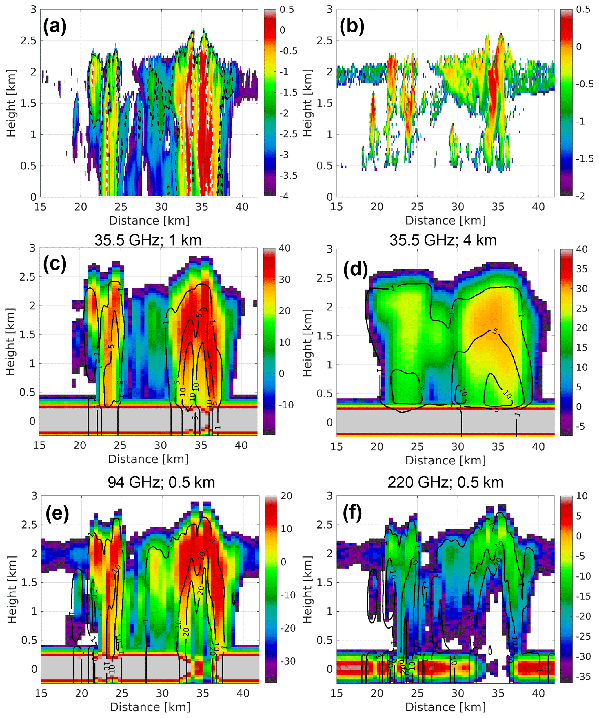
Figure 8(a) Vertical profile of r-LWC (rain liquid water content) for the cross section corresponding to the black line shown in Fig. 5 at the model resolution (100 m); the dashed black and white lines correspond to Dm equals 0.5 and 1.5 mm, respectively. (b) Vertical profile of c-LWC (cloud liquid water content) for the same cross section. The units of the color bar for both (a) and (b) corresponds to log 10 of LWC in grams per cubic meter; so for instance −1 means 0.1 g m−3. (c–g) Simulated vertical profiles of reflectivities (color bar units: dBZ) for bands and horizontal resolutions as indicated in the text at the top each panel. Black lines correspond to contour levels of the antenna-weighted PIA from the top of the atmosphere.
3.2 Results
3.2.1 Impact of instrument footprint
Warm precipitating clouds are naturally very inhomogeneous as clearly highlighted in Fig. 5. This inhomogeneity and their inherent 3D structure is very challenging when considering spaceborne observations, with the instrument footprints naturally convolving (thus smoothing) the natural variability of the rain microphysics fields. For instance the sharp peaks in the c-LWP and r-LWP at the 100 m model native resolution are already reduced when moving to 1 km footprints and completely washed out when moving to 4 km (Fig. 7a). Similar effects can be seen in TB values and PIAs (e.g., compare lines with the same colors and different styles in Fig. 7b and c) and also in the reflectivity profiles with rainy cells appearing less intense but with larger horizontal extent for the coarser-horizontal-resolution radar configurations (compare Fig. 8c and d).
NUBF effects are particularly detrimental when considering estimates of (two-way) PIA via the surface reference technique (hereafter designated PIASRT) and in the implementation of attenuation corrections for measured reflectivities within profiling algorithms (Durden, 2018, and reference therein). The PIASRT is derived by contrasting the surface return under rainfall and the surface return under clear-sky conditions (Nakamura, 1991; Meneghini et al., 2015). In equations
whereas the “true” PIA is obtained via averaging the integrated attenuation along each direction Ω within the footprint, pia(Ω):
where the integrals are extended to the full antenna pattern and G represents the antenna gain. If pia(Ω) is constant across the footprint then PIASRT=PIA, but in the presence of NUBF PIASRT always underestimates the true PIA, as a direct consequence of the concavity of the exponential function. This is clearly demonstrated in Fig. 9 for a Ka-band having a footprint of 1 and 4 km (panels a and b, respectively). Note the presence of negative values for PIASRT (y axis) in correspondence to small true PIAs due to the injection of noise in their estimates. The radar footprint can impact the PIA estimates in two different ways:
-
It can lead to considerable underestimation of the PIA due to NUBF effects (i.e., the spatial extent of the cloud covers only a fraction of the effective radar footprint that is the result of the instantaneous field of view and of the along-track integration). This effect is amplified for larger radar footprints (see departure from the 1:1 line in Fig. 9).
-
The range of the true PIA value decreases when coarser footprints are adopted due to the convolution with the broader two-way antenna gain function. As a result of the smaller measured PIA values, the relative error introduced by the measurement error increases. Thus the fraction of useful PIA measurements strongly increases with greater frequencies and with smaller footprints (see last column in Table 2).
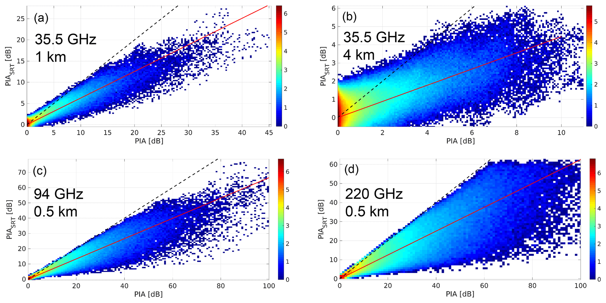
Figure 9Illustrating the impact of NUBF on estimate of the hydrometeor PIA via the surface reference technique: density scatterplot of hydrometeor PIA vs. PIASRT for the whole dataset of RICO simulations for Ka-band radars with footprint of 1 km (a) and 4 km (b) and for footprints of 0.5 km at 94 GHz (c) and 220 GHz (d).
Similar results are found at the other frequencies and are summarized in Table 2 where the slope coefficient of the fitting line (mSRT), the correlation (ρSRT) and the maximum value of the PIASRT's are reported. With the same footprint, the NUBF effect tends to be more and more acute with increasing frequencies. For current configurations like for the CloudSat CPR or the GPM Ka, the value of mSRT is significantly lower than 1. It is clear that proper corrections must be applied. While for the GPM DPR, studies are focused on identifying the pixels mostly affected by NUBF by using a combination of normal- and high-sensitivity scans (with flags introduced in the “Trigger” module; see Mroz et al., 2018) and on implementing corrections (Seto et al., 2015); to our knowledge, no mitigation is currently planned for warm-rain retrievals in the CloudSat algorithms currently in operation (Lebsock and L'Ecuyer, 2011; Leinonen et al., 2016). The same applies to the EarthCARE CPR (which is less affected, having a footprint substantially smaller) algorithms (Mason et al., 2017), now in preparation. A possible solution would be to identify regions highly affected by NUBF by producing PIASRT estimates at a much higher temporal frequency than cloud measurements (which is possible thanks to the typically higher SNR of the surface) and using the along-track PIA gradient as a proxy for NUBF (something similar is currently envisaged for the Doppler NUBF correction; e.g., see Kollias et al., 2014). The estimated gradient of PIASRT's could be used to partially correct for the bias. Figure 10 shows the relationship for a 94 GHz radar with a 0.5 km IFOV. There is still quite some spread around the median value (black line), as expected from the highly nonlinear impact of NUBF on PIASRT's (e.g., see example in Mroz et al., 2018). For larger footprints the spread of the biases around the median tends to increase (not shown). Most of the nonlinearities are expected to be particularly acute in the presence of footprints with considerable empty fractions. Future work should investigate the role of ancillary visible or infrared collocated images or of scanning or push-broom configurations with oversampled footprints to better quantify the footprint empty fraction.
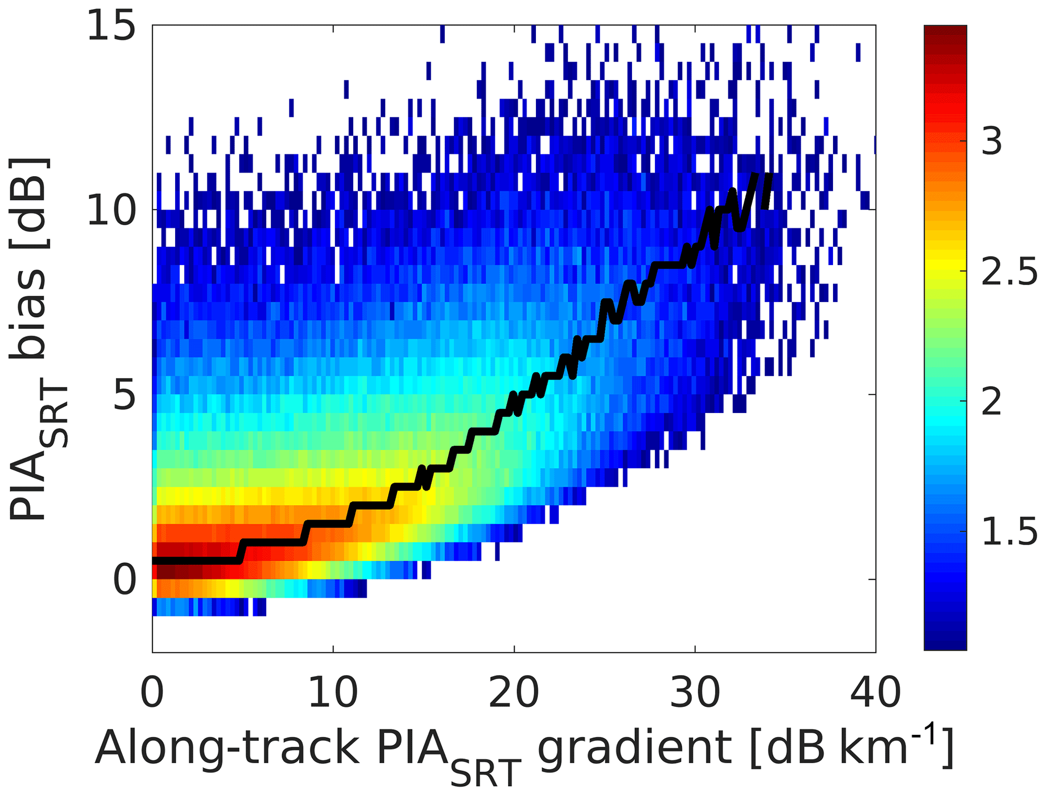
Figure 10Density plot of PIASRT bias (with respect to the true PIA) as a function of the absolute value of the along-track PIASRT gradient for the entire dataset of simulations. A configuration for an EarthCARE-like configuration is considered (94 GHz radar with a 0.5 km IFOV). The black line corresponds to the modal values of the biases for a given absolute value of the PIASRT along-track reflectivity.
3.2.2 Value of radiometric measurements vs. PIAs
In order to better assess the value of TB a simple scenario is considered, with the inclusion in the environment of the case study of Fig. 5 of a cloud layer at roughly 2 km and a rain layer underneath with increasing c-LWP and r-LWP values. The corresponding brightness temperatures for cloud-only (crosses) and rain-only (lines) conditions are plotted in Fig. 11. Different microphysics with exponentially distributed DSDs are considered for the rain. In addition to the Marshall and Palmer configuration we have added another configuration with a constant intercept of m−4 which is labeled as “Cumulus” since it resembles the one labeled with the same name in Lebsock and L'Ecuyer (2011). In addition the SAM model actually adopts a two-moment scheme where rain concentration and rain water content are both predicted (Morrison et al., 2005); such a scheme is approximated by a power law fit of the form , where Λ is the slope parameter in reciprocal meters and RWC is the water content in kilograms per cubic meter (and it will be referred to as “MO05”). From these plots the different response of the different frequencies is immediately clear: while the 13.6 GHz never saturates for an LWP smaller than 5 kg m−2, the 36.5 and 94 GHz saturates at different c- and r-LWPs. The sensitivity of TB to a change in cloud and rain LWPs is illustrated in Fig. 11b. The sensitivity to cloud is generally smaller than to rain, but such a difference becomes increasingly smaller with increasing frequencies, similarly for the differences between different rain microphysics. This is a direct consequence of the dependence of the extinction per unit mass on the characteristic size of the DSD (see Fig. A6 in Battaglia et al., 2020a).
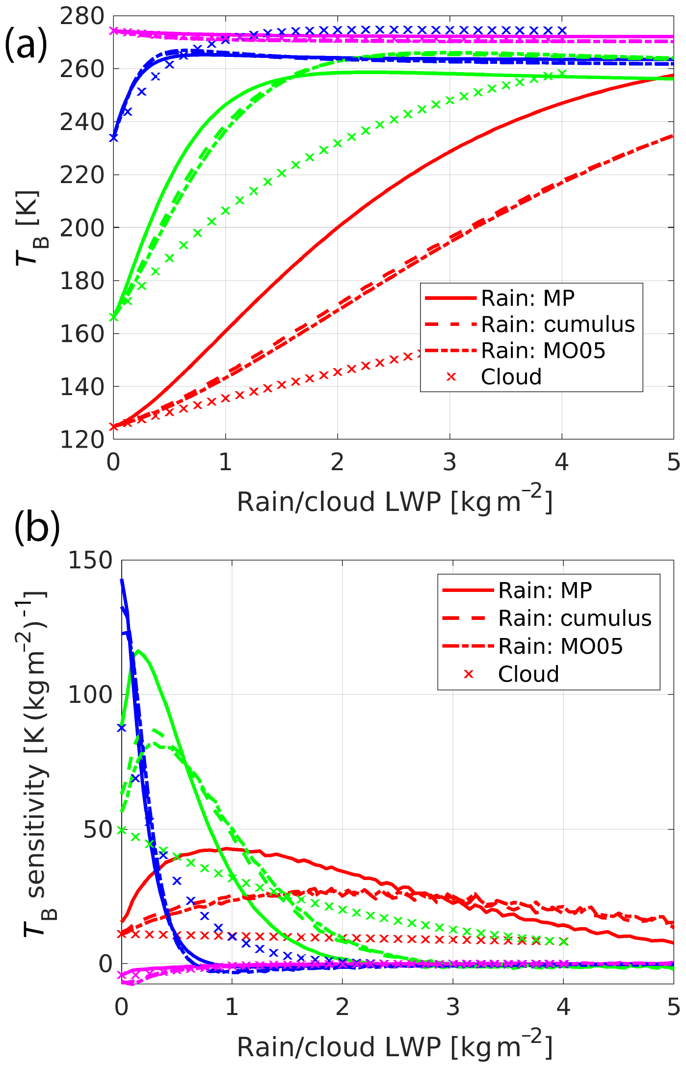
Figure 11TB (a) and TB sensitivity (b) as a function of the c-LWP and r-LWP for a simple scenario with cloud-only and rain-only conditions. Different microphysics schemes are considered for rain (see text for details). Red, green, blue and magenta lines correspond to 13.6, 36.5, 94 and 220 GHz, respectively.
The SAM simulation can reach very low cloud and rain LWPs (down to 10−4.5 and 10−5.5 kg m−2, respectively). An indication of how the two quantities covary when considering quantities averaged over footprints on the order of 1 km is provided by the color image in Fig. 12. Figure 12 further illustrates where PIA and TB can be useful as constraints for retrievals. In order to gauge the relevance of PIA and TB measurements, the mean values of ΔTB (defined as the enhancement of the TB values with respect to their clear-sky reference values) and PIAs in correspondence to different pairs of r-LWPs and c-LWPs binned logarithmically within their range of variability have been computed. A threshold of 0.7 dB for hydrometeor PIAs and of 2 K for ΔTB values has been used to roughly identify regions where those signals are sensitive to variations in c-LWPs and r-LWPs. The corresponding contour lines are shown in Fig. 12 for PIAs (dashed) and ΔTB values (continuous lines) for the different frequencies (different colors). We can make the following remarks.
-
Ka- and W-band ΔTB values and PIAs (see green and blue curves) are potentially very useful, as is G-band PIA. Ku-band PIA appears effective only for heavily precipitating clouds (i.e., r-LWP ≥400 g m−2). The inclusion of increasing frequencies increases the retrieval potential towards smaller values of the c-LWP, but, even when considering the G-band, integral constraints are useful only for c-LWPs and r-LWPs exceeding roughly 30 and 15 g m−2, respectively.
-
For any given frequency, TB is generally useful for smaller cloud and/or rain content compared to PIAs (if a precision of 2 K and 0.7 dB is assumed for TB and PIAs, respectively). For instance at 35 GHz for nonraining (raining) clouds, TB values are certainly useful for all instances of c-LWP >60 g m−2 (r-LWP >20 g m−2), but PIAs are useful only when c-LWP >350 g m−2 (r-LWP >100 g m−2). W-band (Ka-band) PIAs seem to have the same (slightly better) potential as Ka-band (than Ku-band) TB values.
-
TB tends to saturate at larger LWPs than the corresponding PIAs (see also Fig. 2). The dynamic range of TB values (defined as the difference between saturated and background TB) is constantly reducing with increasing frequency (because of the increase in the ocean nadir emissivity and the water vapor optical thickness). At the G-band (not shown) it becomes so small that TB values are practically of no use.
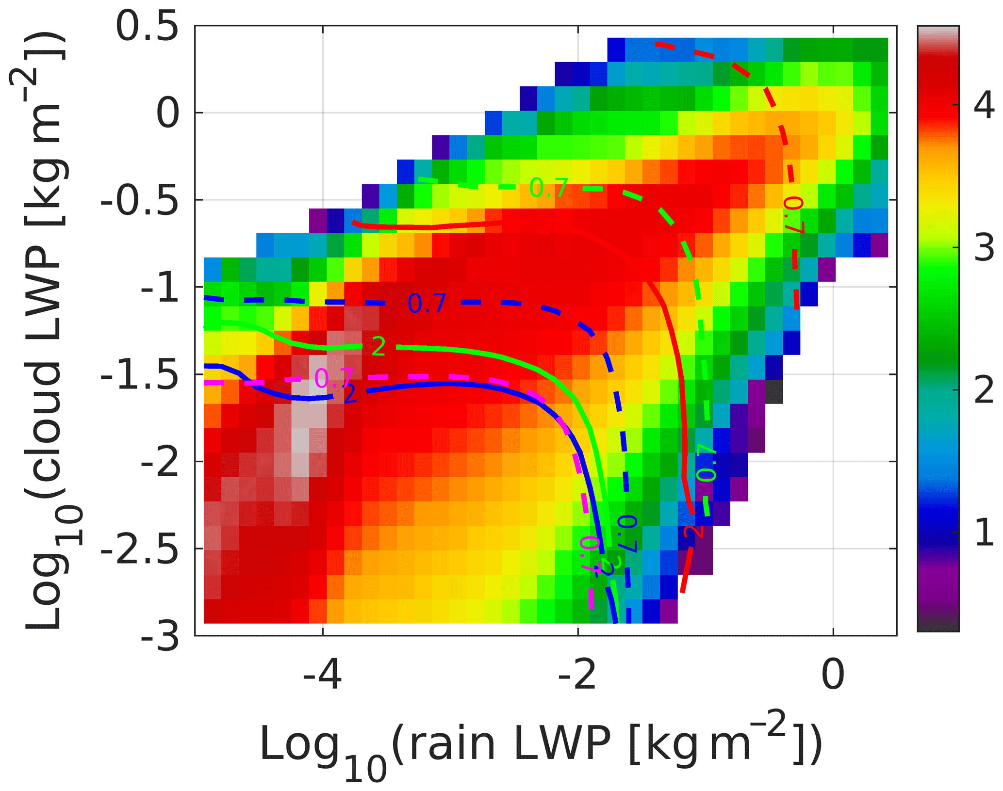
Figure 12Distribution of r-LWPs vs. c-LWPs with log 10 of the occurrences modulated by the color bar. Footprints of 1 km are used for all instruments. The continuous lines (unless otherwise labeled) correspond to where TB exceeds the background TB by 3 K, whereas dashed lines correspond to where the hydrometeor PIAs exceed 1 dB. Red, green, blue and magenta lines correspond to 13.6, 36.5, 94 and 220 GHz, respectively.
3.2.3 Potential of multifrequency retrievals of c-LWPs and r-LWPs
Here we want to investigate which frequency and which variable combination is more effective for retrieving column-integrated cloud and rain liquid water paths. The retrieval methodology is based on an ensemble Kalman smoother approach described by Grecu et al. (2018). The large database of RICO simulations is used to produce statistical relationships between observations and the state variables. Here the vector of unknowns is , while the vector of measurements can include both PIASRT's and TB values and/or reflectivities measured at the “closest-to-the-surface” clutter-free bin; thus yobs=[TB…Zns…PIA…], which can contain multiple frequencies and/or multiple observables. Note that near-surface reflectivities, when multifrequency observations are available, have been suggested as variables with good potential to provide constraints on integral quantities (Durden, 2018).
Given a vector of observations yobs, the retrieved vector of unknowns is computed as
where is a subset of the simulated observations of the training database within a normalized distance, δ (see Eq. 4), from yobs of less than 1 and is the corresponding state variables. The operator 〈 〉 indicates the mean operation across the subset. The normalized distance between the observation vector and the j element of the subset of is defined as
where σk is 2 K for TB and 1 dB for PIAs and depends on the SNR for Zns according to formula A9 in Hogan et al. (2005).
Absolute bias and root mean square errors for different combinations of observables at different frequencies with matched footprints of 1 km are plotted in Fig. 13. It is clear that Ka- and W-only retrievals perform poorly but with the W-band (Ka-band) performing better for the cloud (rain) component. Combining single-frequency PIAs and TB values (circles) certainly improves the retrieval, but it is the combination of two frequencies that definitely improves simultaneously c-LWPs and r-LWPs, with the Ka–W combination performing better than the W–G combination (compare cyan and magenta circles). The inclusion of near-surface reflectivities also produces a significant improvement in the performances of both the c-LWPs and the r-LWPs (see dashed lines). The inclusion of the G-band in addition to the Ka and W seems to only marginally improve results (compare dashed cyan and black lines). Note that LWPs are expressed in logarithmic units, thus RMS differences of 0.1, 0.2 and 0.3 correspond to fractional errors of , and , respectively. So for instance the Ka-band–W-band pair achieves the best retrieval performances with an RMSE of better than 30 % for c-LWPs and r-LWPs exceeding 100 g m−2. Similar conclusions (not shown) can be drawn when 2.5 km footprints are used.

Figure 13Bias (a, c) and RMSE (b, d) in retrievals of c-LWPs (a, b) and r-LWPs (c, d) in log 10 units for the configuration with 1 km footprints. A value of 0.1, 0.2 and 0.3 corresponds to a factor of 1.26, 1.58 and 2 error, respectively. Continuous lines, crosses, circles and dashed lines correspond to PIA only; TB only; PIA and TB combined; and PIA, TB and Zns combined, respectively. Green, blue, cyan, magenta and black lines correspond to Ka only, W only, Ka–W combination, W–G combination and Ka–W–G combination, respectively.
Quantification of warm rain from spaceborne radars remains challenging because of its intrinsic patchy structure and low-reflectivity structure, both of which impose the use of high-frequency radars (Ka and above) capable of small footprints and high sensitivity. State-of-the-art single-frequency radar profiling algorithms of warm rain seem as yet inadequate because of the dependence on uncertain assumptions about the rain–cloud partitioning and because of the rain microphysics. Such assumptions can be mitigated if multifrequency observations and additional integral constraints (specifically PIAs derived from the surface reference technique and brightness temperatures acquired in radiometric mode) are considered. In this paper, the impact of such measurements on the retrieval of the cloud-and-rain-integrated liquid water paths has been examined. The findings can be summarized as follows.
-
PIA constraints are generally extremely useful in retrieval algorithms. However, for RICO-like scenes, characterized by extreme nonuniform beam-filling conditions, the surface reference technique provides a biased estimate of the PIA even when subkilometer footprints are considered. Simulated PIAs for CloudSat-like and GPM-like radars are seriously affected. To our knowledge, no attempt is currently made in CloudSat (and EarthCARE) retrievals to correct for such an effect. This could potentially produce negative biases in LWP estimations. The possibility of adopting corrections e.g., driven by visible and infrared imaging should be contemplated. Also scanning configurations that oversample the footprints could be considered in order to effectively improve the spatial resolution by deconvolution (Battaglia et al., 2020a); this is particularly true at the Ka-band to achieve subkilometer-like effective footprints.
-
Increasing frequencies enhance the PIA sensitivity towards smaller values of the LWP. The W-band produces PIAs exceeding 0.7 dB with c-LWPs (r-LWPs) exceeding about 70 g m−2 (20 g m−2). A G-band channel can significantly boost sensitivity because of its stronger cloud extinction coefficient, thus lowering the detection threshold by a factor of ca. 2.5 compared to the W-band.
-
Over ocean surfaces, TB is generally more sensitive to smaller cloud and/or rain content compared to PIAs if precisions of 0.7 dB and of 2 K are assumed for PIAs and TB, respectively. Lebsock and Suzuki (2016) have assumed worse precision in the TB (4 K) based on the CloudSat product (which is an experimental product – the radar was not designed for having a radiometric mode) and much better precision in PIAs (≈0.16 dB), thus pushing the PIA cloud sensitivity limit at the W-band to 20 g m−2. In our analysis, given the uncertainties in the retrieval of the ocean surface σ0 in rainy conditions, we have used a more conservative approach. The precision limit when retrieving c- and r-LWPs via TB can be directly computed by looking at Fig. 11 for any given TB measurement precision.
-
TB steadily increases due to cloud or rain emission, but it tends to saturate at LWP values which are smaller and smaller with rising frequencies. The dynamic range of TB variability (defined as the difference between saturated and background TB) is constantly reducing with increasing frequency (because of the increase in the ocean emissivity and in the water vapor optical thickness). At 200 GHz and above, they are of no practical use.
-
If matched beams are accomplished, dual-frequency constraints adopting PIAs and/or TB values significantly improve c-LWP and r-LWP retrievals compared to single-frequency constraints. The Ka-band–W-band pair achieves the best retrieval performances with an RMSE of better than 30 % for c-LWPs and r-LWPs exceeding 100 g m−2. Near-surface reflectivities further improve the accuracy and precision of the retrieval.
Future work should thoroughly assess the retrieval capabilities of the full vertical structure of warm rain from dual- and triple-frequency (Ka-, W- and G-band) matched-beam observations. In general, non-Rayleigh differential scattering effects for the Ka–W and W–G combinations are huge for rain (up to 10 and 15 dB, respectively, for Dm up to 1 mm; Battaglia et al., 2020a). This gives an opportunity to size raindrops if reflectivity profiles remain above the noise level (thus a sufficient MDS must be reached) and if attenuation is properly accounted for. This will help in reducing the uncertainties related to the rain microphysics; in such a framework a rigorous assessment of the impact of the different rain–cloud partitioning in various microphysical schemes could also be carried out. Note that G-band reflectivities are generally expected to be useful mainly in the upper part of the warm-rain profile (where the cloud is expected to be). At such frequencies, in high-freezing-level conditions (3 km and above), gas and hydrometeor attenuation and non-Rayleigh effects tend to drive the signal below the detection threshold in the lower troposphere. Two aspects remain critical for the substantial progress of warm-rain profiling capabilities:
-
the inclusion of good a priori assumptions, especially related to the distribution of the cloud liquid water given the breakdown of the adiabatic assumption in rainy conditions (Li et al., 2015; Zhu et al., 2019);
-
the incorporation of 3D and NUBF effects; this requires a paradigm change by moving from retrieving each single profile separately to running retrievals for the entire cross section of the warm-rain cell as captured by the profiling radar suite simultaneously; retrievals must be adapted to address the intrinsic 3D nature of warm-rain systems.
All GPM and CloudSat data used in this paper are available via the NASA portal at https://gpm.nasa.gov/data (last access: 1 September 2020, NASA, 2020) and http://www.cloudsat.cira.colostate.edu/data-products (last access: 1 September 2020, CloudSat Data Processing Center, 2020).
AB and PK designed the study layout. CloudSat data analysis was performed by RD. GPM analysis was performed by DW. SAM simulations were performed by MK. AB performed the simulation analysis and prepared the manuscript with contributions from all co-authors.
The authors declare that they have no conflict of interest.
This research has been supported by the European Space Agency under the “Raincast” activity (contract no. 4000125959/18/NL/NA). The work by Alessandro Battaglia has been supported by the project Radiation and Rainfall funded by the UK National Centre for Earth Observation. This research used the ALICE high-performance computing facility at the University of Leicester.
This paper was edited by Vassilis Amiridis and reviewed by Matthew Lebsock and two anonymous referees.
Awaka, J., Le, M., Chandrasekar, V., Yoshida, N., Higashiuwatoko, T., Kubota, T., and Iguchi, T.: Rain Type Classification Algorithm Module for GPM Dual-Frequency Precipitation Radar, J. Atmos. Ocean Tech., 33, 1887–1898, https://doi.org/10.1175/JTECH-D-16-0016.1, 2016. a, b
Battaglia, A. and Kollias, P.: Evaluation of differential absorption radars in the 183 GHz band for profiling water vapour in ice clouds, Atmos. Meas. Tech., 12, 3335–3349, https://doi.org/10.5194/amt-12-3335-2019, 2019. a
Battaglia, A., Westbrook, C. D., Kneifel, S., Kollias, P., Humpage, N., Löhnert, U., Tyynelä, J., and Petty, G. W.: G band atmospheric radars: new frontiers in cloud physics, Atmos. Meas. Tech., 7, 1527–1546, https://doi.org/10.5194/amt-7-1527-2014, 2014. a, b
Battaglia, A., Kollias, P., Dhillon, R., Roy, R., Tanelli, S., Lamer, K., Grecu, M., Lebsock, M., Watters, D., Mroz, K., Heymsfield, G., Li, L., and Furukawa, K.: Spaceborne Cloud and Precipitation Radars: Status, Challenges, and Ways Forward, Rev. Geophys., 58, e2019RG000686, https://doi.org/10.1029/2019RG000686, 2020a. a, b, c, d, e, f, g
Battaglia, A., Mroz, K., Watters, D., and Ardhuin, F.: GPM-Derived Climatology of Attenuation Due to Clouds and Precipitation at Ka-Band, IEEE T. Geosci. Remote, 58, 1812–1820, https://doi.org/10.1109/TGRS.2019.2949052, 2020b. a, b
Battaglia, A., Tanelli, S., Tridon, F., Kneifel, S., Leinonen, J., and Kollias, P.: Triple-Frequency Radar Retrievals, in: Satellite Precipitation Measurement, edited by: Levizzani, V., Kidd, C., Kirschbaum, D., Kummerow, C., Nakamura, K., and Turk, F., Springer Nature, Cham, Advances in Global Change Research, 67, 211–229, https://doi.org/10.1007/978-3-030-24568-9_13, 2020c. a
Bennartz, R.: Global assessment of marine boundary layer cloud droplet number concentration from satellite, J. Geophys. Res., 112, D02201, https://doi.org/10.1029/2006JD007547, 2007. a
Berg, W., L’Ecuyer, T., and Haynes, J. M.: The Distribution of Rainfall over Oceans from Spaceborne Radars, J. Appl. Meteorol. Clim., 49, 535–543, https://doi.org/10.1175/2009JAMC2330.1, 2010. a, b
Christensen, M. W., Stephens, G. L., and Lebsock, M. D.: Exposing biases in retrieved low cloud properties from CloudSat: A guide for evaluating observations and climate data, J. Geophys. Res.-Atmos., 118, 12120–12131, https://doi.org/10.1002/2013JD020224, 2013. a
CloudSat Data Processing Center: Data Products, available at: http://www.cloudsat.cira.colostate.edu/data-products, last access: 1 September 2020. a
Cooper, K. B., Rodriguez Monje, R., Millán, L., Lebsock, M., Tanelli, S., Siles, J. V., Lee, C., and Brown, A.: Atmospheric Humidity Sounding Using Differential Absorption Radar Near 183 GHz, IEEE Geosci. Remote S., 15, 163–167, https://doi.org/10.1109/LGRS.2017.2776078, 2018. a
Dufresne, J.-L. and Bony, S.: An Assessment of the Primary Sources of Spread of Global Warming Estimates from Coupled Atmosphere–Ocean Models, J. Climate, 21, 5135–5144, https://doi.org/10.1175/2008JCLI2239.1, 2008. a
Durden, S. L.: Relating GPM Radar Reflectivity Profile Characteristics to Path-Integrated Attenuation, IEEE T. Geosci. Remote, 56, 4065–4074, https://doi.org/10.1109/TGRS.2018.2821601, 2018. a, b
Eastman, R., Lebsock, M., and Wood, R.: Warm Rain Rates from AMSR-E 89-GHz Brightness Temperatures Trained Using CloudSat Rain-Rate Observations, J. Atmos. Ocean Tech., 36, 1033–1051, https://doi.org/10.1175/JTECH-D-18-0185.1, 2019. a, b
Ellis, T. D., L'Ecuyer, T., Haynes, J. M., and Stephens, G. L.: How often does it rain over the global oceans? The perspective from CloudSat, Geophys. Res. Lett., 36, L03815, https://doi.org/10.1029/2008GL036728, 2009. a
Funk, A., Schumacher, C., and Awaka, J.: Analysis of Rain Classifications over the Tropics by Version 7 of the TRMM PR 2A23 Algorithm, J. Meteorol. Soc. Jpn, Ser. II, 91, 257–272, https://doi.org/10.2151/jmsj.2013-302, 2013. a
Grecu, M., Tian, L., Heymsfield, G. M., Tokay, A., Olson, W. S., Heymsfield, A. J., and Bansemer, A.: Nonparametric Methodology to Estimate Precipitating Ice from Multiple-Frequency Radar Reflectivity Observations, J. Appl. Meteorol. Clim., 57, 2605–2622, https://doi.org/10.1175/JAMC-D-18-0036.1, 2018. a
Haynes, J. M., L'Ecuyer, T. S., Stephens, G. L., Miller, S. D., Mitrescu, C., Wood, N. B., and Tanelli, S.: Rainfall retrieval over the ocean with spaceborne W-band radar, J. Geophys. Res., 114, D00A22, https://doi.org/10.1029/2008JD009973, 2009. a, b
Hogan, R. J. and Battaglia, A.: Fast Lidar and Radar Multiple-Scattering Models. Part II: Wide-Angle Scattering Using the Time-Dependent Two-Stream Approximation, J. Atmos. Sci., 65, 3636–3651, https://doi.org/10.1175/2008JAS2643.1, 2008. a
Hogan, R. J., Gaussiat, N., and Illingworth, A. J.: Stratocumulus Liquid Water Content from Dual-Wavelength Radar, J. Atmos. Ocean Tech., 22, 1207–1218, https://doi.org/10.1175/JTECH1768.1, 2005. a, b
Iguchi, T., Seto, S., Meneghini, R., Yoshida, N., Awaka, J., and Kubota, T.: GPM/DPR level-2 algorithm theoretical basis document, Tech. rep., NASA Goddard Space Flight Center, Greenbelt, MD, USA, available at: https://pmm.nasa.gov/sites/default/files/document_files/ATBD_DPR_201811_with_Appendix3b_0.pdf (last access: 11 February 2020), 2010. a
Johnson, R. H., Rickenbach, T. M., Rutledge, S. A., Ciesielski, P. E., and Schubert, W. H.: Trimodal Characteristics of Tropical Convection, J. Climate, 12, 2397–2418, https://doi.org/10.1175/1520-0442(1999)012<2397:TCOTC>2.0.CO;2, 1999. a
Khairoutdinov, M. F. and Randall, D. A.: Cloud Resolving Modeling of the ARM Summer 1997 IOP: Model Formulation, Results, Uncertainties, and Sensitivities, J. Atmos. Sci., 60, 607–625, 2003. a
Kodama, Y.-M., Katsumata, M., Mori, S., Satoh, S., Hirose, Y., and Ueda, H.: Climatology of Warm Rain and Associated Latent Heating Derived from TRMM PR Observations, J. Climate, 22, 4908–4929, https://doi.org/10.1175/2009JCLI2575.1, 2009. a, b
Kollias, P., Szyrmer, W., Zawadzki, I., and Joe, P.: Considerations for spaceborne 94 GHz radar observations of precipitation, Geophys. Res. Lett., 34, L21803, https://doi.org/10.1029/2007GL031536, 2007. a
Kollias, P., Rémillard, J., Luke, E., and Szyrmer, W.: Cloud radar Doppler spectra in drizzling stratiform clouds: 1. Forward modeling and remote sensing applications, J. Geophys. Res., 116, D13201, https://doi.org/10.1029/2010JD015237, 2011. a
Kollias, P., Tanelli, S., Battaglia, A., and Tatarevic, A.: Evaluation of EarthCARE Cloud Profiling Radar Doppler Velocity Measurements in Particle Sedimentation Regimes, J. Atmos. Ocean Tech., 31, 366–386, https://doi.org/10.1175/JTECH-D-11-00202.1, 2014. a
Kozu, T. and Iguchi, T.: Nonuniform Beamfilling Correction for Spaceborne Radar Rainfall Measurement: Implications from TOGA COARE Radar Data Analysis, J. Atmos. Ocean Tech., 16, 1722–1735, https://doi.org/10.1175/1520-0426(1999)016<1722:NBCFSR>2.0.CO;2, 1999. a
Kummerow, C.: On the accuracy of the Eddington approximation for radiative transfer in the microwave frequencies, J. Geophys. Res., 98, 2757–2765, https://doi.org/10.1029/92JD02472, 1993. a
Kummerow, C., Barnes, W., Kozu, T., Shiue, J., and Simpson, J.: The Tropical Rainfall Measuring Mission (TRMM) Sensor Package, J. Atmos. Ocean Tech., 15, 809–817, https://doi.org/10.1175/1520-0426(1998)015<0809:TTRMMT>2.0.CO;2, 1998. a
Lamer, K., Puigdomènech Treserras, B., Zhu, Z., Isom, B., Bharadwaj, N., and Kollias, P.: Characterization of shallow oceanic precipitation using profiling and scanning radar observations at the Eastern North Atlantic ARM observatory, Atmos. Meas. Tech., 12, 4931–4947, https://doi.org/10.5194/amt-12-4931-2019, 2019. a
Lamer, K., Kollias, P., Battaglia, A., and Preval, S.: Mind the gap – Part 1: Accurately locating warm marine boundary layer clouds and precipitation using spaceborne radars, Atmos. Meas. Tech., 13, 2363–2379, https://doi.org/10.5194/amt-13-2363-2020, 2020. a, b, c, d
Lau, K. M. and Wu, H. T.: Warm rain processes over tropical oceans and climate implications, Geophys. Res. Lett., 30, 2290, https://doi.org/10.1029/2003GL018567, 2003. a, b
Lebsock, M. and Su, H.: Application of active spaceborne remote sensing for understanding biases between passive cloud water path retrievals, J. Geophys. Res.-Atmos., 119, 8962–8979, https://doi.org/10.1002/2014JD021568, 2014. a
Lebsock, M. D. and L'Ecuyer, T. S.: The retrieval of warm rain from CloudSat, J. Geophys. Res., 116, D20209, https://doi.org/10.1029/2011JD016076, 2011. a, b, c, d, e
Lebsock, M. D. and Suzuki, K.: Uncertainty Characteristics of Total Water Path Retrievals in Shallow Cumulus Derived from Spaceborne Radar/Radiometer Integral Constraints, J. Atmos. Ocean Tech., 33, 1597–1609, https://doi.org/10.1175/JTECH-D-16-0023.1, 2016. a, b, c, d, e
Lebsock, M. D., L’Ecuyer, T. S., and Stephens, G. L.: Detecting the Ratio of Rain and Cloud Water in Low-Latitude Shallow Marine Clouds, J. Appl. Meteorol. Clim., 50, 419–432, https://doi.org/10.1175/2010JAMC2494.1, 2011. a
L’Ecuyer, T. and Jiang, J.: Touring the atmosphere aboard the A-Train, Phys. Today, 63, 36–41, https://doi.org/10.1063/1.3463626, 2010. a
Leinonen, J., Lebsock, M. D., Stephens, G. L., and Suzuki, K.: Improved Retrieval of Cloud Liquid Water from CloudSat and MODIS, J. Appl. Meteorol. Clim., 55, 1831–1844, https://doi.org/10.1175/JAMC-D-16-0077.1, 2016. a, b, c
Leinonen, J., Kneifel, S., and Hogan, R. J.: Evaluation of the Rayleigh-Gans approximation for microwave scattering by rimed snowflakes, Q. J. Roy. Meteor. Soc., https://doi.org/10.1002/qj.3093, 2017. a, b
Lhermitte, R.: Attenuation and Scattering of Millimeter Wavelength Radiation by Clouds and Precipitation, J. Atmos. Ocean Tech., 7, 464–479, https://doi.org/10.1175/1520-0426(1990)007<0464:AASOMW>2.0.CO;2, 1990. a
Li, R., Guo, J., Fu, Y., Min, Q., Wang, Y., Gao, X., and Dong, X.: Estimating the vertical profiles of cloud water content in warm rain clouds, J. Geophys. Res.-Atmos., 120, 10250–10266, https://doi.org/10.1002/2015JD023489, 2015. a
Liu, C. and Zipser, E. J.: “Warm Rain” in the Tropics: Seasonal and Regional Distributions Based on 9 yr of TRMM Data, J. Climate, 22, 767–779, https://doi.org/10.1175/2008JCLI2641.1, 2009. a, b
Mace, G. G., Avey, S., Cooper, S., Lebsock, M., Tanelli, S., and Dobrowalski, G.: Retrieving co-occurring cloud and precipitation properties of warm marine boundary layer clouds with A-Train data, J. Geophys. Res.-Atmos., 121, 4008–4033, https://doi.org/10.1002/2015JD023681, 2016. a, b
Marshall, J. S. and Palmer, W. M.: The distribution of raindrops with size, J. Meteorol., 5, 165–166, 1948. a
Mason, S. L., Chiu, J. C., Hogan, R. J., and Tian, L.: Improved rain rate and drop size retrievals from airborne Doppler radar, Atmos. Chem. Phys., 17, 11567–11589, https://doi.org/10.5194/acp-17-11567-2017, 2017. a
Meneghini, R., Kim, H., Liao, L., Jones, J. A., and Kwiatkowski, J. M.: An Initial Assessment of the Surface Reference Technique Applied to Data from the Dual-Frequency Precipitation Radar (DPR) on the GPM Satellite, J. Atmos. Ocean Tech., 32, 2281–2296, https://doi.org/10.1175/JTECH-D-15-0044.1, 2015. a
Morrison, H., Curry, J. A., and Khvorostyanov, V. I.: A New Double-Moment Microphysics Parameterization for Application in Cloud and Climate Models. Part I: Description, J. Atmos. Sci., 62, 1665–1677, https://doi.org/10.1175/JAS3446.1, 2005. a, b
Mroz, K., Battaglia, A., Lang, T. J., Tanelli, S., and Sacco, G. F.: Global Precipitation Measuring Dual-Frequency Precipitation Radar Observations of Hailstorm Vertical Structure: Current Capabilities and Drawbacks, J. Appl. Meteorol. Clim., 57, 2161–2178, https://doi.org/10.1175/JAMC-D-18-0020.1, 2018. a, b
Nakamura, K.: Biases of Rain Retrieval Algorithms for Spaceborne Radar Caused by Nonuniformity of Rain, J. Atmos. Ocean Tech., 8, 363–373, https://doi.org/10.1175/1520-0426(1991)008<0363:BORRAF>2.0.CO;2, 1991. a
NASA: https://gpm.nasa.gov/data, last access: 1 September 2020. a
Paluch, I. R. and Lenschow, D. H.: Stratiform Cloud Formation in the Marine Boundary Layer, J. Atmos. Sci., 48, 2141–2158, https://doi.org/10.1175/1520-0469(1991)048<2141:SCFITM>2.0.CO;2, 1991. a
Rapp, A. D., Lebsock, M., and L'Ecuyer, T.: Low cloud precipitation climatology in the southeastern Pacific marine stratocumulus region using CloudSat, Environ. Res. Lett., 8, 014027, https://doi.org/10.1088/1748-9326/8/1/014027, 2013. a, b
Rauber, R. M., Stevens, B., Ochs, H. T., Knight, C., Albrecht, B. A., Blyth, A. M., Fairall, C. W., Jensen, J. B., Lasher-Trapp, S. G., Mayol-Bracero, O. L., Vali, G., Anderson, J. R., Baker, B. A., Bandy, A. R., Burnet, E., Brenguier, J.-L., Brewer, W. A., Brown, P. R. A., Chuang, R., Cotton, W. R., Di Girolamo, L., Geerts, B., Gerber, H., Goeke, S., Gomes, L., Heikes, B. G., Hudson, J. G., Kollias, P., Lawson, R. R., Krueger, S. K., Lenschow, D. H., Nuijens, L., O'Sullivan, D. W., Rilling, R. A., Rogers, D. C., Siebesma, A. P., Snodgrass, E., Stith, J. L., Thornton, D. C., Tucker, S., Twohy, C. H., and Zuidema, P.: Rain in Shallow Cumulus Over the Ocean: The RICO Campaign, B. Am. Meteorol. Soc., 88, 1912–1928, https://doi.org/10.1175/BAMS-88-12-1912, 2007. a
Rosenkranz, P. W.: Water vapor microwave continuum absorption: A comparison of measurements and models, Radio Sci., 33, 919–928, https://doi.org/10.1029/98RS01182, 1998. a
Roy, R. J., Lebsock, M., Millán, L., Dengler, R., Rodriguez Monje, R., Siles, J. V., and Cooper, K. B.: Boundary-layer water vapor profiling using differential absorption radar, Atmos. Meas. Tech., 11, 6511–6523, https://doi.org/10.5194/amt-11-6511-2018, 2018. a
Savic-Jovcic, V. and Stevens, B.: The Structure and Mesoscale Organization of Precipitating Stratocumulus, J. Atmos. Sci., 65, 1587–1605, https://doi.org/10.1175/2007JAS2456.1, 2008. a
Schumacher, C. and Houze, R. A.: Stratiform Rain in the Tropics as Seen by the TRMM Precipitation Radar, J. Climate, 16, 1739–1756, https://doi.org/10.1175/1520-0442(2003)016<1739:SRITTA>2.0.CO;2, 2003. a
Seto, S., Iguchi, T., Shimozuma, T., and Hayashi, S.: NUBF correction methods for the GPM/DPR level-2 algorithms, in: 2015 IEEE International Geoscience and Remote Sensing Symposium (IGARSS), 2612–2614, https://doi.org/10.1109/IGARSS.2015.7326347, 2015. a
Skofronick-Jackson, G., Petersen, W. A., Berg, W., Kidd, C., Stocker, E. F., Kirschbaum, D. B., Kakar, R., Braun, S. A., Huffman, G. J., Iguchi, T., Kirstetter, P. E., Kummerow, C., Meneghini, R., Oki, R., Olson, W. S., Takayabu, Y. N., Furukawa, K., and Wilheit, T.: The Global Precipitation Measurement (GPM) Mission for Science and Society, B. Am. Meteorol. Soc., 98, 1679–1695, https://doi.org/10.1175/BAMS-D-15-00306.1, 2017. a
Smalley, M., L'Ecuyer, T., Lebsock, M., and Haynes, J.: A Comparison of Precipitation Occurrence from the NCEP Stage IV QPE Product and the CloudSat Cloud Profiling Radar, J. Hydrometeorol., 15, 444–458, https://doi.org/10.1175/JHM-D-13-048.1, 2014. a
Stephens, G. L.: Cloud Feedbacks in the Climate System: A Critical Review, J. Climate, 18, 237–273, https://doi.org/10.1175/JCLI-3243.1, 2005. a
Stephens, G. L., L'Ecuyer, T., Forbes, R., Gettelmen, A., Golaz, J.-C., Bodas-Salcedo, A., Suzuki, K., Gabriel, P., and Haynes, J.: Dreary state of precipitation in global models, J. Geophys. Res., 115, D24211, https://doi.org/10.1029/2010JD014532, 2010. a
Stevens, B., Cotton, W. R., Feingold, G., and Moeng, C.-H.: Large-Eddy Simulations of Strongly Precipitating, Shallow, Stratocumulus-Topped Boundary Layers, J. Atmos. Sci., 55, 3616–3638, https://doi.org/10.1175/1520-0469(1998)055<3616:LESOSP>2.0.CO;2, 1998. a
Takahashi, H., Suzuki, K., and Stephens, G.: Land–ocean differences in the warm-rain formation process in satellite and ground-based observations and model simulations, Q. J. Roy. Meteor. Soc., 143, 1804–1815, https://doi.org/10.1002/qj.3042, 2017. a
Tanelli, S., Durden, S. L., Im, E., Pak, K. S., Reinke, D. G., Partain, P., Haynes, J. M., and Marchand, R. T.: CloudSat's Cloud Profiling Radar After Two Years in Orbit: Performance, Calibration, and Processing, IEEE T. Geosci. Remote, 46, 3560–3573, https://doi.org/10.1109/TGRS.2008.2002030, 2008. a
Testik, F. Y. and Barros, A. P.: Toward elucidating the microstructure of warm rainfall: A survey, Rev. Geophys., 45, RG2003, https://doi.org/10.1029/2005RG000182, 2007. a
The Decadal Survey (Ed.).: Thriving on Our Changing Planet: A Decadal Strategy for Earth Observation from Space, The National Academies Press, Washington, DC, 2017. a
vanZanten, M. C., Stevens, B., Nuijens, L., Siebesma, A. P., Ackerman, A. S., Burnet, F., Cheng, A., Couvreux, F., Jiang, H., Khairoutdinov, M., Kogan, Y., Lewellen, D. C., Mechem, D., Nakamura, K., Noda, A., Shipway, B. J., Slawinska, J., Wang, S., and Wyszogrodzki, A.: Controls on precipitation and cloudiness in simulations of trade-wind cumulus as observed during RICO, J. Adv. Model. Earth Sy., 3, M06001, https://doi.org/10.1029/2011MS000056, 2011. a
Wang, H. and Feingold, G.: Modeling Mesoscale Cellular Structures and Drizzle in Marine Stratocumulus. Part I: Impact of Drizzle on the Formation and Evolution of Open Cells, J. Atmos. Sci., 66, 3237–3256, https://doi.org/10.1175/2009JAS3022.1, 2009. a
Wang, Y., Chen, Y., Fu, Y., and Liu, G.: Identification of precipitation onset based on Cloudsat observations, J. Quant. Spectrosc. Ra., 188, 142–147, https://doi.org/10.1016/j.jqsrt.2016.06.028, 2017. a
Wentz, F. J. and Spencer, R. W.: SSM/I Rain Retrievals within a Unified All-Weather Ocean Algorithm, J. Atmos. Sci., 55, 1613–1627, https://doi.org/10.1175/1520-0469(1998)055<1613:SIRRWA>2.0.CO;2, 1998. a, b
Wu, J.: Mean square slopes of the wind disturbed water surface, their magnitude, directionality, and composition, Radio Sci., 25, 37–48, 1990. a, b
Yamaguchi, T. and Feingold, G.: On the relationship between open cellular convective cloud patterns and the spatial distribution of precipitation, Atmos. Chem. Phys., 15, 1237–1251, https://doi.org/10.5194/acp-15-1237-2015, 2015. a
Zhou, X., Ackerman, A. S., Fridlind, A. M., Wood, R., and Kollias, P.: Impacts of solar-absorbing aerosol layers on the transition of stratocumulus to trade cumulus clouds, Atmos. Chem. Phys., 17, 12725–12742, https://doi.org/10.5194/acp-17-12725-2017, 2017. a
Zhu, Z., Lamer, K., Kollias, P., and Clothiaux, E. E.: The Vertical Structure of Liquid Water Content in Shallow Clouds as Retrieved From Dual-Wavelength Radar Observations, J. Geophys. Res.-Atmos., 124, 14184–14197, https://doi.org/10.1029/2019JD031188, 2019. a