Article

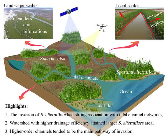
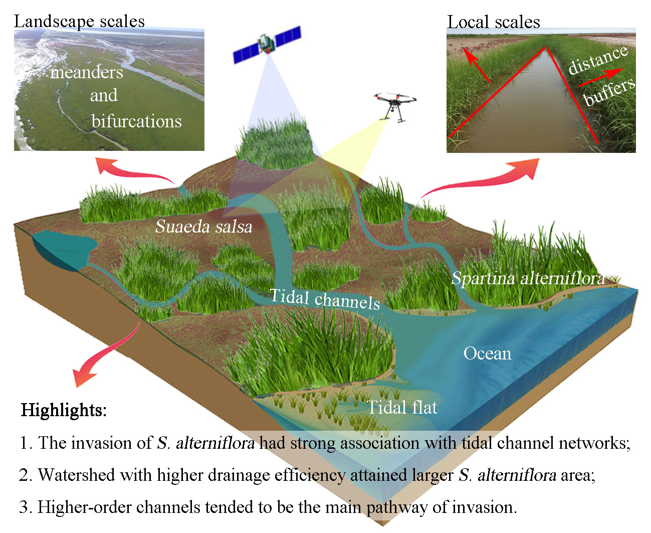
How Does Spartina alterniflora Invade in Salt Marsh in Relation to Tidal Channel Networks? Patterns and Processes

1
State Key Laboratory of Water Environment Simulation & School of Environment, Beijing Normal University, Beijing 100875, China
2
Yellow River Estuary Wetland Ecosystem Observation and Research Station, Ministry of Education, Dongying 257500, China
3
Tang Scholar, Beijing Normal University, Beijing 100875, China
*
Author to whom correspondence should be addressed.
These authors contributed equally to this work.
Remote Sens. 2020, 12(18), 2983; https://doi.org/10.3390/rs12182983
Submission received: 13 July 2020 / Revised: 9 September 2020 / Accepted: 10 September 2020 / Published: 14 September 2020
(This article belongs to the Section Biogeosciences Remote Sensing)

Abstract

:
Rapid invasion of Spartina alterniflora in coastal wetlands throughout the world has attracted much attention. Some field and imagery evidence has shown that the landward invasion of S. alterniflora follows the tidal channel networks as the main pathway. However, the specific patterns and processes of its invasion in salt marshes in relation to tidal channel networks are still unclear. Based on yearly satellite images from 2010 to 2018, we studied the patterning relationship between tidal channel networks and the invasion of S. alterniflora at the south bank of the Yellow River Estuary (SBYRE). At the landscape (watershed and cross-watershed) scale, we analyzed the correlation between proxies of tidal channel network drainage efficiency (unchanneled flow lengths (UFL), overmarsh path length (OPL), and tidal channels density (TCD)) and spatial distribution of S. alterniflora. At the local (channel) scale, we examined the area and number of patches of S. alterniflora in different distance buffer zones outward from the tidal channels. Our results showed that, overall, the invasion of S. alterniflora had a strong association with tidal channel networks. Watershed with higher drainage efficiency (smaller OPL) attained larger S. alterniflora area, and higher-order (third-order and above) channels tended to be the main pathway of S. alterniflora invasion. At the local scale, the total area of S. alterniflora in each distance buffer zones increased with distance within 15 m from the tidal channels, whereas the number of patches decreased with distance as expansion stabilized. Overall, the S. alterniflora area within 30 m from the tidal channels remained approximately 14% of its entire distribution throughout the invasion. The results implicated that early control of S. alterniflora invasion should pay close attention to higher-order tidal channels as the main pathway

Graphical Abstract

1. Introduction

Over the last decades, perennial rhizomatous Spartina alterniflora, as a dreaded invader spreading rapidly to estuaries and coastal salt marshes throughout the world, has received much attention [1,2,3]. In tidal saltmarshes, sexual reproduction by seeds and asexual propagation by tillering and rhizome production are the main ways for S. alterniflora to successfully colonize in new habitats [4,5,6]. The invasion of S. alterniflora is influenced by numerous biotic and abiotic factors, such as nutrients [7] and herbivores [8], as well as local geomorphology [9,10] and hydrology [11,12], which can be further linked to tidal channels as ubiquitous landscape configuration controlling tidal prism and inundation, fluxes of sediments, nutrients, and hydrochorous seed dispersal in and between salt marshes [13,14,15]. The latter can be of disproportionate importance by mediating colonization of remote habitats [16,17]. More recently, some field observations and aerial images in Chinese shorelines have shown that the landward invasion of S. alterniflora follows the tidal channel networks as the main pathway [13,18,19]. Therefore, to make a robust prediction of S. alterniflora invasion for coastal wetland management, it is important to improve our understanding of the role of tidal channel networks in its invasion in coastal salt marshes.
The previous studies focused on the influence of tidal channels on the distribution of salt marsh plants have demonstrated that both native and invasive species tended to colonize along the tidal channels [9,20,21]. Some studies have also reported that salt marsh plants showed a significant increase in abundance along channel banks, which was followed by a decrease with lateral distance further away from the tidal channels [22,23]. This may be attributed to the lower salinity [24], higher moisture [25], higher nutrient level [10], and better-aerated condition [26] near tidal channels. Some morphological features of tidal channels (e.g., bifurcations and meanders) are fundamental in determining species distribution patterns in salt marsh, and marshes with highly sinuous channels were found to possess more productive vegetation [27]. Moreover, small and shallow tidal channels tended to retain more nutrients and particulates within the salt marsh [10,23], for which a mathematical function was proposed by Sanderson et al. [28] to measure the “channel influence” at each point of the adjacent area as a function of its distance to channels as well as channel order.
Some studies have examined the interplay between exotic species invasion and tidal channel networks. Amongst them, Hou et al. [29] analyzed the qualitative relationship between the size and alignment of tidal channels and the invasion area and rate of S. alterniflora, and found that S. alterniflora mainly invaded landward along the main tidal channels aligned in the land–sea direction. Schwarz et al. [13] studied the impact of altered bio-geomorphic feedbacks caused by S. alterniflora invasion on tidal channel networks through proxies such as unchanneled flow lengths (UFL) and overmarsh path length (OPL) as indicators of tidal channel drainage efficiency [30,31], and found that the tidal channel drainage efficiency in the invaded site had a decreasing tendency throughout S. alterniflora invasion. Tidal channels density (TCD) is another proxy commonly used to define the drainage efficiency of a tidal channel network based on channelized length [31]. The conventional TCD was defined as a single integral parameter out of the entire channel network, and did not take into account the spatial heterogeneity of channel order and sinuosity that are of great importance to drainage efficiency of a tidal channel network in salt marshes [10,23]. Considering this limitation, Zheng et al. [21] proposed a modified TCD as a spatially variable index, and observed a significant negative correlation between modified TCD and fractional vegetation cover (FVC) at landscape scales in a S. alterniflora invaded salt marsh.
By far, the majority of the previous studies [10,20,23] have focused on the response of salt marsh plants to the abiotic factors (e.g., salinity, inundation, and elevation) near tidal channels at local scales, typically through field surveys with limited sampling plots or transects. A few studies [9,21,23] have attempted to clarify the spatial relationship between salt marsh vegetation distribution patterns and tidal channels at landscape scales using aerial images, but the specific patterns and processes of exotic species invasion in salt marshes in relation to tidal channel networks still remain elusive. On an analogous note, linear wetlands such as channels, ditches, or roadsides as highly connected networks have been recognized as serving corridors facilitating species invasion at the landscape scale [32].
In this study, we explore the effects of tidal channel networks on the spatiotemporal invasion dynamics and distribution patterns of S. alterniflora at both local and landscape scales at a typical coastal salt marsh at the Yellow River Estuary (YRE), China. This salt marsh has experienced fast areal expansion of S. alterniflora since 2013 [33], and the intertidal zone is free of intensive human disturbances, allowing us to observe the invasion and distribution patterns of S. alterniflora under close to natural conditions. In this paper, we aim to: (1) investigate the spatiotemporal dynamics of S. alterniflora invasion at both local and landscape scales; and (2) quantify the patterns and processes of the invasion with respect to the tidal channel networks. The ultimate goal is to provide references to improve the understanding of S. alterniflora invasion and its control for coastal wetland management.

2. Materials and Methods
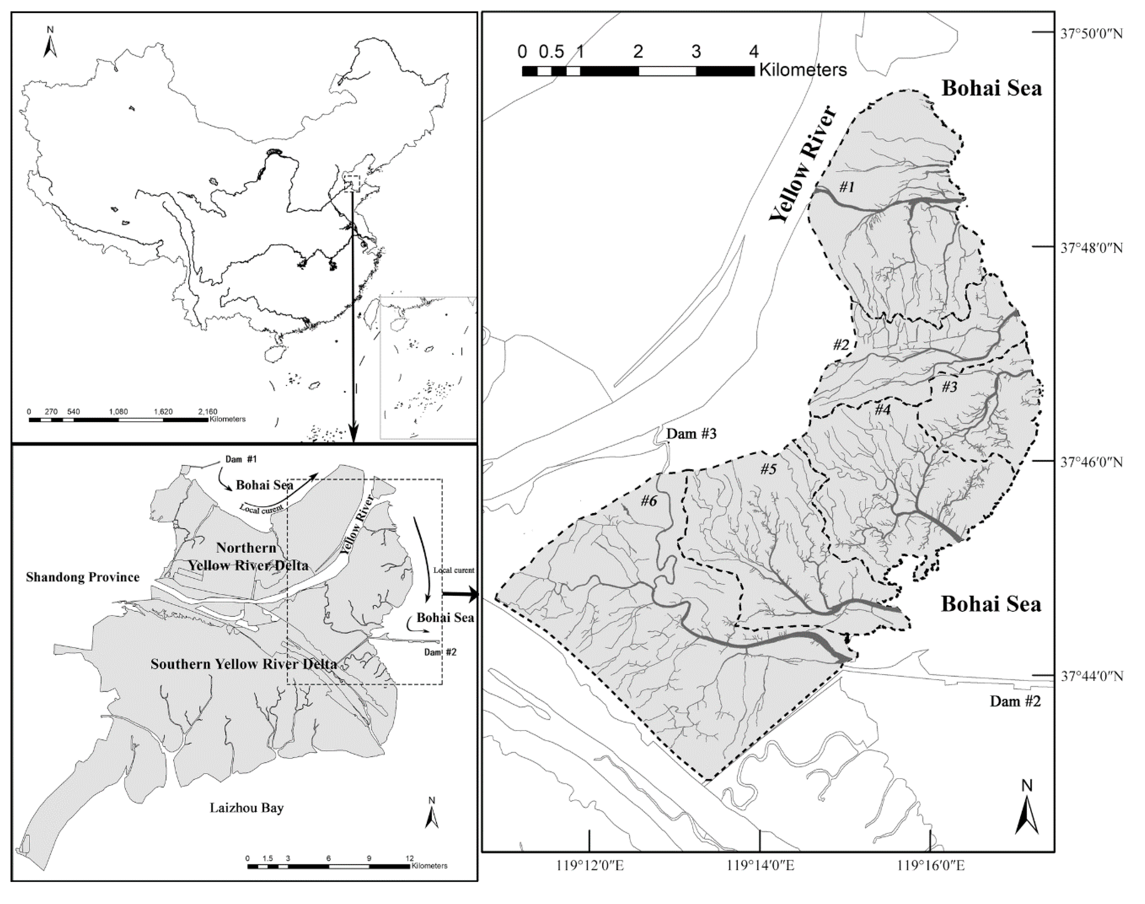
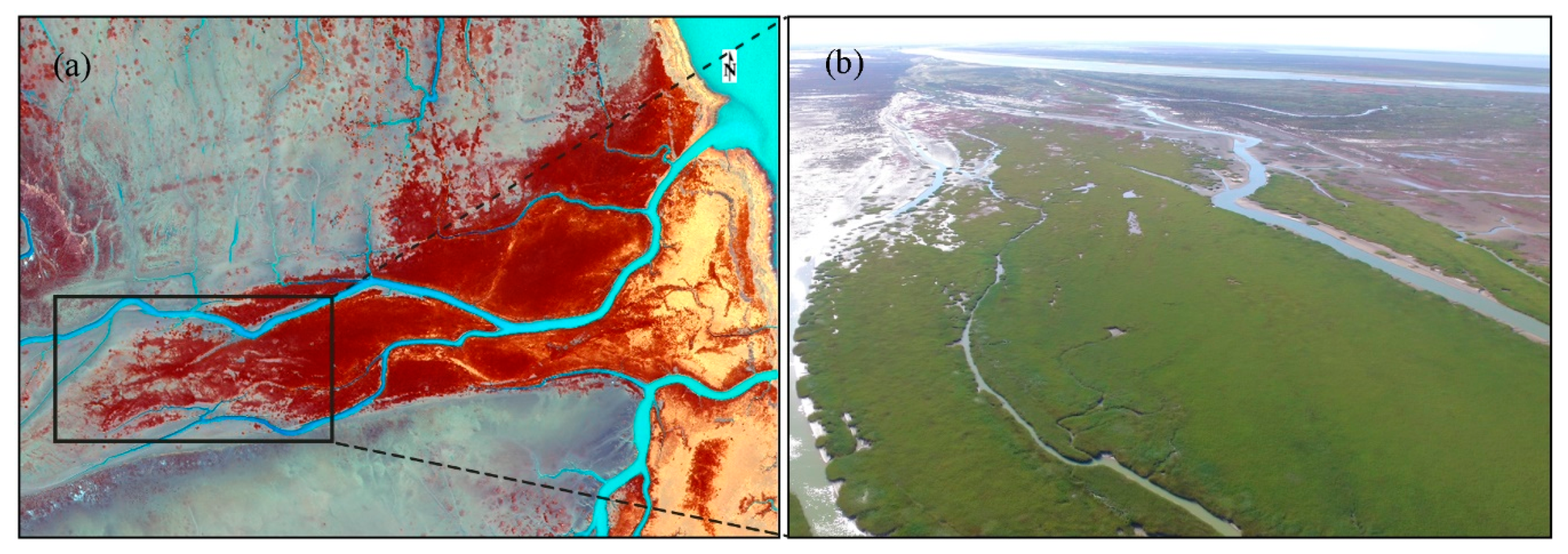
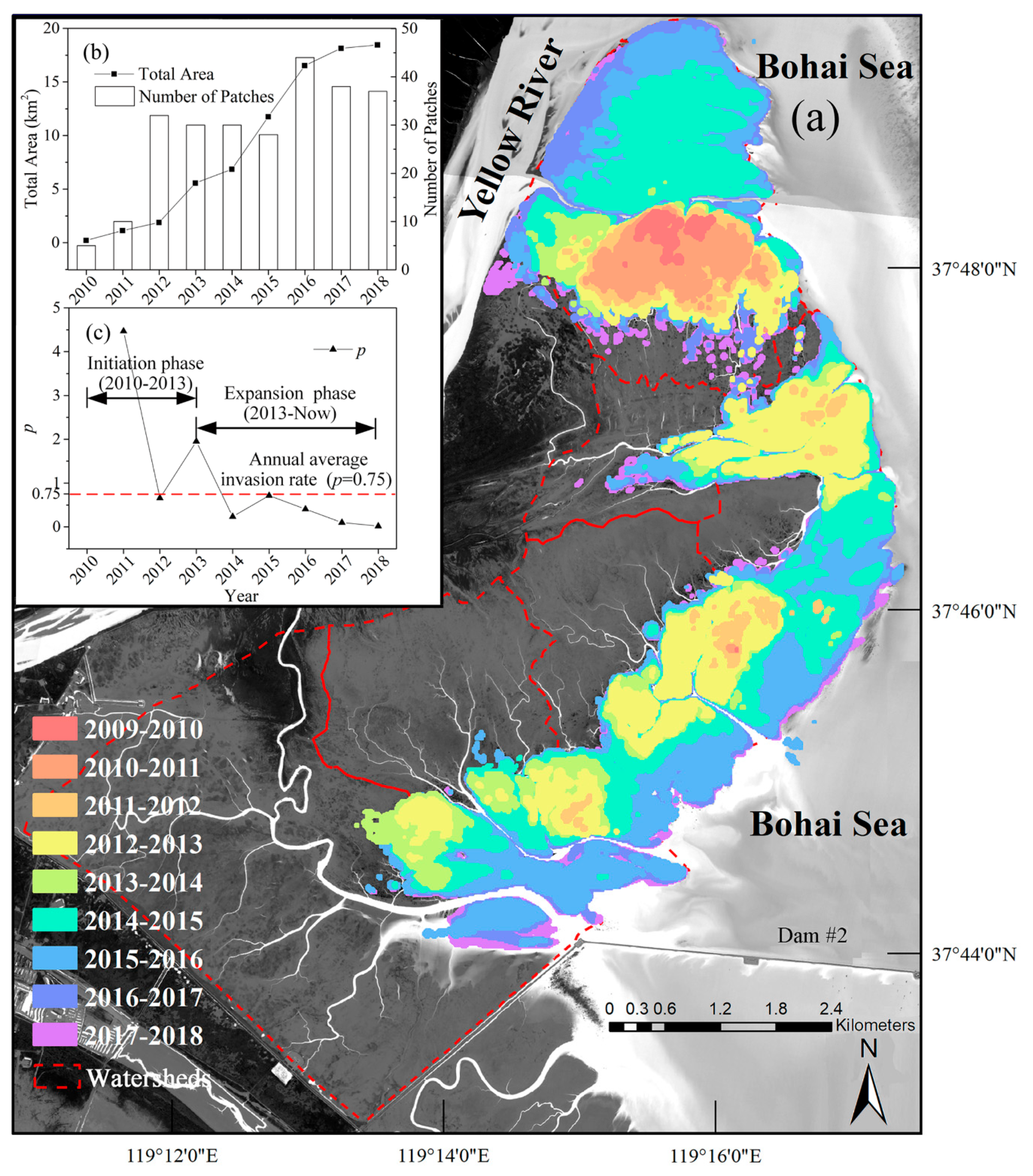
2.1. Study Area

We conducted the research at the YRE located in Dongying City, Shandong Province, China (118°68′E–119°34′E; 37°77′N–38°12′N) (Figure 1). The study area is characterized by a semi-humid continental monsoon climate with four distinctive seasons (Jiang et al., 2013). The annual mean temperature is 11.5 to 12.4 °C, and the annual mean precipitation ranges from 576.7 to 596.9 mm [34,35]. The relative elevation to sea level (Yellow Sea Datum, YSD) ranges from −0.7 to 0.63 m [36]. Previously, Suaeda salsa, Tamarix chinensis, and Phragmites australis were the dominant native species in the coastal salt marshes [33].
S. alterniflora is a perennial rhizomatous grass native to the Gulf and Atlantic coasts of North America. It was originally introduced to East China in 1979 for beach protection and enhancing sedimentation, and nowadays has aggressively invaded a wide expanse of Chinese shoreline [37,38]. As such, S. alterniflora was listed as one of the 16 invasive species by the Environmental Protection Bureau of China in 2003. S. alterniflora was purposely introduced to the tidal flats of Wuhaozhuang to the north of Gudong oil field at the YRE in 1990, and had occupied the low marshes and spread out to the high marshes since 2013 [33,39,40]. In recent years, some field and imagery evidence has been reported that the invasion of S. alterniflora followed the tidal channel networks as the main pathways [13,18,19]. At the YRE, we have observed the same phenomenon from remote sensing images (Figure 2a) and field surveys (Figure 2b).
The study area is located at a well-developed tidal channel system at the South Bank of the Yellow River Estuary (SBYRE), which contains 6 watersheds (Figure 1). Due to the favorable hydrodynamic conditions with relatively weak waves and strong tidal currents, well-developed dendritic tidal channel networks formed at the SBYRE [41]. As a result, S. alterniflora seeds can be dispersed along the tide channel networks throughout salt marshes, which also partly contributed to the rapidly expanding S. alterniflora communities in this area [39].
Due to the bidirectional flow in the tidal channels, the terrestrial approach of delineating watersheds based on the elevation data proved inapplicable in intertidal systems [31]. Following previous studies [30,42], we delineated the watershed areas of our study area using the principle proposed by Marani et al. [31], i.e., the divide between watersheds is approximately equidistant from adjacent tidal channels. Therefore, the seaward boundary was determined by the inlet of the tidal channel network, and the lateral boundary was delineated with equal distances to tidal channels in adjacent watersheds.

2.2. Data Acquisition and Preprocessing

Given that S. alterniflora first colonized the study area in 2010, salt marsh tidal channel networks and land cover data from 2010 to 2018 were acquired from yearly satellite images (Table 1) in this study. Amongst them, cloud-free Landsat images were mainly used to extract the distribution of S. alterniflora and study its invasion patterns at landscape scale, whereas the high-resolution GaoFen images with cloud cover less than 1% were used to extract both S. alterniflora and tidal channel networks and study their relationship at local scales. Landsat images were downloaded from the United States Geological Survey (https://earthexplorer.usgs.gov/), including a panchromatic band of 15 m resolution and multi-spectral bands of 30 m resolution. All Landsat images were selected at low tides in winter to facilitate distinguishing S. alterniflora from other annual species. GaoFen images were downloaded from the China Centre for Resources Satellite Data and Application (http://www.cresda.com/CN/), including a panchromatic band and four multi-spectral bands (near-infrared, red, green, and blue). Given its long revisit period and high cloud cover during the study period, the selection of the GaoFen images was not able to match the seasons and tidal levels of the selected Landsat images.
Ground surveys were conducted in October 2018, and a series of aerial images were acquired by drone while sampling. Overall, a total of 145 verification samples containing 43 points of S. alterniflora and 102 points of non-S. alterniflora were collected. The location of sampling sites is shown in Figure S3 in Supplementary Material.
Using ENVI 5.3 software, all images were processed for radiometric calibration and FLAASH atmospheric correction. To improve image resolution, the panchromatic band was merged with multispectral bands through Gram–Schmidt pan sharpening in the toolbox. Afterwards, all images were projected to the Universal Transverse Mercator (UTM) coordinate system, Zone 50 North. To reduce the potential position errors with GaoFen images, we made geometric corrections based on ground control points (GCPs) using the Landsat image as a reference in ArcGIS10.2. To standardize the image dataset and retain the spatial details, all Landsat and GaoFen images were resampled to a pixel size of 15 m × 15 m and 2 m × 2 m, respectively. Before we performed the image segmentation, all images were clipped using the boundary of the study area.

2.3. Classification Methods and Accuracy Assessment

Following Vandenbruwaene et al. [42] and Zheng et al. [21], normalized difference water index (NDWI) was adopted alongside visual interpretation to identify the tidal channels in ENVI 5.3. After interpretation, channel orders were determined using the method of Strahler [43]. Based on the S. alterniflora growth characteristics and some previous interpretation methods [38,44,45], maximum likelihood classifier was adopted to interpret vegetation in the salt marsh in ENVI 5.3. S. alterniflora and non-S. alterniflora patches were identified and refined by visual interpretation. There are distinct interspecific differences between S. alterniflora and the other species in the images in winter: Mid-low intertidal zones near the sea are often occupied with S. alterniflora, while Suaeda salsa would grow in the lower moisture areas far from the sea [46]; Phragmites australis is mainly distributed along the banks of the Yellow River, and a relatively clear boundary is visible to separate P. australis from S. alterniflora [47]; Zostera japonica, a seagrass mostly distributed seaward from S. alterniflora patches, dies off each year after September [48]. Since newly colonized patches of S. alterniflora are small in size and difficult to discern, to minimize biasing dispersal data with classification errors, uncertain patches of S. alterniflora were refined by contrasting the context features on at least two years of images to determine the final land cover types. Specifically, we took the previous classification results as a thematic layer to segment the next image until all images were classified. Results of the remote sensing image interpretation were digitized into binary raster images with 1 for S. alterniflora, and 0 otherwise.
A total of 145 field survey samples were recorded by a series of aerial images acquired by drone in 2018. For other years lacking field survey data, 100 independent random sampling points were generated each year in the study area in Arcgis10.2 to verify the classification results of 2010–2017 [49]. These random points were classified into S. alterniflora and non-S. alterniflora by referring to relevant literature [47] and consulting with local experts and experienced interpreters. In this study, we randomly collected 50% of the ground truth points as training samples, and the others as validation samples. Confusion matrices were created for each year, and the overall accuracy, user accuracy, producer accuracy, and Kappa coefficient were calculated to measure the agreement between our classification results and the validation points [38,49,50].

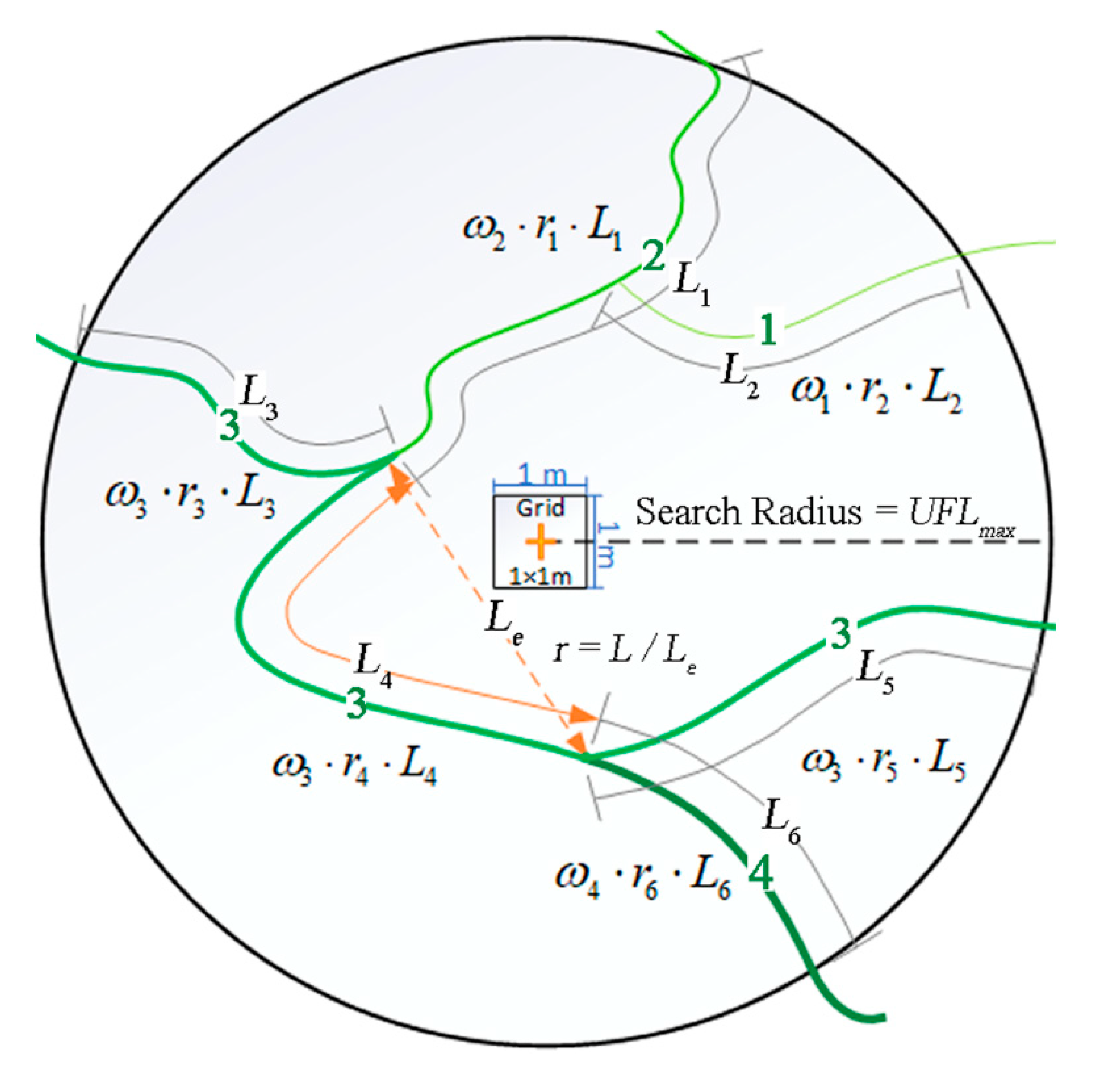
2.4. Quantifying Tidal Channel Properties

Drainage efficiency is commonly used to evaluate the spatial distribution of tidal channel networks in tidal flats [30,31,51]. Unchanneled flow lengths (UFL), overmarsh path length (OPL), and tidal channels density (TCD) are proxies that represent the drainage efficiency of tidal channel networks in individual watersheds in draining the site during the ebb and in distributing water and sediment during the flood tide [30]. Specifically, UFL is the hillslope distance of all pixels to the tidal channel network [27,51,52], representing the distance a water drop has to travel until it reaches the closest channel [21,30]. Because of the low elevation gradient in intertidal wetlands, Euclidean distance was generally used instead of slope distance to reduce computational cost [30,42]. Based on the semi-logarithmic exceedance probability distribution curve of the UFL, the negative reciprocal of the slope of the linear part by fitting a linear function can be calculated and termed as OPL. It represents the average distance that needs to be crossed within a marsh before encountering a tidal channel [31,42]. Therefore, smaller OPL means a well-distributed tidal channel network and hence higher drainage efficiency [30,31]. In this study, OPL was calculated separately for the 6 individual watersheds.
TCD is another commonly used metric that represents the drainage efficiency of tidal channel networks as the ratio of total channel length versus catchment area [30,31]. To make it a spatially variable index, Zheng et al. [21] redefined it on the basis of unit area. Previous studies have shown that network drainage efficiency is also affected by channel branching and meandering, and marshes with higher-order and highly sinuous channels possess relatively high efficiencies [27,28]. Therefore, we refine the spatially-varying TCD by incorporating a weighting factor related to the order and sinuosity of tidal channels. Figure 3 shows a grid cell with its circular neighborhoods. The refined TCD (TCDor) is calculated as follows:
T C D o r = i = 1 n ( ω o r d e r r i L i ) / A ,
where ωorder represents the channel order weighting factor; Li represents the length of the portion of the ith tidal channel that falls within the circle; ri represents the mean sinuosity ratio of ith tidal channel, which is defined as the ratio of the length of the tidal channel Li to the Euclidean distance between the starting and ending points; A represents the area of the search circle. The search radius is determined as 600 m by the maximum value of TCDor (TCDor, max) and its correlation coefficient with the distribution of S. alterniflora (see Text S1 in Supplementary Material for details). Sanderson et al. [28] developed the cumulative inverse squared distance function to measure the local “channel influence”, in which the weighting factor associated with channel order is dependent on channel cross-sectional area and maximum discharge. Following previous studies [28,41], the channel order weighting factors ωorder for 1st, 2nd, 3rd, 4th, and 5th -order channels are assigned as 0.1, 1, 10, 50, and 60, respectively.
In this paper, we calculated the OPL of each individual watershed to evaluate the overall drainage efficiency of tidal channel networks in the watershed. To further explore the relationship between tidal channel networks and S. alterniflora invasion, we calculated the spatially-varying UFL and TCD with different definitions in ArcGIS 10.2 using tidal channels extracted from GaoFen-2 image of the year 2018. Following Kearney and Fagherazzi [27], which showed that the statistics for the above third-order channels more accurately reflected the actual network structure, UFL was calculated on the above third-order tidal channels thereafter. Specifically, UFL1UFL6 are UFL corresponding to the #1–6 watershed, respectively; TCDo ( T C D o =   ( ω o r d e r L i ) / A ) was calculated only accounting for channel order; TCDr ( T C D r =   ( r i L i ) / A ) was calculated only accounting for channel sinuosity; TCDor was calculated accounting for both channel order and sinuosity as shown in Equation (1).

2.5. Quantifying the Invasion of S. alterniflora

Previous studies have shown that invasive plants like S. alterniflora usually undergo an exponential expansion [49]. The annual invasion rate was used to quantify the S. alterniflora invasion at the SBYRE [49]:
U a = U b × ( 1 + p ) N ,
where p represents the invasion rate; Ub and Ua are the area of S. alterniflora at the beginning and ending year of the period of interest, respectively; and N is the number of years.
Pearson correlation analyses were used to quantify the relationship between tidal channel networks and S. alterniflora in various watersheds at landscape scales. We further normalized the spatially-varying UFL and TCD metrics to the range of (0, 1) using their minimum and maximum values across the study area, and binned the normalized UFL and TCD metrics into ten equally-divided intervals and calculated the area proportion of S. alterniflora averaged over all pixels falling into each interval for each normalized metric (see Text S2 in Supplementary Material for details). The proportion of S. alterniflora was defined as the ratio of S. alterniflora pixels to the total amount of pixels within a working area.
To further characterize the spatiotemporal pattern of S. alterniflora invasion in relation to distance from tidal channel networks at the local scales, we examined the areas occupied by S. alterniflora from 2014 to 2018 using high-resolution GaoFen images, given that both the evolution of tidal channels and invasion rate of S. alterniflora gradually stabilized after 2014. Following Lathrop et al. [22], we examined the spatial distribution of S. alterniflora in relation to distance to the higher-order tidal channel at 5 m increments up to 30 m. Some common landscape indices were analyzed, such as the area proportion of S. alterniflora and number of patches at various distance buffer zones. These landscape metrics were calculated using Fragstats 4.2 [53].

3. Results

3.1. Spatiotemporal Dynamics of S. alterniflora Invasion and Tidal Channel Characteristics

The classification results are with an overall accuracy of 80–97% and a Kappa coefficient of 0.80–0.88, and the producer and user accuracies are greater than 0.80 (Table S1), which means that the S. alterniflora classification results are satisfactorily consistent with those obtained from the validation points. These accurate classification results were used for subsequent spatial analysis.
Figure 4a shows the S. alterniflora invasion process at the SBYRE from 2010 to 2018. Based on the change of the total area of S. alterniflora, we divided the invasion process into two phases, namely the initiation phase (2010–2013) and the expansion phase (2013–2018, Figure 4b,c) In 2010, S. alterniflora first colonized the spot near the YRE with a total area of 0.21 km2. During the initiation phase, although the total area and number of patches of S. alterniflora increased steadily, the annual invasion rate exhibited significant fluctuation (Figure 4b,c). After colonization and establishment near the YRE, it gradually spread southward along the coastline presumably driven by the nearshore currents, and subsequently expanded landward along the tidal channels. At the beginning of the expansion phase, invasion rate rebounded, which was followed by moderate fluctuation afterwards. While the total area of S. alterniflora kept increasing throughout the expansion phase, the number of S. alterniflora patches increased abruptly from the initiation to expansion phase and remained stable from 2013 to 2015. In 2016, both S. alterniflora area and number of patches increased dramatically and stabilized afterwards.
Table 2 documents the characteristics of the tidal channel networks in the various watersheds based on the GaoFen-2 image in 2018. The southernmost #6 watershed had the largest area and total channel length and yet the lowest drainage efficiency (largest OPL). The #4 watershed had the highest drainage efficiency of the tidal channel networks with the smallest OPL. During the initiation phase, while S. alterniflora areas increased immediately in the #1 and #4 watersheds, invasion of S. alterniflora in the remaining watersheds did not start until 2012. As the expansion phase kicked off in 2013, S. alterniflora areas in all watersheds gradually increased, albeit at different rates (Table 3). Invasion of S. alterniflora showed signs of slowing down in 2018 with an average total invasion rate of only 0.02, and the invasion rates of individual watersheds were all less than 0.01 except in the #6 watershed. As a newly colonized site, the #6 watershed still featured a substantial invasion rate of 0.16 in 2018, indicating the potential for further expansion in the subsequent years.
Presumably due to its location adjacent to the mouth of the Yellow River, which is among the most sediment-laden rivers in the world, #1 watershed experiences rapid progradation seaward. Therefore, we excluded the #1 watershed that is subject to potentially strong estuarine influence from the analysis, and found that the area of S. alterniflora in the remaining watersheds in 2018 showed a significant negative correlation with OPL, i.e., positive correlation with overall drainage efficiency of the watershed (Figure 5).

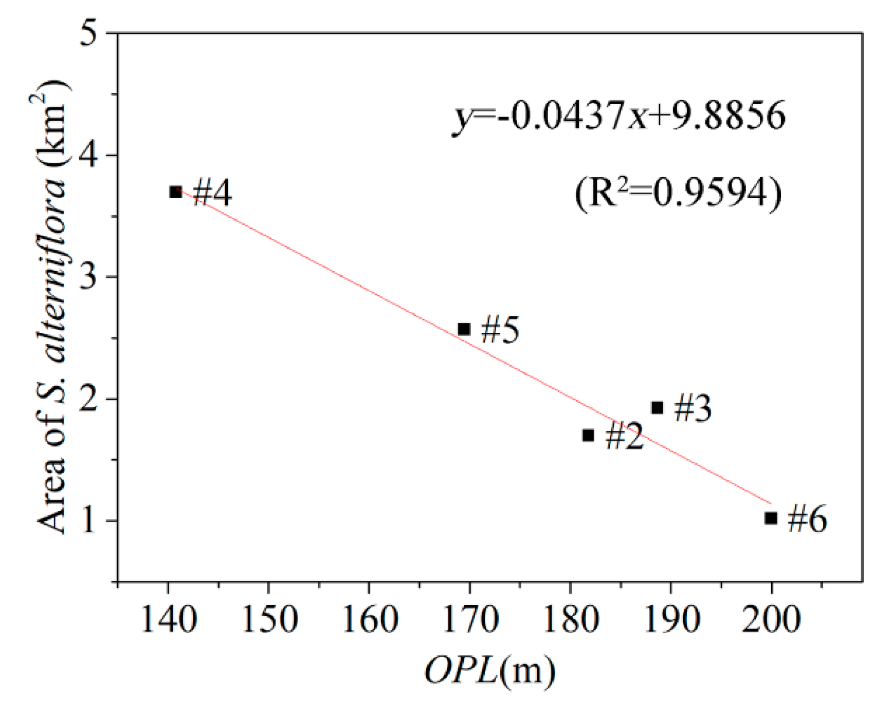
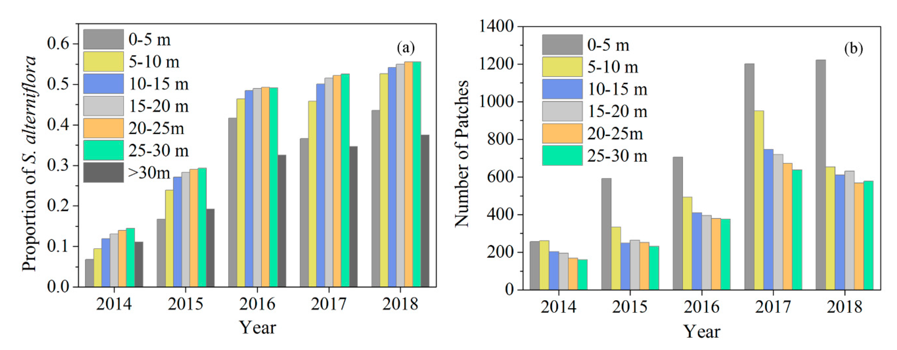
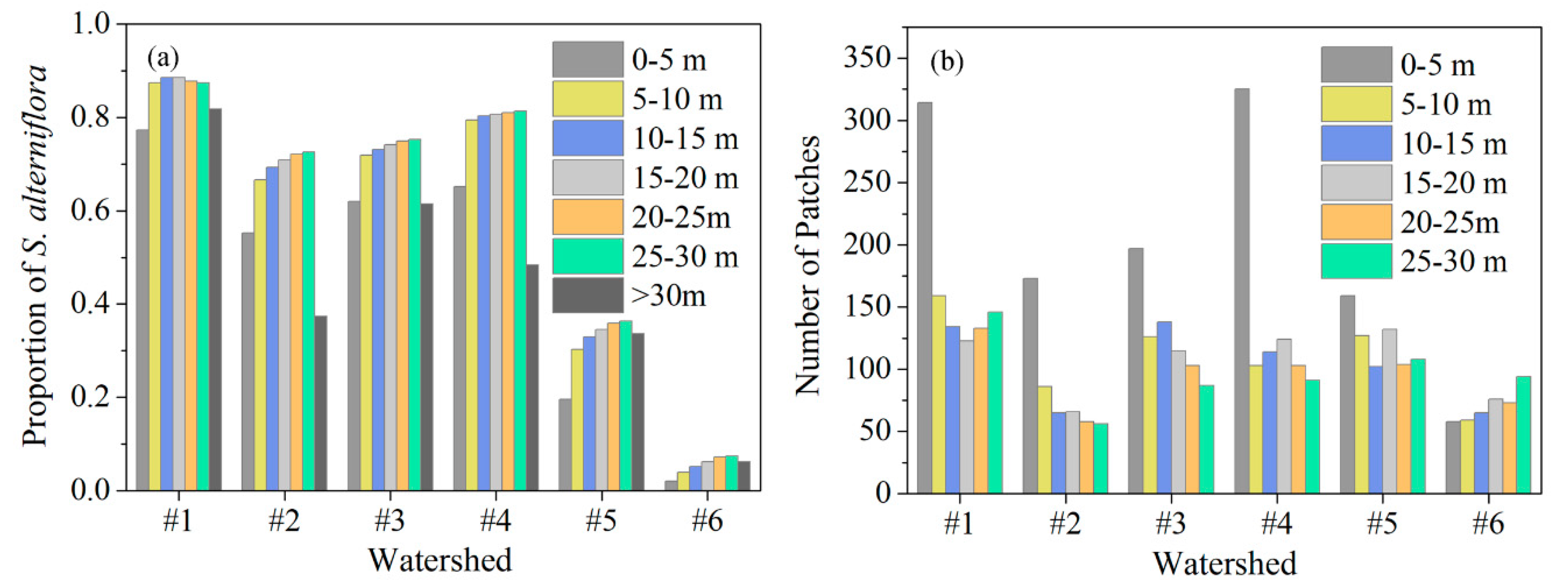
3.2. Relationship between Tidal Channels Networks and S. alterniflora Distribution at Landscape Scales

To further investigate the relationship between the morphology (e.g., bifurcations and meanders) of the tidal channel networks and the invasion of S. alterniflora at the landscape scale, we analyzed the distribution of S. alterniflora with respect to the spatially-varying drainage efficiency of tidal channel networks (UFL and TCD) (Figure 6). The area proportion of S. alterniflora with increasing drainage efficiency after normalization in the #1–6 watersheds are presented in Figure 7.
Figure 7 showed that there is a steady increase in the proportion of S. alterniflora with increasing TCDo until around 0.7, which suggested that different channel orders with different channel sizes had varying degrees of influence on the invasion pattern, and higher-order channels were more closely related to the distribution of S. alterniflora. On the contrary, no clear trend was observed between the area proportion of S. alterniflora and the TCDr. This is further verified by the curve of the TCDor being almost coincident with that of TCDo, which indicated that the influence of the channel curvature on the spatial distribution of S. alterniflora is relatively insignificant.
Furthermore, we analyzed the area proportion of S. alterniflora with increasing UFL. Results showed that with increasing UFL, the area proportion of S. alterniflora decreased steadily. This indicated that patches of S. alterniflora concentrated near the tidal channels, which became more sparse with increasing distance from the tidal channels, and could even vanish at sufficient distance. Similar trends were found in UFL2 through UFL6, amongst which S. alterniflora in the #4 watershed with the highest drainage efficiency exhibited the most prominent concentration toward the tidal channels, whereas the #6 watershed with the lowest drainage efficiency exhibited the least. By contrast, such trend could not be observed in the #1 watershed with significant estuarine influence. Notably, UFL1 reached a smaller maximum value of –0.6, which means the #1 watershed had relatively small UFL overall. Taking the above analysis together, it suggested that S. alterniflora tended to congregate at higher-order (third-order and above) channels, and the congregation became more prominent when the watershed is with a greater drainage efficiency.

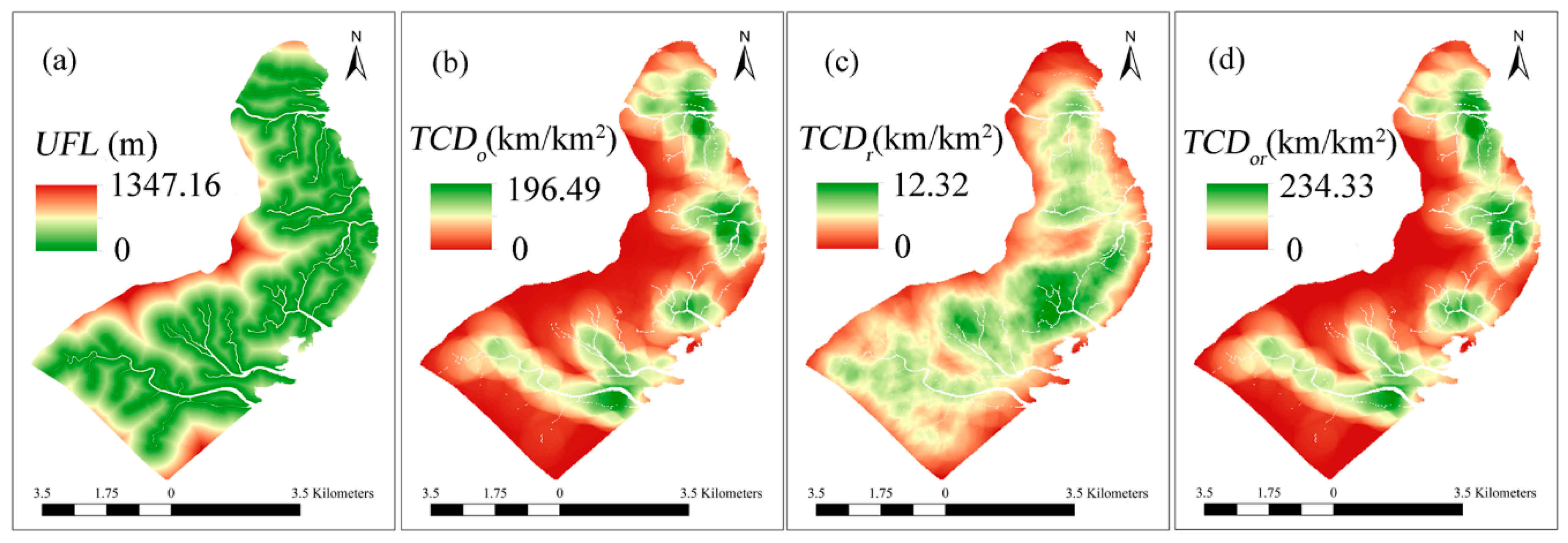
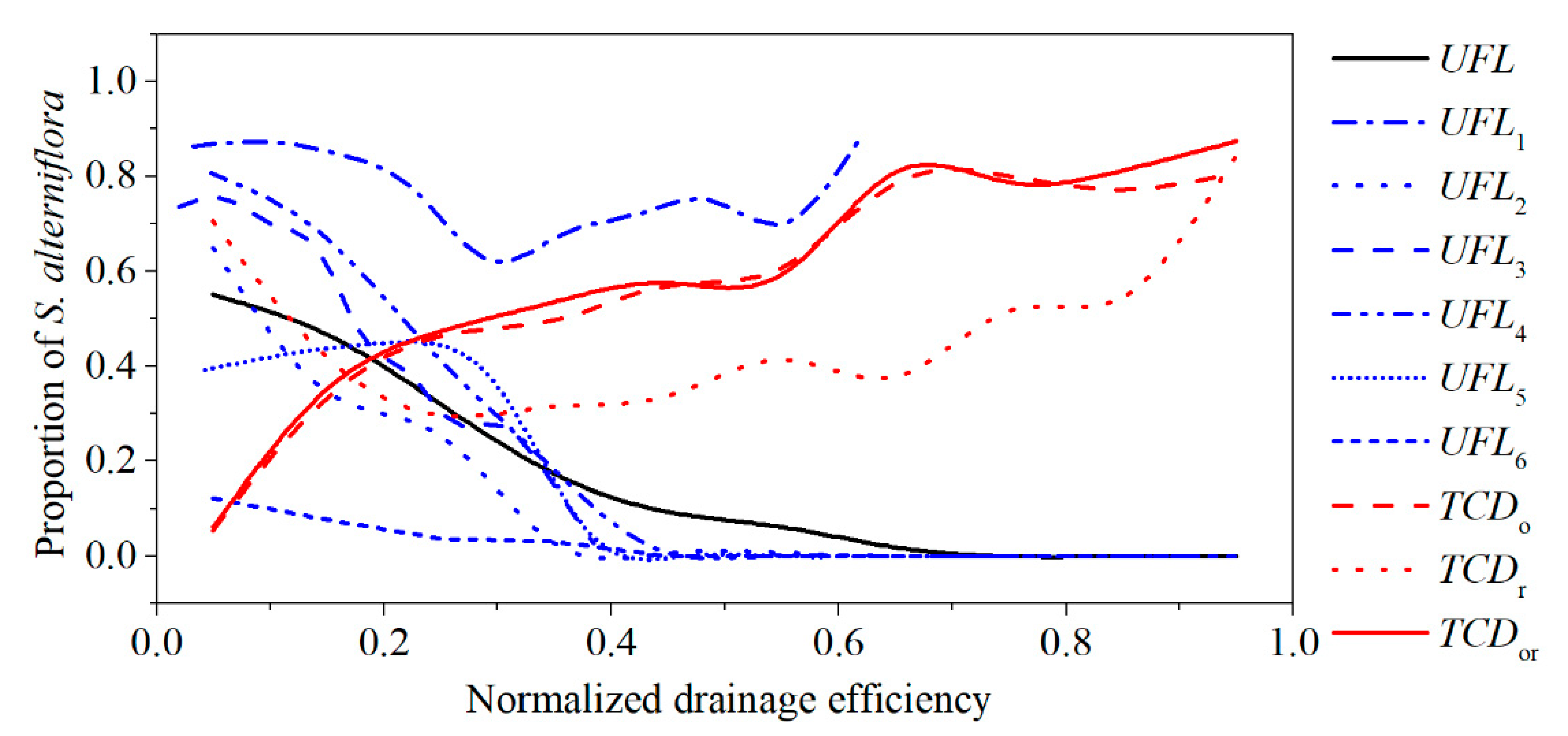
3.3. Relationship between Tidal Channel Networks and S. alterniflora Invasion at Local Scales

Figure 8 shows the variation of the S. alterniflora area and the number of patches within each distance buffer zone in 2014–2018. The overall increase and then stabilization of the area proportion of S. alterniflora, which represented the percentage areal distribution of the S. alterniflora along the distance gradient in Figure 8a, corroborates with the trend of variation illustrated in Figure 4b. After 2015, the number of S. alterniflora patches in the 0–5m distance buffer zone was significantly larger than in the other distance buffer zones (p < 0.01). However, the area proportion of S. alterniflora in the nearest zones were significantly smaller (p < 0.05). It increased with distance to tidal channels in the 0–15 m buffer zones, whereas no significant difference was observed in the 15–30 m buffer zones. Meanwhile, the area proportion of S. alterniflora beyond the 30 m buffer zones were relatively smaller during this period. Overall, the S. alterniflora area within 30 m from the tidal channel networks accounted for approximately 14% of the entire S. alterniflora area.
To further explore the relationship between tidal channel networks with different drainage efficiency and the spatial distribution of S. alterniflora, we performed the above analyses in each individual watershed in 2018 (Figure 9). Overall, the proportion of S. alterniflora within the 30 m buffer zones to the entire S. alterniflora area attained the largest value (nearly 20%) in the #2 watershed. This might be due to the better alignment of its higher-order tidal channels with the land-sea direction (i.e., east-west), which facilitates the tide-driven spreading along the tidal channels. The #6 watershed with the lowest drainage efficiency exhibited the lowest proportion (only 6%) of S. alterniflora distribution in the 0–30 m buffer zones. The invasion in the #6 watershed was presumably still in the initiation phase as reflected by both the proportion of S. alterniflora and number of S. alterniflora patches in buffer zone within 5 m smaller than in the outer zones. While in the #1–5 watersheds, the number of patches within 5 m buffer zones are significantly larger than the outer zones (p < 0.05), and the invasion of S. alterniflora seemed to have entered a relatively stable phase in 2018 (Table 3).

4. Discussion

During the past decades, the aggressive invasion and rapid expansion of S. alterniflora had threatened biodiversity and ecosystem functioning in coastal salt marshes along Chinese shorelines [18,54]. Some previous studies have shown that the landward invasion of S. alterniflora followed the tidal channel networks [13,19]. In this study, our results showed that the invasion of S. alterniflora had a strong association with tidal channel networks at both local and landscape scales, and the invasion patterns of S. alterniflora in different phases at different scales exhibited some different characteristics.
Tidal channel networks are ubiquitous features of salt marsh ecosystems, playing a crucial role by controlling hydrodynamics, fluxes of sediments, nutrients, and biota in and between salt marshes [13,23,55]. Maheu-Giroux and de Blois [32] demonstrated that linear wetlands such as channels, ditches, or roadsides could serve as corridors facilitating invasion at the landscape scale because of their spatial configuration as highly connected networks. Our results showed that tidal channel networks acted as corridors in the intertidal salt marsh, leading to the rapid landward invasion of S. alterniflora along the tidal channels in the expansion phase (Figure 4). Our results further revealed that the invasion of S. alterniflora in the watershed with higher drainage efficiency was more expansive (Figure 5) and exhibited more concentrated spreading along tidal channel networks (Figure 7), which highlights the importance of the tidal channel network in the S. alterniflora invasion.
At the landscape scale, tidal channel morphology, such as bifurcations and meanders, has great influence on the distribution of S. alterniflora. Sanderson et al. [23] reported from the field survey that the vegetation showed significant increase in abundance approximately linearly with channel size, which was roughly correlated with channel order. The results of spatial analysis between UFL and the area proportion of S. alterniflora showed that the above third-order tidal channels played more important roles in the distribution of S. alterniflora (Figure 7), which is consistent with the finding of Hou et al. [29] and Kearney and Fagherazzi [27]. Furthermore, a steady increase was found in the area proportion of S. alterniflora with increasing TCDo, reaffirming that the effects of tidal channels on the invasion and distribution of S. alterniflora strongly depended on their channel orders.
The distribution of S. alterniflora in the early and late expansion phase near the tidal channels at the local scales alongside the gradient of the various relevant physical factors. Tidal channels are prominent salt marsh agents that can provide spatially differential physical constraints (e.g., elevation, inundation, salinity etc.) on plants growth with a gradient perpendicular to the channels [10,56,57]. Generally, a tidal channel shapes sequential geomorphic features such as marginal bank (0–5 m), transition (5–15 m), and marsh interior (>15 m) [58]. Each of these geomorphic features receives varying degrees of influence from the tidal channels, which eventually contributes to the local scale distribution pattern associated with distance from the tidal channels [14,22,23]. According to Kim et al. [10], the marginal bank zone is the lowest in elevation, which contributes to its frequent inundation and lower salinity. Elevation in the transition zone becomes higher with increasing lateral distance from the channel bank, and the marsh interior zone is mid-high with infrequent inundation and highest salinity.
From our local-scale analysis, the area proportion of S. alterniflora in the buffer zone within 5 m was significantly smaller than in the other distance buffer zones in the late expansion phase after 2015 (Figure 8a), which was consistent with expansion patterns of Phragmites australis in Piermont Marsh, New York [22]. The area proportion of S. alterniflora increased significantly with the distance to tidal channels in the 0–15 m buffer zones (Figure 8a). This may be due to lower elevation and increasing inundation in distance buffer zones near tidal channels [11,21]. However, there was no significant difference of S. alterniflora distribution in the 15–30 m buffer zones. Sanderson et al. [23] drew a similar conclusion that, depending on the distance from the tidal channels, the tidal channels had influence on the vegetation to varying degrees, especially within a 20 m distance range. Besides, Howes and Goehringer [59] also showed that tidal drainage can influence hydrology up to 15 m from tidal channel banks, consistent with the different trend starting from 15 m observed in our study.
Our research established that the invasion of S. alterniflora had strong association with tidal channel networks, and higher-order channels tended to be the main pathway of invasion. Various mechanisms behind the manifested pattern have been examined in the literature. For instance, as the main driving force for the colonization of S. alterniflora in new habitats [60], tidal flow controls the dispersal of the seeds in and between saltmarshes [61], thus affecting the spatiotemporal development of saltmarsh vegetation. While tidal channels, as ubiquitous landscape configuration controlling tidal prism and inundation, provide a important pathway for seed dispersal [15], which directly affects the distance, strength, and effectiveness of plant expansion. In addition to surface effects, Howes and Goehringer [59] illustrate that much of the drainage is belowground, which may also impact the survivorship of the plants as it increases advection of nutrients and sulfides.

5. Conclusions

Our quantitative analysis based on remote sensing images proved that the invasion of S. alterniflora had a strong association with tidal channel networks. S. alterniflora showed a preference to colonize near the tidal channels, leading to rapid landward invasion in its expansion phase. At the landscape scale, the invasion of S. alterniflora in salt marsh with higher drainage efficiency of tidal channel networks (smaller OPL) attained larger S. alterniflora area and showed more concentrated spreading along tidal channels. Besides, tidal channel orders exhibited great influence on channel effects on S. alterniflora, and the higher-order (above third-order) tidal channels tended to play the dominant roles in the invasion and distribution of S. alterniflora, whereas the effects of smaller channels were insignificant. At local scales, the distance from tidal channels had great influence on the vegetation distribution, especially within 15 m to the tidal channels. While area proportion of S. alterniflora increased with distance within 15 m from the tidal channels, the number of patches decreased with distance as expansion stabilized. Overall, the S. alterniflora area within 30 m from the tidal channels remained approximately 14% of the entire distribution throughout the invasion.
Following Chirol et al. [30] who recommended OPL as a valid proxy of tidal channel networks drainage efficiency, this paper advocates its utility as an indicator of overall watershed-level drainage efficiency, whereas applicability of spatially-varying UFL and TCD was also demonstrated such that local nuances of the tidal channel networks such as tidal channel order and sinuosity can be effectively incorporated as well. While our results suggested watershed with more efficient channel networks are prone to larger scale S. alterniflora invasion, Schwarz et al. [13] found that the tidal channel drainage efficiency in the invaded site decreased following S. alterniflora invasion, potentially leading to a negative feedback. This needs to be checked in the future as an important mechanism of S. alterniflora invasion in relation to tidal channel networks.
To the best of our knowledge, this is the first quantitative study to correlate the patterns of tidal channel networks with plant invasion dynamics at both local and landscape scales, which can provide references to improve the understanding of S. alterniflora invasion and its control for coastal wetland management. Our research suggested that the invasion control of S. alterniflora could attempt to control seed dispersal along the tidal channels, especially in the higher-order channels that tended to play a more dominant role.

Supplementary Materials

The following are available online at https://www.mdpi.com/2072-4292/12/18/2983/s1, Text S1: The method for determining the optimal search radius for the refined Tidal Channels Density (TCD), Text S2: The method for analyzing the correlation between proxies of tidal channel network drainage efficiency (Unchanneled Flow Lengths (UFL) and Tidal channels density (TCD)) and spatial distribution of S. alterniflora, Figure S1: Variation of the maximum value of TCDor (TCDor, max) and its correlation coefficient with the distribution of S. alterniflora as a function of search radius, Figure S2: Division of S. alterniflora pixels based on normalized drainage efficiency, Figure S3: Location of sampling sites, Table S1: Confusion matrix of S. alterniflora classification result from 2010 to 2018.

Author Contributions

Conceptualization, L.S., D.S. and B.C.; Methodology, L.S., T.X. and X.M.; Validation, D.S., W.G. and T.X.; Investigation, L.S., X.M. and Z.N.; Data Curation, L.S.; Writing—Original Draft Preparation, L.S.; Writing—Review & Editing, D.S.; Supervision, D.S. and B.C.; Funding Acquisition, B.C. All authors have read and agreed to the published version of the manuscript.

Funding

This research was funded by the Key Project of National Natural Science Foundation of China (Grant No. 51639001), the Joint Funds of the National Natural Science Foundation of China (Grant No. U1806217), and the Interdisciplinary Research Funds of Beijing Normal University.

Acknowledgments

We thank the Yellow River Delta National Nature Reserve for its long-term support of our ecological research programs.

Conflicts of Interest

The authors declare there are no conflict of interest.

References

  1. Strong, D.R.; Ayres, D.R. Ecological and evolutionary misadventures of spartina. Ann. Rev. Ecol. Evol. Syst. 2013, 44, 389–410. [Google Scholar] [CrossRef]
  2. Zheng, S.; Shao, D.; Sun, T. Productivity of invasive saltmarsh plant Spartina alterniflora along the coast of China: A meta-analysis. Ecol. Eng. 2018, 117, 104–110. [Google Scholar] [CrossRef]
  3. Ning, Z.; Xie, T.; Liu, Z.; Bai, J.; Cui, B. Native herbivores enhance the resistance of an anthropogenically disturbed salt marsh to Spartina alterniflora invasion. Ecosphere 2019, 10, e02565. [Google Scholar] [CrossRef] [Green Version]
  4. Daehler, C.C.; Strong, D.R. Status, prediction and prevention of introduced cordgrass Spartina spp. invasions in Pacific estuaries, USA. Biol. Conserv. 1996, 78, 51–58. [Google Scholar] [CrossRef]
  5. Xiao, D.; Zhang, L.; Zhu, Z. The range expansion patterns of Spartina alterniflora on salt marshes in the Yangtze Estuary, China. Estuar. Coast. Shelf Sci. 2010, 88, 99–104. [Google Scholar] [CrossRef]
  6. Davis, H.G.; Taylor, C.M.; Civille, J.C.; Strong, D.R. An Allee effect at the front of a plant invasion: Spartina in a Pacific estuary. J. Ecol. 2004, 321–327. [Google Scholar] [CrossRef]
  7. Tyler, A.C.; Lambrinos, J.G.; Grosholz, E.D. Nitrogen inputs promote the spread of an invasive marsh grass. Ecol. Appl. 2007, 17, 1886–1898. [Google Scholar] [CrossRef]
  8. Grosholz, E. Avoidance by grazers facilitates spread of an invasive hybrid plant. Ecol. Lett. 2010, 13, 145–153. [Google Scholar] [CrossRef]
  9. Marani, M.; Silverstri, S.; Belluco, E.; Camuffo, M.; D’Alpaos, A.; Lanzoni, S.; Marani, A.; Rinaldo, A. Patterns in tidal environments: Salt-marsh channel networks and vegetation. in IGARSS. In Proceedings of the IEEE International Geoscience and Remote Sensing Symposium (IEEE Cat. No. 03CH37477), Toulouse, France, 21–25 July 2003. [Google Scholar]
  10. Kim, D.; Cairns, D.M.; Bartholdy, J. Tidal creek morphology and sediment type influence spatial trends in salt marsh vegetation. Prof. Geogr. 2013, 65, 544–560. [Google Scholar] [CrossRef]
  11. Zhu, X.; Meng, L.; Zhang, Y.; Weng, Q.; Morris, J. Tidal and meteorological influences on the growth of invasive spartina alterniflora: Evidence from UAV remote sensing. Remote Sens. 2019, 11, 1208. [Google Scholar] [CrossRef] [Green Version]
  12. Li, R.; Yu, Q.; Wang, Y.; Wang, Z.B.; Gao, S.; Flemming, B. The relationship between inundation duration and Spartina alterniflora growth along the Jiangsu coast, China. Estuar. Coast. Shelf Sci. 2018, 213, 305–313. [Google Scholar] [CrossRef]
  13. Schwarz, C.; Ysebaert, T.; Vandenbruwaene, W.; Temmerman, S.; Zhang, L.; Herman, P.M.J. On the potential of plant species invasion influencing bio-geomorphologic landscape formation in salt marshes. Earth Surf. Process. Landf. 2016, 41, 2047–2057. [Google Scholar] [CrossRef]
  14. Tyler, A.C.; Zieman, J.C. Patterns of development in the creekbank region of a barrier island Spartina alterniflora marsh. Mar. Ecol. Prog. Ser. 1999, 180, 161–177. [Google Scholar] [CrossRef] [Green Version]
  15. Shi, W.; Shao, D.; Gualtieri, C.; Purnama, A.; Cui, B. Modelling long-distance floating seed dispersal in salt marsh tidal channels. Ecohydrology 2020, 13, e2157. [Google Scholar] [CrossRef]
  16. Shimamura, R.; Kachi, N.; Kudoh, H.; Whigham, D.F. Hydrochory as a determinant of genetic distribution of seeds within Hibiscus moscheutos (Malvaceae) populations. Am. J. Bot. 2007, 94, 1137–1145. [Google Scholar] [CrossRef] [Green Version]
  17. Van der Stocken, T.; Vanschoenwinkel, B.; de Ryck, D.J.; Bouma, T.J.; Dahdouh-Guebas, F.; Koedam, N. Interaction between water and wind as a driver of passive dispersal in mangroves. PLoS ONE 2015, 10, e0121593. [Google Scholar] [CrossRef] [Green Version]
  18. Qi, M.; Sun, T.; Zhang, H.; Zhu, M.; Yang, W.; Shao, D.; Voinov, A. Maintenance of salt barrens inhibited landward invasion of Spartina species in salt marshes. Ecosphere 2017, 8, e01982. [Google Scholar] [CrossRef]
  19. Wang, J.; Liu, H.; Li, Y.; Liu, L.; Xie, F. Recognition of spatial expansion patterns of invasive Spartina alterniflora and simulation of the resulting landscape-changes. Acta Ecol. Sin. 2018, 38, 5413–5422. (In Chinese) [Google Scholar]
  20. Sanderson, E.W.; Zhang, M.; Ustin, S.L.; Rejmankova, E. Geostatistical scaling of canopy water content in a California salt marsh. Landsc. Ecol. 1998, 13, 79–92. [Google Scholar] [CrossRef]
  21. Zheng, Z.; Zhou, Y.; Tian, B.; Ding, X. The spatial relationship between salt marsh vegetation patterns, soil elevation and tidal channels using remote sensing at Chongming Dongtan Nature Reserve, China. Acta Oceanol. Sin. 2016, 35, 26–34. [Google Scholar] [CrossRef]
  22. Lathrop, R.G.; Windham, L.; Montesano, P. Does phragmites expansion alter the structure and function of marsh landscapes? Patterns and processes revisited. Estuaries 2003, 26, 435. [Google Scholar] [CrossRef]
  23. Sanderson, E.W.; Ustin, S.L.; Foin, T.C. The influence of tidal channels on the distribution of salt marsh plant species in Petaluma Marsh, CA, USA. Plant Ecol. 2000, 146, 29–41. [Google Scholar] [CrossRef]
  24. Chapple, D.; Dronova, I. Vegetation development in a tidal marsh restoration project during a historic drought: A remote sensing approach. Front. Mar. Sci. 2017, 4, 243. [Google Scholar] [CrossRef] [Green Version]
  25. Brand, L.A.; Smith, L.M.; Takekawa, J.Y.; Athearn, N.D.; Taylor, K.; Shellenbarger, G.G.; Schoellhamer, D.H.; Spenst, R. Trajectory of early tidal marsh restoration: Elevation, sedimentation and colonization of breached salt ponds in the northern San Francisco bay. Ecol. Eng. 2012, 42, 19–29. [Google Scholar] [CrossRef]
  26. Moffett, K.B.; Robinson, D.A.; Gorelick, S.M. Relationship of salt marsh vegetation zonation to spatial patterns in soil moisture, salinity, and topography. Ecosystems 2010, 13, 1287–1302. [Google Scholar] [CrossRef] [Green Version]
  27. Kearney, W.S.; Fagherazzi, S. Salt marsh vegetation promotes efficient tidal channel networks. Nat. Commun. 2016, 7, 12287. [Google Scholar] [CrossRef] [Green Version]
  28. Sanderson, E.W.; Foin, T.C.; Ustin, S.L. A simple empirical model of salt marsh plant spatial distributions with respect to a tidal channel network. Ecol. Modell. 2001, 139, 293–307. [Google Scholar] [CrossRef]
  29. Hou, M.; Liu, H.; Zhang, H. Effection of tidal creek system on the expansion of the invasive Spartina in the coastal wetland of Yancheng. Acta Ecol. Sin. 2014, 34, 400–409. (In Chinese) [Google Scholar]
  30. Chirol, C.; Haigh, I.D.; Pontee, N.; Thompson, C.E.; Gallop, S.L. Parametrizing tidal creek morphology in mature saltmarshes using semi automated extraction from lidar. Remote Sens. Environ. 2018, 209, 291–311. [Google Scholar] [CrossRef]
  31. Marani, M.; Belluco, E.; D’Alpaos, A.; Defina, A.; Lanzoni, S.; Rinaldo, A. On the drainage density of tidal networks. Water Resour. Res. 2003, 39. [Google Scholar] [CrossRef]
  32. Maheu-Giroux, M.; de Blois, S. Landscape ecology of phragmites australis invasion in networks of linear wetlands. Landsc. Ecol. 2006, 22, 285–301. [Google Scholar] [CrossRef]
  33. Xie, T.; Cui, B.; Li, S.; Zhang, S. Management of soil thresholds for seedling emergence to re-establish plant species on bare flats in coastal salt marshes. Hydrobiologia 2019, 827, 51–63. [Google Scholar] [CrossRef]
  34. Kong, D.; Miao, C.; Borthwick, A.G.L.; Duan, Q.; Liu, H.; Sun, Q.; Ye, A.; Di, Z.; Gong, W. Evolution of the Yellow River Delta and its relationship with runoff and sediment load from 1983 to 2011. J. Hydrol. 2015, 520, 157–167. [Google Scholar] [CrossRef] [Green Version]
  35. Zhang, G.; Bai, J.; Jia, J.; Wang, X.; Wang, W.; Zhao, Q.; Zhang, S. Soil organic carbon contents and stocks in coastal salt marshes with spartina alterniflora following an invasion chronosequence in the Yellow River Delta, China. Chin. Geograph. Sci. 2018, 28, 374–385. [Google Scholar] [CrossRef] [Green Version]
  36. Li, S.; Cui, B.; Xie, T.; Zhang, K. Diversity pattern of macrobenthos associated with different stages of wetland restoration in the Yellow River Delta. Wetlands 2016, 36, 57–67. [Google Scholar] [CrossRef]
  37. Mao, D.; Liu, M.; Wang, Z.; Li, L.; Man, W.; Jia, M.; Zhang, Y. Rapid invasion of spartina alterniflora in the coastal zone of Mainland China: Spatiotemporal patterns and human prevention. Sensors 2019, 19, 2308. [Google Scholar] [CrossRef] [Green Version]
  38. Liu, M.; Mao, D.; Wang, Z.; Li, L.; Man, W.; Jia, M.; Ren, C.; Zhang, Y. Rapid invasion of spartina alterniflora in the coastal zone of Mainland China: New observations from landsat OLI images. Remote Sens. 2018, 10, 1933. [Google Scholar] [CrossRef] [Green Version]
  39. Wang, Q.; Cui, B.; Luo, M. Effectiveness of microtopographic structure in species recovery in degraded salt marshes. Mar. Pollut. Bull. 2018, 133, 173–181. [Google Scholar] [CrossRef]
  40. Liu, W.; Maung-Douglass, K.; Strong, D.R.; Pennings, S.C.; Zhang, Y.; Mack, R. Geographical variation in vegetative growth and sexual reproduction of the invasive Spartina alterniflora in China. J. Ecol. 2016, 104, 173–181. [Google Scholar] [CrossRef]
  41. Fan, H.; Huang, H. Spatial-temporal changes of tidal flats in the Huanghe River Delta using Landsat TM/ETM+ images. J. Geograph. Sci. 2004, 14, 366–374. [Google Scholar]
  42. Vandenbruwaene, W.; Bouma, T.J.; Meire, P.; Temmerman, S. Bio-geomorphic effects on tidal channel evolution: Impact of vegetation establishment and tidal prism change. Earth Surf. Process. Landf. 2013, 38, 122–132. [Google Scholar] [CrossRef]
  43. Strahler, A.N. Part II. Quantitative geomorphology of drainage basins and channel networks. In Handbook of Applied Hydrology; McGraw-Hill: New York, NY, USA, 1964; pp. 4–39. [Google Scholar]
  44. Ren, G.; Liu, Y.; Ma, Y.; Zhang, J. Spartina alterniflora monitoring and change analysis in yellow river delta by remote sensing technology. Acta Laser Biol. Sin. 2014, 23, 515–523. [Google Scholar]
  45. Ai, J.; Gao, W.; Gao, Z.; Shi, R.; Zhang, C. Phenology-based Spartina alterniflora mapping in coastal wetland of the Yangtze Estuary using time series of GaoFen satellite no. 1 wide field of view imagery. J. Appl. Remote Sens. 2017, 11, 026020. [Google Scholar] [CrossRef]
  46. Ma, X.; Qiu, D.; Wang, F.; Jiang, X.; Sui, H.; Liu, Z.; Yu, S.; Ning, Z.; Gao, F.; Bai, J.; et al. Tolerance between non-resource stress and an invader determines competition intensity and importance in an invaded estuary. Sci. Total Environ. 2020, 724, 138225. [Google Scholar] [CrossRef]
  47. Ren, G.B.; Wang, J.J.; Wang, A.D.; Wang, J.B.; Zhu, Y.L.; Wu, P.Q.; Ma, Y.; Zhang, J. Monitoring the invasion of smooth cordgrass spartina alterniflora within the modern yellow river delta using remote sensing. J. Coast. Res. 2019, 90, 135–145. [Google Scholar] [CrossRef]
  48. Hou, C.; Song, J.; Yan, J.; Wang, K.; Li, C.; Yi, Y. Growth indicator response of Zostera japonica under different salinity and turbidity stresses in the Yellow River Estuary, China. Mar. Geol. 2020, 424, 106169. [Google Scholar] [CrossRef]
  49. Liu, M.; Li, H.; Li, L.; Man, W.; Jia, M.; Wang, Z.; Lu, C. Monitoring the Invasion of Spartina alterniflora Using Multi-source High-resolution Imagery in the Zhangjiang Estuary, China. Remote Sens. 2017, 9, 539. [Google Scholar] [CrossRef] [Green Version]
  50. Congalton, R.G.; Green, K. Assessing the Accuracy of Remotely Sensed Data: Principles and Practices; CRC Press: Boka Raton, FL, USA, 2019. [Google Scholar]
  51. Lohani, B.; Mason, D.; Scott, T.R.; Sreenivas, B. Extraction of tidal channel networks from aerial photographs alone and combined with laser altimetry. Int. J. Remote Sens. 2006, 27, 5–25. [Google Scholar] [CrossRef]
  52. D’Alpaos, A.; Lanzoni, S.; Marani, M.; Bonornetto, A.; Cecconi, G.; Rinaldo, A. Spontaneous tidal network formation within a constructed salt marsh: Observations and morphodynamic modelling. Geomorphology 2007, 91, 186–197. [Google Scholar] [CrossRef]
  53. McGarigal, K.; Cushman, S.; Ene, E. Spatial Pattern Analysis Program for Categorical and Continuous Maps. Computer Software Program Produced by the Authors at the University of Massachusetts, Amherst. 2012. Available online: umassedu/landeco/research/fragstats/fragstatshtml (accessed on 23 January 2015).
  54. An, S.Q.; Gu, B.H.; Zhou, C.F.; Wang, Z.S.; Deng, Z.F.; Zhi, Y.B.; Li, H.L.; Chen, L.; Yu, D.H.; Liu, Y.H. Spartina invasion in China: Implications for invasive species management and future research. Weed Res. 2007, 47, 183–191. [Google Scholar] [CrossRef]
  55. Fagherazzi, S.; Furbish, D.J. On the shape and widening of salt marsh creeks. J. Geophys. Res. Oceans 2001, 106, 991–1003. [Google Scholar] [CrossRef]
  56. Allen, J.R.L. Morphodynamics of holocene salt marshes: A review sketch from the Atlantic and Southern North Sea coasts of Europe. Quat. Sci. Rev. 2000, 19, 1155–1231. [Google Scholar] [CrossRef]
  57. Reed, D.J.; Spencer, T.; Murray, A.L.; French, J.R.; Leonard, L. Marsh surface sediment deposition and the role of tidal creeks: Implications for created and managed coastal marshes. J. Coast. Conserv. 1999, 5, 81–90. [Google Scholar] [CrossRef]
  58. Kim, D.; Cairns, D.M.; Bartholdy, J. Environmental controls on multiscale spatial patterns of salt marsh vegetation. Phys. Geograph. 2013, 31, 58–78. [Google Scholar] [CrossRef]
  59. Howes, B.L.; Goehringer, D.D. Porewater drainage and dissolved organic carbon and nutrient losses through the intertidal creekbanks of a New England salt marsh. Mar. Ecol. Progress Ser. Oldend. 1994, 114, 289–301. [Google Scholar] [CrossRef]
  60. Le Hir, P.; Roberts, W.; Cazaillet, O.; Christie, M.; Bassoullet, P.; Bacher, C. Characterization of intertidal flat hydrodynamics. Continent. Shelf Res. 2000, 20, 1433–1459. [Google Scholar] [CrossRef] [Green Version]
  61. Ayres, D.R.; Smith, D.L.; Zaremba, K.; Klohr, S.; Strong, D.R. Spread of exotic cordgrasses and hybrids (Spartina sp.) in the tidal marshes of San Francisco Bay, California, USA. Biol. Invasions 2004, 6, 221–231. [Google Scholar] [CrossRef]
Figure 1. Map of the study area.
Remotesensing 12 02983 g001
Figure 2. GaoFen-2 remote sensing image (CIR: NIR, red and green band) acquired in 2018 (a) and field observation image acquired in 2017 (b) showing S. alterniflora colonizing along tidal channel networks at the Yellow River Estuary. Photo credit: Z. Ning and X. Ma.
Remotesensing 12 02983 g002
Figure 3. Calculation of the refined tidal channels density (TCD). Arabic numerals on the line represent the tidal channel order; ωi represents the channel order weighting factor; ri represents the mean sinuosity ratio of each tidal channel; Li is the length of the tidal channel, and Le is the Euclidean distance between starting and ending points.
Remotesensing 12 02983 g003
Figure 4. Patterns of S. alterniflora invasion and distribution at the South Bank of the Yellow River Estuary based on the remote sensing images from 2010 to 2018 (a); temporal evolution of S. alterniflora total area and number of patches (b), and annual invasion rate (c) from 2010 to 2018.
Remotesensing 12 02983 g004
Figure 5. Relationships between overmarsh path length (OPL) and the area of S. alterniflora in the #2-6 watersheds in 2018.
Remotesensing 12 02983 g005
Figure 6. Spatial distribution of unchanneled flow lengths (UFL, (a) and tidal channels density (TCD, (bd) with different definitions: UFL was calculated on the above third-order tidal channels; TCDo was calculated only accounting for channel order; TCDr was calculated only accounting for channel sinuosity; TCDor was calculated accounting for both channel order and sinuosity. Proportion of S. alterniflora was defined as the ratio of S. alterniflora areas to the total area of the zone in question.
Remotesensing 12 02983 g006
Figure 7. Proportion of S. alterniflora with increasing unchanneled flow lengths (UFL) and tidal channels density (TCD) with different definitions: UFL was calculated with the above third-order tidal channels; UFL1UFL6 are UFL corresponding to #1–6 watershed, respectively; TCDo was calculated only accounting for channel order; TCDr was calculated only accounting for channel sinuosity; TCDor was calculated accounting for both channel order and sinuosity.
Remotesensing 12 02983 g007
Figure 8. Temporal variations of S. alterniflora distribution patterns, i.e. proportion of S. alterniflora (a) and number of patches (b) in each distance buffer zone outward from the tidal channel networks from 2014 to 2018.
Remotesensing 12 02983 g008
Figure 9. S. alterniflora distribution patterns, i.e. proportion of S. alterniflora (a) and number of patches (b) in each distance buffer zone outward from the tidal channel networks of 6 watersheds in 2018.
Remotesensing 12 02983 g009
Table 1. Characteristics of the selected remote sensing images.
YearSourceAcquisition DateResolution (m) of Multispectral BandsResolution (m) of Pansharpen BandsTides
2010Landsat 7 ETM+5 October 20103015Low
2011Landsat 7 ETM+11 December 20113015Low
2012Landsat 7 ETM+27 November 20123015Low
2013Landsat 8 OLI22 November 20133015Low
2014Landsat 8 OLI24 October 20143015Low
2015Landsat 8 OLI27 October 20153015Low
2016Landsat 8 OLI16 December 20163015Low
2017Landsat 8 OLI30 September 20173015Low
2018Landsat 8 OLI3 October 20183015Low
2014GaoFen -1 PMS221 May 201482Middle
2015GaoFen -1 PMS225 May 201582Low
2016GaoFen -2 PMS211 August 201641High
2017GaoFen -2 PMS231 January 201741Low
2018GaoFen -2 PMS21 March 201841High
Table 2. Characteristics of tidal channel networks in various watersheds.
WatershedTotal Channel Length (km)Watershed Area (km2)Higher-Order Channel Length (km)Maximum Channel Mouth Width (m)OPL (m)
#139.1968.41717.60398.613163.934
#227.2964.2808.64181.759181.818
#319.5803.0658.09650.408188.679
#448.2817.07810.332132.016140.845
#542.2277.38812.556102.916169.492
#667.57215.71619.955134.704200.000
Total244.15345.94377.758
Notes: Higher-order channel length denotes the total length of the 3rd, 4th, and 5th order tidal channels. Symbol # is the number sign in the designation of ordinal numbers.
Table 3. Annual invasion rate (p) of S. alterniflora in the various watersheds from 2010 to 2018.
YearAnnual Invasion Rate (p) of S. alterniflora
#1#2#3#4#5#6Total
2010–20114.4514.504.47
2011–20120.4122.480.66
2012–20130.3616.497.2813.491.95
2013–20140.080.070.171.014.480.23
2014–20150.960.1645.830.630.590.080.71
2015–20160.270.250.480.410.42.070.41
2016–20170.170.060.050.020.040.060.10
2017–20180.010.010.000.000.000.160.02

