
Abstract
When embedding secret message into image by steganography with matrix encoding, there are still no effective methods to recover the stego key because it is difficult to statistically distinguish the stego coefficient sequences selected by true and false keys. Therefore, this paper proposes a method for recovering the stego key of a typical JPEG (Joint Photographic Experts Group) image steganography—F5 which composes of the check matrix and shuffling key. Firstly, the check matrix is recovered based on the embedding ratio estimated by quantitative steganalysis. The shuffling key is then recovered based on the distribution difference between the bit sequences extracted by the true and false shuffling keys. Additionally, the cardinality of the shuffling key space is significantly reduced by examining the extracted encoding parameter and message length. Experimental results show that the proposed method can recover the stego key accurately and efficiently, even when the existing Xu’s method fails for the high or very low embedding ratio.
1 Introduction
Digital steganography is the art of hiding messages in redundant parts of digital media such as images, video, and audio for the purpose of covert communication. So far, many steganography algorithms have been proposed for different types of covers [1–3]. In contrast, steganalysis is the technique of detecting stego objects, extracting or removing the message embedded by steganography. Existing steganalysis researches mainly focus on detecting stego objects [4–11], but investigators are more interested in extracting the hidden secret information.
In recent years, some steganalysis techniques that can locate and even extract the hidden message, also referred to as the payload, have been reported for the following four cases. (1) In the case of that the investigator owns multiple stego images with messages embedded into the same positions, Ker first proposed to locate the payload of LSB (least significant bit) replacement by averaging the weighted stego-image residuals in the same positions [12, 13]. Subsequently, a series of payload locating steganalysis algorithms were proposed for spatial LSB steganography [14–17]. In 2014, Quach used the residuals to estimate the rough sequence of stego positions when owning enough stego images embedded messages of different sizes along the same path [18]. In 2019, Yang et al. proposed a locating methodology based on quantitative steganalysis for this case [19]. Recently, Wang et al. proposed a payload locating method based on co-frequency sub-image filtering for a category of pseudo-random JPEG image steganography, such as JSteg and F5 steganography [20]. (2) In the case of that the investigator owns a single stego image, in 2012, Quach proved that the modified pixels in a stego image can be located with a lower error rate if enough independent non-random discriminant functions can be used [21]. Then, Yang et al. fused spatial and wavelet filtering results to locate the modified pixels of LSB matching steganography [22]. (3) In the case of that the investigator knows the embedding position generator, Zhang et al. proposed three attack algorithms to recover the stego key of LSB steganography if the carrier is known or reused [23]. Fridrich et al. used χ2 testing to recover the stego key of LSB steganography if the carrier is unknown [24, 25]. Later, Zhang et al. and Liu et al. used the single-key collision attack algorithm to recover the stego key of LSB steganography [26–28]. Yang et al. recovered the stego key based on the optimal stego subset property of MLSB (multiple least significant bits) steganography [29]. Xu and Liu et al. utilized the statistical differences between the quantized DCT (discrete cosine transform) coefficients and the distribution differences between the extracted message bits to recover the stego key of some typical steganography algorithms, such as OutGuess, JPEG domain random LSB matching, and F5 steganography without matrix encoding [30, 31]. Additionally, some quick stego key recovery algorithms have been proposed for specific carriers or embedding position generators [32, 33]. (4) In the case of that the secret message is embedded into an image sequentially using an encoding algorithm, Chen et al. proposed a differential attack for matrix embedding under the chosen stego condition [34]. Luo et al. proposed a message extraction algorithm for HUGO (highly undetectable stego) steganography with STC (syndrome-trellis codes) based on blind coding parameters recognition when the embedded message is plaintext [35]. Gan et al. proposed an algorithm based on partially known plaintext to extract the encrypted file embedded by HUGO steganography when the file format name and message length have been embedded without encryption [36].
In a word, the existing algorithms perform well for above four cases. However, when an encoding algorithm is used to embed the secret messages into pixels or coefficients pseudo-randomly selected from an image, there are still no effective algorithms which can extract the secret messages.
F5 steganography is a typical algorithm which uses matrix encoding to embed messages into the pseudo-randomly shuffled DCT coefficients [37]. This paper proposes a stego key recovery method to recover the check matrix and shuffling key of F5 steganography. Firstly, according to the characteristic of the matrix encoding used in F5 steganography, the check matrix is recovered based on the embedding ratio estimated by quantitative steganalysis. The shuffling key is then recovered based on the difference between the distributions of bit sequences extracted by true and false shuffling keys. Additionally, the cardinality of the shuffling key space is reduced by examining the extracted encoding parameter and message length. Experimental results show that the proposed method can accurately and effectively recover the stego key containing the check matrix and shuffling key.
2 Related work—F5 steganography
F5 steganography is a typical JPEG image steganography algorithm proposed by A. Westfeld. The modification pattern in F5 steganography is very simple, but its optimality has been proved under the condition that one cannot obtain the DCT coefficients before quantization [38]. The matrix encoding was firstly introduced into steganography by A. Westfeld to design F5 steganography and combined with shuffling to significantly improved the security. Additionally, F5 steganography embeds messages much faster than the new STC-based steganography. Because of above reasons, programmers have developed many steganography tools based on F5 steganography algorithm suitable for different operating systems such as Linux, Windows, and Mac. However, the existing many stego key recovery methods were just designed for the simplified F5 steganography without matrix encoding and can not distinguish true and false stego keys of F5 steganography with matrix encoding. Therefore, it should be valuable to recover the stego key of F5 steganography with matrix encoding.
F5 steganography first shuffles the quantized DCT coefficients, and then uses matrix encoding technology to embed the secret message into the shuffled coefficients. The matrix encoding can be represented as (1,W,w), which denotes that w bits of the message are embedded into W (W=2w−1) non-zero coefficients with at most one coefficient modified.
The embedding procedure of F5 steganography is as follows (see Fig.1).
-
1)
Decode the given cover JPEG image to obtain the quantized DCT coefficients.
-
2)
Generate a shuffling key from a given password and shuffle the coefficients obtained in step 1.
-
3)
Count the available non-zero alternating current (AC) coefficients and compute the matrix encoding parameter w based on the number of available non-zero AC coefficients and the message length.
-
4)
Embed 31 bits of metadata (matrix encoding parameter w and message length l) into the shuffled non-zero AC coefficients.
-
5)
Embed the message into the rest of the available non-zero AC coefficients by matrix encoding (1,W,w).
-
6)
Inversely shuffle the stego quantized DCT coefficients to the original order.
-
7)
Store the stego JPEG image.

Embedding procedure of F5 steganography
The extraction procedure of F5 steganography is as follows (see Fig.2).
-
1)
Decode the given stego JPEG image to obtain the quantized DCT coefficients.
Fig. 2 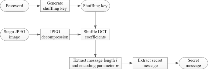
Extraction procedure of F5 steganography
-
2)
Generate a shuffling key from a given password and shuffle the coefficients obtained in step 1.
-
3)
Extract the metadata (matrix encoding parameter c and message length l).
-
4)
Extract the embedded message by matrix decoding.

The following two characteristics of the quantized DCT coefficients will be maintained after embedding messages into an image by F5 steganography (see Fig.3).
-
(i)
The quantized DCT coefficients with larger absolute values appear with lower frequency, so the bins of the quantized DCT coefficients with larger absolute values are smaller.
-
(ii)
As the absolute value of the quantized DCT coefficients increases, the frequency of the DCT coefficient decreases at a smaller rate. For example, the difference between two adjacent bins close to coefficient value 0 is greater than that between two adjacent bins far from coefficient value 0.

Histogram of the quantized DCT coefficients in a JPEG image
The above characteristics mean that the number of 1s in the LSBs of non-zero AC coefficients is greater than the number of 0s.
3 Method—stego key recovery method for F5 steganography
From Figs. 1 and 2, it is clear that the stego key of F5 steganography is composed of the shuffling key and the check matrix of matrix encoding. If one can obtain these two components, then the embedded message can be extracted. The brute force attack method tries all possible shuffling keys and check matrices, so it is highly inefficient. If the check matrix or shuffling key can be obtained before searching for another, then the time complexity could be reduced significantly. Following this thought, this section will present a stego key recovery method for F5 steganography with matrix encoding. The presented method contains two main procedures: recovery of check matrix and recovery of shuffling key, which are described in the following parts.
In order to simplify the description, the following symbols are defined firstly.
-
1)
Let X=x1,x2,…,xN denote the quantized DCT coefficients in the cover image, where N is the number of quantized DCT coefficients in the cover image.
-
2)
Let Y=y1,y2,…,yN denote the quantized DCT coefficients in the corresponding stego image.
-
3)
Let M=m1,m2,…,ml denote the sequence of embedded message bits, where l is the length of message.
-
4)
Let Hw denote the check matrix of matrix encoding used in F5 steganography with parameter w.
-
5)
Let K denote the space of shuffling keys, where |K| is the size of the shuffling key space, and let k0 be the correct shuffling key.
-
6)
Let Mi=(mi,1,mi,2,…,mi,w) denote the ith group of embedded message bits.
-
7)
Let Ci=(ci,1,ci,2,…,ci,W) denote the sequence of bits expressed by the selected ith group of W non-zero AC coefficients.
-
8)
Let Si=(si,1,si,2,…,si,W) denote the sequence of bits expressed by the ith group of W non-zero stego AC coefficients.
3.1 Recovery of check matrix in F5 steganography
During embedding, if F5 steganography modifies a coefficient with an absolute value of 1, one more non-zero AC coefficient is read and added to the buffer to form a new group of W coefficients. F5 steganography does not embed the message into the DC (direct current) coefficients. Therefore, one can compute the estimated capacity with no matrix encoding as follows:
where hDCT denotes the number of quantized DCT coefficients in the cover image, h(0) denotes the number of AC coefficients equal to zero, h(1) denotes the number of AC coefficients with an absolute value of 1, \(\frac {h_{DCT}}{64}\) is the number of DC coefficients, and 0.51h(1) is the estimated loss due to shrinkage.
F5 steganography computes the modified position ai as follows:
where the function bin2dec((b1,b2,…,bw)T) converts the binary vector (b1,b2,…,bw)T to a decimal number \({\sum \nolimits }_{j=1}^{w}b_{j}2^{w-j}, M^{T}_{i}\) and \(C^{T}_{i}\) denote the transpositions of Mi and \(C_{i}, \bigoplus \) denotes the bitwise XOR (exclusive or) operation. If ai=0, the selected ith group of non-zero AC coefficients should remain unchanged. If ai≠0, the aith bit in Ci should be changed to obtain the stego bit sequence. That is,
On the receiving side, F5 steganography decodes the message bits as follows:
From (4), it is apparent that the check matrix Hw is determined by the parameter w and the elements in it. Fortunately, in F5 steganography, the elements in all positions of the check matrix Hw are also determined by the parameter w as follows:
where bit(j,w−i+1) denotes the (w−i+1)th least-significant bit of the value j, 1≤i≤w and 1≤j≤2w−1. For example, when w=2, the check matrix is
and when w=3, the check matrix is
Therefore, the recovery of check matrix in F5 steganography can be viewed as the recognition of the encoding parameter w. Because F5 steganography encodes message bits with as many available coefficients as possible, the parameter w should satisfy the following inequality:
where \(r=\frac {l}{L}\). Therefore, we can adopt a quantitative steganalysis algorithm to estimate the embedding ratio in the stego image, then obtain the parameter w using (8). Currently, many quantitative steganalysis algorithms have been proposed for F5 steganography. For example, Fridrich et al. calibrated the given image to estimate the coefficient histogram of the cover image, and then used a least squares method to estimate the message length l [39]. Luo et al. improved the modification ratio estimation in Fridrich’s algorithm based on relative entropy [40].
It can be found that the probability to successfully recover the check matrix depend on whether the message length can be estimated with error \(e=\hat {l}-l\) in the range \(\left (\frac {w-1}{2^{w-1}-1}L-l, \frac {w}{2^{w}-1}L-l\right ]\). Thus, this further demonstrates that it is necessary to design more accurate quantitative steganalysis algorithm.
3.2 Recovery of shuffling key in F5 steganography
Recovering the shuffling key in F5 steganography involves distinguishing the true shuffling key k0 from the key space. This section describes the principle to recover the shuffling key based on the distribution of the extracted message bits.
Firstly, the following symbols are defined:
-
1)
Let u0 denote the frequency of 0 in the bit sequence extracted from the non-shuffled DCT coefficients;
-
2)
Let u1 denote the frequency of 1 in the bit sequence extracted from the non-shuffled DCT coefficients;
-
3)
Let I(k) denote the bit sequence extracted from the DCT coefficients shuffled by key k;
-
4)
Let p0(k,n) denote the frequency of 0 in the first n bits of I(k);
-
5)
Let p1(k,n) denote the frequency of 1 in the first n bits of I(k).
The difference between the distributions of the message bits extracted by the true and false shuffling keys is analyzed as follows.
-
a)
Statistical characteristics of message bits extracted by the true shuffling key. In F5 steganography, when the embedded message has been encrypted, it should be a stream of pseudo-random bits in which 0 and 1 appear with equal probabilities. Therefore, there should be p0(k0,n)≈p1(k0,n)≈0.5n, where 0<n≤l.
-
b)
Statistical characteristics of message bits extracted by the false shuffling key. When w=1, the matrix encoding degrades to simple LSB embedding. From statistical characteristic (i) of the quantized DCT coefficients, one can infer that there should be more 1s than 0s in the LSBs of the non-zero AC coefficients of the stego image, i.e., u1>u0. When w≥2, one can infer from statistical characteristic (i) that, in all groups of 2w−1 non-zero AC coefficients selected from the non-shuffled DCT coefficients, the groups whose elements’ LSBs are all 1 will appear most frequently. Because the group \(\phantom {\dot {i}\!}(1, 1, \ldots, 1)_{2^{w}-1}\) will be decoded as \(\phantom {\dot {i}\!}H_{w}(1, 1, \ldots, 1)^{T}_{2^{w}-1}=(0, 0, \ldots, 0)^{T}_{w}\), there should be more 0s than 1s in the bit sequence extracted from the non-shuffled DCT coefficients, i.e., u1<u0. Because the secret message bits are pseudo-randomly spread across all non-zero AC coefficients, the distribution of the message bits extracted by the false shuffling key is similar to that of the message bits extracted from the non-shuffled image. Therefore, in the message bits extracted by the false shuffling key k, there should be p1(k,n)=u1,p0(k,n)=u0, and p1(k,n)≠p0(k,n).
For example, when there are 5 coefficients whose LSBs are 1s and 1 coefficient whose LSB are 0s in a JPEG image, all of the possible stego bit sequences are showed in the following Table 1. It can be seen that there are 4 extracted message bit sequences where the number of 0s is more than half of the length.
In a word, the distribution of the message bits extracted by the true shuffling key is different from that extracted by the false shuffling key. Therefore, we can use a non-parametric hypothesis testing to examine whether the message bits extracted by the test shuffling key conform to the distribution of the message bits extracted by the true shuffling key. Namely, the recovery of the shuffling key can be viewed as the testing with following hypothesis:
where F0(x) is the distribution of the bit sequence I(k0) extracted by the true shuffling key k0.
Let f(x) denote the probability function of the distribution F0(x). Because the relative frequencies of 1 and 0 in I(k0) are both approximately equal to 0.5, it holds that
In the first n bits of the bit sequence I(k), the actual frequencies of 0 and 1 are np0(k,n) and np1(k,n), respectively. From (10), the true shuffling key k0 produces theoretical frequencies of 0.5n for both 0 and 1. Thus, when the test shuffling key k is true, Pearson’s theorem implies that the limit distribution of the following statistics is the χ2 distribution with a single degree of freedom:
The probability distribution function of the statistics is
The true shuffling key k0 will generate the small value of t(k,n) which would cause small value of p(k). In contrast, if k is a false shuffling key, the limit distribution of the statistics t(k,n) should not be the χ2 distribution with one degree of freedom and generate a larger value of t(k,n) which would cause large value of p(k). Therefore, we attempt to search for the shuffling key k that generates a small value of t(k,n). Note that the search speed of the shuffling key is related to the number of samples n. Larger values of n will produce more accurate results, but reduce the search speed of the shuffling key. Thus, we need to find an appropriate value of n.
For the given significance level α, the threshold value T(α) of t(k,n) used to test the true and false shuffling keys should satisfy
and the rejection region is (T(α),∞). When the test key is the true shuffling key k0, the corresponding statistics t(k0,n) takes the smallest value over the whole key space and t(k0,n)<T(α). The statistics t(kj,n) of the false shuffling key kj(j≠0) will be larger than T(α). Let Δ=t(kj,n)−T(α)(j≠0) denote the difference between the statistics t(kj,n) of the false key and the threshold value. Then, we obtain
where Δ>0. Thus, the number of bits used should be
It can be seen that there are two extreme cases in (15), viz. the case of the embedding ratio r→1, and the case of the embedding ratio r→0. In these two extreme cases, it is possible failure to recover the shuffling key.
-
1)
As the embedding ratio r→1, the characteristics u0→0.5,u1→0.5 and (15) would cause that n→∞. Thus, the shuffling key would not be successfully recovered because of an insufficient number of samples.
-
2)
As the embedding ratio r→0, if the message length l is less than n, the shuffling key would not be successfully recovered. In the χ2 testing, the number of samples belonging to each class should satisfy 0.5n≥50, so the number of samples used should satisfy
$$ n\geq 100. $$(16)which also means that the message length l should be not smaller than 100 bits.
After shuffling the quantized DCT coefficients, F5 steganography embeds the metadata (matrix encoding parameter w and message length l) in the embedding procedure and extracts the metadata in the extraction procedure. The matrix encoding parameter w is determined by l and L using (8) and the message length l must not exceed L. Table 2 presents the performance results of matrix encoding with different encoding parameters. The value of w must be an integer in the range 1-9. Thus, if the parameter wk extracted by a test shuffling key k does not satisfy this criterion, this key must be false. We can use a quantitative steganalysis algorithm to estimate the embedding ratio l/L, and then obtain the parameter w. If wk≠w, the tested shuffling key k also must be false. Additionally, if the message length lk extracted by shuffling key k is greater than the number of non-zero AC coefficients, the tested shuffling key k also must be false.
3.3 Description of stego key recovery method
In summary, the stego key of F5 steganography, composed of the shuffling key k0 and the check matrix of matrix encoding Hw, can be recovered as follows (seeing Fig.4).
-
1
Decoding: Decode the given stego JPEG image to obtain the quantized DCT coefficients and count the number of non-zero AC coefficients NAC≠0.
-
2
Estimate metadata and recover check matrix: Estimate the message length l using a quantitative steganalysis algorithm, and then determine the matrix encoding parameter w and the check matrix Hw.
-
3
Count frequencies of 0s and 1s extracted from the non-shuffled DCT coefficients: Extract the bit sequence from the non-shuffled DCT coefficients and count the frequency of 0s in the extracted bit sequence, u0, and the frequency of 1s in the extracted bit sequence, u1.
-
4
Scan the shuffling key space: Examine each possible shuffling key k in the shuffling key space K through the following steps.
-
(a)
Shuffle the coefficients obtained in step 1.
-
(b)
Extract the matrix encoding parameter wk and the message length lk.
-
(c)
If wk=w and lk<NAC≠0, add k to the set of candidate shuffling keys, B; otherwise, examine the next possible shuffling key.
-
(a)
-
5
Examine the set of candidate shuffling keys: If there is only one key in B, i.e., |B|=1, the only key is regarded as the recovered shuffling key \(\hat {k_{0}}\).
-
6
Scan the set of candidate shuffling keys: If |B|>1, compute the number of bit samples needed by the given significance level α and difference Δ using (15), n, and then examine each candidate shuffling key k in B through the following steps.
-
(a)
Count the number of 0s and the number of 1s in the first n bits of the bit sequence extracted by the possible shuffling key, i.e., p0(k,n) and p1(k,n).
-
(b)
Compute the statistics t(k,n) using (11).
-
(c)
If t(k,n)≥T(α), delete k from B.
-
(a)
-
7
Re-examine the set of candidate shuffling keys: If |B|=1, the only key in B is regarded as the recovered shuffling key \(\hat {k_{0}}\). If |B|>1, the key in B with the minimum statistics t(k,n) is regarded as \(\hat {k_{0}}\). If |B|=0, return -1 to denote that the process has failed to recover the shuffling key.
-
8
Return result: Return the recovered check matrix Hw and shuffling key \(\hat {k_{0}}\) as the recovered stego key.

Diagram of the proposed stego key recovery method
4 Results and discussion
4.1 Experimental setup
The F5 steganography software was implemented in Java. When the user inputs a password, the password is stored as a string variable. Because the maximum length of string variable is 216−1=65535 bytes in Java, when the password length is d (1≤d≤65535), the cardinality of the shuffling key space is |K|=28d. To reduce the time cost of experiments, the shuffling key was tested in a space of size 106. The “lena.jpg” image with 512 ×512 pixels and a quality factor of 75 was token as the cover image. Then, experiments were performed on a PC (personal computer) with a dual-core CPU (central processing unit), 3 GB (gigabyte) memory, and main frequency of 2.20 GHz (gigahertz), as follows:
-
1)
Pseudo-randomly select a password from the space {“000000”, “000001”, …, “999999”};
-
2)
Estimate the capacity of the cover “lena.jpg” image;
-
3)
According to the embedding ratio r and the estimated capacity, generate a pseudo-random bit sequence;
-
4)
Use the F5 steganography software to embed the generated pseudo-random bit sequence into the cover “lena.jpg” image with the selected password, and then generate the stego “lena.jpg” image;
-
5)
Use the stego key recovery method to recover the stego key from the generated stego image.
4.2 Experimental results and analysis
In the proposed stego key recovery method, the value of Δ is related to the cardinality of the shuffling key space, |K|, and the embedding ratio r. When the value of r is larger, the number of samples required, n, will be higher and the search speed will be slower. Therefore, the value of Δ should be as small as possible. The experiments were performed with different values of Δ, starting from 0 and increasing in steps of 5, until the shuffling key had been identified or the number of samples exceeded the message length. Table 3 presents the experimental results for different embedding ratios, where “-” denotes that the number of samples exceeded the message length and “*” denotes that the value of Δ makes the number of samples equal to the message length.
From the results in Table 3, the following conclusions can be drawn.
-
1)
When the matrix encoding parameter w=1, if the embedding ratio r = 0.85, the stego key cannot be recovered successfully; if the embedding ratio r = 0.67, 0.7, 0.75, and 0.8, the stego key can be recovered successfully. This is because a high embedding ratio in F5 steganography makes the histogram of DCT coefficients shrink significantly. Although we can estimate the capacity from (1), as the embedding ratio r→1, the degree of shrinkage results in large errors of the estimated capacity. For example, in the “lena.jpg” image with a quality factor of 75, when the estimated embedding ratio r = 0.85, the actual embedding ratio is about 0.977. When the estimated embedding ratio r = 0.87, the stego image has been embedded fully. When the embedding ratio is close to 1, i.e., r→1,u0→0.5,u1→0.5, the number of samples required, as computed by (15), then exceeds the message length. A lack of available samples results in a failure to recover the stego key.
-
2)
When the matrix encoding parameter w=2, the stego key can be recovered successfully for various embedding ratios.
-
3)
When the matrix encoding parameter w≥3, the stego key cannot be recovered successfully. The matrix encoding attempts to embed information into more coefficients with fewer modifications, and the modification ratio is
As the matrix encoding parameter w increases, the modification ratio becomes smaller. This smaller modification ratio implies a smaller difference between the stego image and the cover image, and a smaller difference between the distributions of message bits extracted by the true stego key and the false stego key. Thus, more samples are needed to recover the stego key successfully. If the number of samples required exceeds the message length, the lack of available samples results in a failure to recover the stego key. For example, when w=3, the modification ratio is 1/8 and the maximum embedding ratio is 3/7 ≈0.42. In this case, even when all of the extracted bit samples are utilized, this is still less than the number of samples required. Therefore, the stego key cannot be recovered successfully.
In the following, the proposed method is compared with the stego key recovery method proposed by Xu et al. [30] that is denoted as Xu’s method.
-
1)
Comparison between the principles. Xu’s method fits the distributions of the quantized DCT coefficients in the embedding paths generated by the true stego key and false stego keys, whereas the proposed method utilizes the distribution difference between the message bits extracted by the true stego key and false stego keys. Xu’s method does not compute the number of samples required, whereas the proposed method contains a simple method to compute this number.
-
2)
Comparison between the application scopes. Xu’s method is only effective for F5 steganography without matrix encoding, whereas the proposed method is effective for F5 steganography with matrix encoding. Neither Xu’s method nor the proposed method can successfully recover the stego key when the embedding ratio r→1 or r→0. In the following, we compare these two methods in the cases of large embedding ratios and small embedding ratios.
In the case of large embedding ratios, as the embedding ratio r close to 1, there should be large error in the estimated capacity. Thus, the embedding ratio r cannot be too large. For example, in the “lena.jpg” image with a quality factor of 75, when the estimated embedding ratio r=0.87, the stego image has been fully embedded. Therefore, only experimental results for embedding ratios of 0.65, 0.7, 0.75, 0.8, and 0.85 are listed in Table 4. The results show that, when the embedding ratio are 0.75 and 0.8, the proposed method can recover the shuffling key successfully, but the Xu’s method fails. When the embedding ratio r = 0.85, both methods fail. This is because the embedding ratio is computed with a large error in the capacity estimation, and the actual embedding ratio is about 0.977. This is very close to 1, causing a very slight difference between the statistical characteristics along the embedding paths generated by the true shuffling key and the false shuffling key. Therefore, there are insufficient samples available to recover the shuffling key.
Table 4 Experimental results in the cases of large embedding ratios In the case of small embedding ratios, the experimental results are presented in Table 5. The results show that, when the embedding ratios are 0.001, 0.002, and 0.003, both methods fail to recover the shuffling key because too few samples are available. Both methods use χ2 statistics, but the proposed method divides the samples into two categories whereas Xu’s method divides the samples into five categories [30]. In the χ2 testing, each category must contain sufficient samples. Thus, Xu’s method is more likely to fail because of less samples in each category. Therefore, when the embedding ratios are 0.004 and 0.005, Xu’s method fails while the proposed method can recover the shuffling key successfully. Hence, the proposed method outperforms Xu’s method [30].
Table 5 Experimental results in the cases of small embedding ratios -
3)
Comparison between the time complexities. Both Xu’s method and the proposed method must search the given shuffle key space. Therefore, if the shuffling key space is fixed, the time complexities of the two methods are determined by the number of samples required. A larger number of samples would result in higher time complexity. When the numbers of samples required by the two methods are equivalent, Xu’s method should extract n bits for each possible key in the shuffling key space. Its time complexity is n|K|. But the proposed method in this paper need to extract only 31 bits of metadata to determine the set of candidate shuffling keys B, then extract n bits for each candidate shuffling key. Thus, the time complexity of the proposed method is 31|K|+n|B|. Because the cardinality of B is usually much smaller than that of the shuffling key space, the time complexity of the proposed method is usually lower than that of Xu’s method.
As an example, consider the stego “lena.jpg” image with a quality factor of 75 and embedding ratio of r = 0.66 (matrix encoding parameter w = 2). All possible shuffling keys were used to extract the encoding parameter w and the message length l. When the extracted encoding parameter w=1, 2, …, 9, the corresponding shuffling key was added to the set of candidate shuffling keys, B. Figure 5 shows the numbers of keys by which the encoding parameter w=1, 2, …, or 9 were extracted. The examination of encoding parameter reduced the cardinality of the shuffling key space from 106 to 137533. Because the encoding parameter is related to the embedding ratio, matching the encoding parameter to the embedding ratio further reduced the shuffling key space to 15091 keys when w = 2, which is only 1.51% of the whole shuffling key space. Because the message length cannot be greater than the number of non-zero AC coefficients, by excluding the keys that generate such message lengths, i.e., l>NAC≠0, the cardinality of the shuffling key space was reduced to 60, just 0.006% of the whole shuffling key space. Therefore, the time complexity of the proposed method is significantly lower than that of Xu’s method.

Numbers of shuffling keys by which the encoding parameter w=1, 2, …, or 9 were extracted
5 Conclusions
F5 steganography synthesizes matrix encoding and DCT coefficients shuffling, and takes the check matrix of the matrix encoding and a shuffling key as the stego key. However, previous stego recovery methods only work in the absence of matrix encoding. Therefore, this paper proposes a stego key recovery method to recover the check matrix and shuffling key. Firstly, the check matrix of the matrix encoding is recovered based on the embedding ratio estimated by quantitative steganalysis. The shuffling key is then recovered using a χ2 testing and by examining the extracted metadata. Experimental results demonstrate the effectiveness and superiority of the proposed method over the existing stego key recovery method for F5 steganography—Xu’s method.
However, in STC-based steganography, multiple check submatrices are placed next to each other and shifted down by on row to generate the check matrix. The check submatrices could be generated by a key, and the decoded message bits are controlled by not only the check submatrix and stego bit subsequence in the corresponding positions, but also the check submatrices and stego bit subsequences in previous positions. Therefore, the proposed method can not directly applied to the recovery of the stego key for the STC-based steganography. And we will try to find the new property of the bit sequence decoded from the randomly shuffling coefficients to recognize the correct stego key.
Additionally, in the future work, we will try to locate the stego positions by machine learning and searching for similar images [41, 42] and even consider the generation and operation history of the stego image [43–45].
Availability of data and materials
The datasets involved in the current study are available from the corresponding author by reasonable request.
Abbreviations
- JPEG:
-
Joint photographic experts group
- LSB:
-
Least significant bit
- MLSB:
-
Multiple least significant bits
- DCT:
-
Discrete cosine transform
- STC:
-
Syndrome-trellis codes
- HUGO:
-
Highly undetectable stego
- AC:
-
Alternating current
- XOR:
-
Exclusive or
- PC:
-
Personal computer
- CPU:
-
Central processing unit
- GB:
-
Gigabyte
- GHz:
-
Gigahertz
References
Y. Zhang, X. Y. Luo, Y. Q. Guo, C. Qin, F. L. Liu, Multiple robustness enhancements for image adaptive steganography in lossy channels. IEEE Trans. Circ. Syst. Video Technol.30(8), 2750–2764 (2020).
C. Qin, W. Zhang, F. Cao, X. P. Zhang, C. C. Chang, Separable reversible data hiding in encrypted images via adaptive embedding strategy with block selection. Sig. Process.153:, 109–122 (2018).
L. Xiang, Y. Li, W. Hao, P. Yang, X. Shen, Reversible natural language watermarking us-ing synonym substitution and arithmetic coding. Comput. Mater. Continua. 55(3), 541–559 (2018).
T. Qiao, X. Y. Luo, T. Wu, M. Xu, Z. X. Qian, Adaptive steganalysis based on statistical model of quantized dct coefficients for jpeg images. IEEE Trans. Dependable Secur. Comput. (2019). https://doi.org/10.1109/TDSC.2019.2962672.
X. Y. Luo, D. S. Wang, P. Wang, F. L. Liu, A review on blind detection for image steganography. Signal Process.88(9), 2138–2157 (2008).
X. Song, F. Liu, C. Yang, X. Luo, Y. Zhang, in Proceedings of the Third ACM Workshop on Information Hiding and Multimedia Security: 17-19 June 2015, ed. by A. M. Alattar, J. J. Fridrich, N. M. Smith, and P. C. Alfaro. Steganalysis of adaptive JPEG steganography using 2D Gabor filters (ACMPortland Oregon USA, 2015), pp. 15–23.
Y. Ma, X. Luo, X. Li, Z. Bao, Y. Zhang, Selection of rich model steganalysis features based on decision rough set α-positive region reduction. IEEE Trans. Circ. Syst. Video Technol.29(2), 336–350 (2019).
C. Yang, F. Liu, X. Luo, B. Liu, Steganalysis frameworks of embedding in multiple least-significant bits. IEEE Trans. Inf. Forensic. Secur.3(4), 662–672 (2008).
C. Yang, F. Liu, X. Luo, Y. Zeng, Pixel group trace model-based quantitative steganalysis for multiple least-significant bits steganography. IEEE Trans. Inf. Forensic. Secur.8(1), 216–228 (2013).
Y. Kang, F. Liu, C. Yang, X. Luo, T. Zhang, Color image steganalysis based on residuals of channel differences. Comput. Mater. Continua. 59(1), 315–329 (2019).
L. Xiang, G. Guo, J. Yu, V. S. Sheng, P. Yang, A convolutional neural network-based linguistic steganalysis for synonym substitution steganography. Math. Biosci. Eng.17(2), 1041–1058 (2019).
A. D. Ker, R. Böhme, in Proceedings of SPIE 6819, Security, Forensics, Steganography, and Watermarking of Multimedia Contents X: 27 January 2008, ed. by E. J. D. III, P. W. Wong, J. Dittmann, and N. D. Memon. Revisiting weighted stego-image steganalysis (SPIESan Jose, CA, USA, 2008), pp. 27–31.
A. D. Ker, in Proceedings of Third International Symposium on Information Assurance and Security: 29-31 August 2007, ed. by N. Zhang, A. Abraham, Q. Shi, and J. Thomas. A weighted stego image detector for sequential lsb replacement (IEEEManchester, UK, 2007), pp. 453–456.
A. D. Ker, I. Lubenko, in Proceedings of SPIE 7254, Media Forensics and Security: 18-22 January 2009, ed. by E. J. D. III, J. Dittmann, N. D. Memon, and P. W. Wong. Feature reduction and payload location with WAM steganalysis (SPIESan Jose, California, USA, 2009), p. 72540.
T. T. Quach, Optimal cover estimation methods and steganographic payload location. IEEE Trans. Inf. Forensic Secur.6(4), 1214–1222 (2011).
T. T. Quach, in Proceedings of SPIE 9028, Media Watermarking, Security, and Forensics: 2-6 February 2014, ed. by A. M. Alattar, N. D. Memon, and C. D. Heitzenrater. Cover estimation and payload location using Markov random fields (SPIESan Francisco, California, USA, 2014), p. 90280.
X. Gui, X. Li, B. Yang, in Proceedings of Nineteenth IEEE International Conference on Image Processing: 30 September-3 October 2012, ed. by E. Saber. Improved payload location for LSB matching steganography (IEEEOrlando, Florida, USA, 2012), pp. 1125–1128.
T. T. Quach, Extracting hidden messages in steganographic images. Digit. Investig.11(Suppl 2), 40–45 (2014).
C. Yang, F. Liu, S. Ge, J. Lu, J. Huang, Locating secret messages based on quantitative steganalysis. Math. Biosci. Eng.16(5), 4908–4922 (2019).
J. Wang, C. Yang, P. Wang, X. Song, J. Lu, Payload location for JPEG image steganography based on co-frequency sub-image filtering. Int. J. Distrib. Sensor Netw.16(1), 1550147719899569 (2020).
T. T. Quach, in Proceedings of SPIE 8303, Media Watermarking, Security, and Forensics: 22-26 January 2012, ed. by N. D. Memon, A. M. Alattar, and E. J. D. III. Locatability of modified pixels in steganographic images (SPIEBurlingame, California, USA, 2012), p. 83030.
C. Yang, J. Wang, C. Lin, H. Chen, W. Wang, Locating steganalysis of LSB matching based on spatial and wavelet filter fusion. Comput. Mater. Continua. 60(2), 633–644 (2019).
W. M. Zhang, J. F. Liu, L. S. Q, Approaches for recovering key of LSB steganography. Acta Sci. Nat. Univ. Sunyatseni. 44(3), 29–33 (2005).
J. Fridrich, M. Goljan, D. Soukal, in Proceedings of SPIE 5306, Security, Steganography, and Watermarking of Multimedia Contents VI: 18-22 January 2004, ed. by E. J. D. III, P. W. Wong. Searching for the stego-key (SPIESan Jose, California, USA, 2004), pp. 70–82.
J. Fridrich, M. Goljan, D. Soukal, T. Holotyak, in Proceedings of SPIE 5681, Security, Steganography, and Watermarking of Multimedia Contents VII: 16-20 January 2005, ed. by E. J. D. III, P. W. Wong. Forensic steganalysis: determining the stego key in spatial domain steganography (SPIESan Jose, California, USA, 2005), pp. 631–642.
W. M. Zhang, L. S. Q, J. F. Liu, Extracting attack to LSB steganography in spatial domain. Chin. J. Comput.30(9), 1625–1631 (2007).
J. F. Liu, Y. G. Tian, T. Han, C. F. Yang, L. W. B, LSB steganographic payload location for JPEG-decompressed images. Digit Signal Process.38:, 66–76 (2015).
J. Liu, Y. Tian, T. Han, J. Wang, X. Luo, Stego key searching for LSB steganography on JPEG decompressed image. Sci. China Inf. Sci.59(3), 032105 (2016).
C. Yang, X. Luo, J. Lu, F. Liu, Extracting hidden messages of MLSB steganography based on optimal stego subset. Sci. China Inf. Sci.61:, 119103 (2018).
C. Xu, J. Liu, J. Gan, X. Luo, Stego key recovery based on the optimal hypothesis test. Multimed. Tools Appl.77(14), 17973–17992 (2018).
J. Liu, J. Gan, J. Wang, C. Xu, X. Luo, Efficient stego key recovery based on distribution differences of extracting message bits. J. Real-Time Image Proc.16(3), 649–660 (2019).
W. M. Zhang, S. Q. Li, J. F. Liu, Analysis for the equivalent keys of steganographic scheme CPT. Acta Electron. Sin.35(12), 2258–2261 (2007).
J. Y. Chen, Y. F. Zhu, W. M. Zhang, J. F. Liu, Chosen-key extracting attack to random LSB steganography. J. Commun.31(5), 73–80 (2010).
J. Chen, J. Liu, W. Zhang, H. Liu, X. Zhao, Cryptographic secrecy analysis of matrix embedding. Int. J. Comput. Intell. Syst.6(4), 639–647 (2013).
X. Luo, X. Song, X. Li, W. Zhang, J. Lu, C. Yang, F. Liu, Steganalysis of HUGO steganography based on parameter recognition of syndrome-trellis-codes. Multimed. Tools Appl.75(21), 13557–13583 (2016).
J. Gan, J. Liu, X. Luo, C. Yang, F. Liu, Reliable steganalysis of HUGO steganography based on partially known plaintext. Multimed. Tools Appl.77(14), 18007–18027 (2018).
A. Westfeld, in Proceedings of Fourth International Workshop on Information Hiding: 25-27 April 2001, ed. by I. S. Moskowitz. High capacity despite better steganalysis (F5-a steganographic algorithm) (SpringerPittsburgh, PA, USA, 2001), pp. 289–302.
J. Fridrich, Steganography in digital media—principles, algorithms, and applications (Cambridge University Press, Cambridge, 2009).
J. Fridrich, M. Goljan, D. Hogea, in Proceedings of Fifth International Workshop on Information Hiding: 7-9 October 2002, ed. by F. A. P. Petitcolas. Steganalysis of JPEG images: breaking the F5 algorithm (SpringerNoordwijkerhout, The Netherlands, 2002), pp. 310–323.
X. Luo, F. Liu, C. Yang, S. Lian, D. Wang, On F5 steganography in images. Comput. J.55(4), 447–456 (2012).
L. Xiang, G. Zhao, Q. Li, W. Hao, F. Li, TUMK-ELM: a fast unsupervised heterogeneous data learning approach. IEEE Access. 6:, 35305–35315 (2018).
L. Xiang, X. Shen, J. Qin, W. Hao, Discrete multi-graph hashing for large-scale visual search. Neural. Process. Lett.49(3), 1055–1069 (2019).
J. Wang, T. Li, X. Luo, Y. Q. Shi, R. Liu, S. K. Jha, Identifying computer generated images based on quaternion central moments in color quaternion wavelet domain. IEEE Trans. Circ. Syst. Video Technol.29(9), 2775–2785 (2018).
J. Wang, H. Wang, J. Li, X. Luo, Y. Q. Shi, S. K. Jha, Detecting double jpeg compressed color images with the same quantization matrix in spherical coordinates. IEEE Trans. Circ. Syst. Video Technol.30(8), 2736–2749 (2020).
T. Qiao, R. Shi, X. Luo, M. Xu, N. Zheng, Y. Wu, Statistical model-based detector via texture weight map: application in re-sampling authentication. IEEE Trans. Multimed.21(5), 1077–1092 (2019).
Acknowledgements
Thanks to the editor and anonymous reviewers for their helpful comments and valuable suggestions.
Funding
This work is supported by the National Natural Science Foundation of China (Grant Nos. U1804263, 61772549, 61872448).
Author information
Authors and Affiliations
Contributions
Authors’ contributions
All authors took part in the discussion of the work described in this paper. The first author (JL) proposed the idea and designed the algorithm. The second author (CY) organized the thoughts and wrote the paper. The third author (JW) carried out the experiments of the paper and analyzed the time complexity of the proposed method. The fourth author (YS) analyzed the experimental results and revised the paper. All author(s) read and approved the final manuscript.
Authors’ information
Jiufen Liu is currently a professor of Zhengzhou Science and Technology Institute. She received her B.S. and M.S. degrees from Henan University, Kaifeng, China, in 1985 and 1990, respectively. She received her Ph.D. degree from Zhejiang University, Hangzhou, China, in 2001. Her research interests include steganography and steganalysis.
Chunfang Yang is currently an associate professor of Zhengzhou Science and Technology Institute. He received his MA and PhD degrees in computer science and technology from Zhengzhou Information Science and Technology Institute, Zhengzhou, China, in 2008 and 2012, respectively. His research interest includes image steganography and steganalysis technique.
Junchao Wang is a MA degree candidate for applied mathematics of Zhengzhou Science and Technology Institute. He received his B.S. degree in applied mathematics from National University of Defense Technology. His research interest includes image steganalysis technique.
Yanan Shi is currently a Lecturer of Zhengzhou Science and Technology Institute. She received his MA degree in applied mathematics from Zhengzhou Information Science and Technology Institute, Zhengzhou, China, in 2008. His research interest includes cryptology and network security.
Corresponding author
Ethics declarations
Competing interests
The authors declare that they have no competing interests.
Additional information
Publisher’s Note
Springer Nature remains neutral with regard to jurisdictional claims in published maps and institutional affiliations.
Rights and permissions
Open Access This article is licensed under a Creative Commons Attribution 4.0 International License, which permits use, sharing, adaptation, distribution and reproduction in any medium or format, as long as you give appropriate credit to the original author(s) and the source, provide a link to the Creative Commons licence, and indicate if changes were made. The images or other third party material in this article are included in the article’s Creative Commons licence, unless indicated otherwise in a credit line to the material. If material is not included in the article’s Creative Commons licence and your intended use is not permitted by statutory regulation or exceeds the permitted use, you will need to obtain permission directly from the copyright holder. To view a copy of this licence, visit http://creativecommons.org/licenses/by/4.0/.
About this article

Cite this article
Liu, J., Yang, C., Wang, J. et al. Stego key recovery method for F5 steganography with matrix encoding. J Image Video Proc. 2020, 40 (2020). https://doi.org/10.1186/s13640-020-00526-2
Received:
Accepted:
Published:
DOI: https://doi.org/10.1186/s13640-020-00526-2