

Abstract
This paper presents quantitative measurements of the N2 Gladstone–Dale constant and scalar polarizability in non-equilibrium conditions, created by a nanosecond pulsed discharge at a pressure of 90 Torr. Optical path differences and spatially varying refractive index profiles are obtained by temporally-resolved Mach–Zehnder interferometry. Spontaneous Raman scattering spectroscopy is used to investigate the highly non-equilibrium vibrational population and to measure the N2( ) vibrational temperature and rotational temperature in the discharge afterglow region. The local gas density is inferred from the rotational temperature with isobaric conditions at long time delays ranging from 10 to 500 µs after initiating the pulsed discharge. The non-equilibrium effects on the N2 Gladstone–Dale constant and scalar polarizability are reported within a rotational temperature ranging from 300 to 1000 K. To the best of our knowledge, this is the first time the refractivity of gas has been measured under non-equilibrium conditions in a pulsed discharge afterglow.
Export citation and abstract BibTeX RIS
1. Introduction
The electric dipole polarizability  (hereafter simply polarizability) is defined as the ratio of the induced dipole moment of an atom or molecule to the external electric field [1]. It determines the essential optical properties of atomic and molecular gases such as the refractive index and Rayleigh scattering cross-section [2, 3], with mean optical properties determined by averages over different species, molecular orientations, and internal degrees of freedom [4]. Hence, the thermochemical state of gas molecules (i.e. translational energy, density, and excitation level) is directly related to the mean polarizability and refractive index. In many common environments, such as low-speed gas flow, internal excitation and chemical reactions do not contribute to spatial variation in the gas refractivity. In this regime, optical distortions are produced only by gradients of the density field inside flow structures such as a turbulent boundary layer [5]. By contrast, environments such as hypersonic flight [6–9], reentry [10], laser gain media [11], and pulsed electrical discharges [12] produce conditions of thermal non-equilibrium that can appreciably alter the mean polarizability [13], leading to a higher refractive index expected based on the translational temperature alone. Neglecting the non-equilibrium effects on polarizability can result in systematic errors in quantitative measurements, for example, by artificially reducing the inferred gas density. In the context of beam propagation, larger variations in the refractive index can result in larger optical effects, such as laser beam distortion, absorption, and steering, than otherwise expected. Improving the understanding and prediction of the refractivity of non-equilibrium gases will contribute to improved models of optical propagation through such media, which are critical for analysis and interpretation of experimental measurements such as interferometry [14, 15], Schlieren [16, 17], shadowgraph [18–21] and wavefront sensing. Moreover, such improvements can impact the precision of any sensors that are sensitive to optical distortion, such on-board hypersonic sensors, free-space optical and laser communication, airborne LIDAR, and (counter) directed energy systems.
In the last few decades, the temperature dependence of the polarizability has been widely investigated [22]. The experimental work shows an approximately 1% increase per 1000 K of the mean polarizability in diatomic molecules (H2, N2, O2, and CH4) under thermal equilibrium conditions [23–26]. Direct calculation of the polarizability and its temperature dependence has also been obtained based on molecular dynamics theory [4]. In addition, the contribution to molecular polarizability from vibrational excitations has been theoretically investigated in recent years [27–29], revealing that the vibrational-excited population has appreciable effects on the averaged dipole moment and static polarizability for some diatomic molecules. Model validation requires the experimentalist to obtain several datasets simultaneously, including the gas density, rotational and vibrational temperatures, and refractive index. Hence, it is desirable and essential to experimentally study the non-equilibrium effect on the refractive index and the scalar polarizability, which benefits both the practical applications and theoretical modeling studies [30, 31].
In a previous paper [13], we have theoretically studied the polarizability of nitrogen and oxygen and predicted the influence of non-equilibrium on optical effects. 1%–5% (at moderate gas temperature) and around 10% (at high temperature) changes of the scalar polarizability are predicted in gas molecules (N2 and O2) due to the vibrational and translational population variations. In this work, we experimentally investigate and quantify the impact of non-equilibrium conditions on the mean polarizability and refractive index in a pulsed discharge afterglow. Directly measuring the non-equilibrium refractivity necessitates several independent measurements of the thermo-optical state of the gas. Much of this work is therefore devoted to the application and analysis of two diagnostic techniques: interferometry and spontaneous Raman scattering. The non-equilibrium environment itself has been generated by a pulsed electrical discharge, a technique which is widely used to generate vibrational non-equilibrium conditions [12].
The remainder of the paper is organized as follows: section 2 presents the experimental apparatus for the nanosecond pulsed discharge generation (section 2.1), Mach–Zehnder interferometry setup for the refractive index measurement (section 2.2), and spontaneous Raman scattering spectroscopy for gas temperature and non-equilibrium characterization (section 2.3); section 3 discusses the detail of the experimental implementation and processing of interferometry data (section 3.1), the rotational and vibrational temperature (section 3.2), and extraction of the Gladstone–Dale constant and scalar polarizability (section 3.3). In section 3.4, experimental measurements of the mean polarizability are compared with the semi-classical model described in previous works; section 4 ends with concluding remarks.
2. Experimental setup
2.1. Discharge setup
A controllable and reproducible range of non-equilibrium gas conditions is produced in quiescent N2 gas flow through the application of a nanosecond pulsed electrical discharge. The detailed experimental setup has been described elsewhere [32] and is summarized in the following. Briefly, the discharge is initiated by releasing the energy stored in a high voltage ceramic capacitor by the laser-triggered spark gap (LTSG) technique [33, 34]. In this approach, an external laser-produced plasma controls the timing of the energy delivery from the capacitor to the discharge cell. The LTSG jitter time was investigated in the previous work, and was found to be  20 ns and
  5 ns in pure nitrogen and air conditions, respectively. Typical profiles of voltage, current, power, and energy are shown in figure 1 during the pulsed discharge generation in a nitrogen gas flow inside the discharge cell. Specifically, LTSG triggers the first voltage drop from 7.2 to 4 kV (−20 to 0 ns) outside the cell. The second voltage drop from 4 to 0 kV (0–80 ns) corresponds to the generation of plasma inside the cell. The optical emission (subplot shown in figure 1) is used to infer the shape and volume of the pulse discharge. Based on the profiles of voltage and current, the energy deposited in the nitrogen gas flow is found to be 0.3 mJ, while about 0.17 mJ is dissipated in the LTSG. The gas pressure in the discharge cell is set at 90 Torr (∼12 000 Pa) with a nitrogen gas flow rate of 1 slm (standard liter per minute). The local gas flow speed is estimated to be 2.7 m s−1, which is sufficient to ensure the local test region fully refreshes after each discharge pulse with the system operating at a repetition rate of 10 Hz.
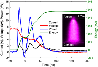
Figure 1. Typical temporal profiles of voltage, current, power, and energy during the pulsed discharge generation. The subplot shows the optical emission from the N2 pulsed discharge.
Download figure:
Standard image High-resolution image2.2. Mach–Zehnder interferometry diagnostics
Mach–Zehnder interferometry is applied to measure the refractive index under non-equilibrium conditions quantitatively. The experimental setup of the Mach–Zehnder interferometer is shown in figure 2. A He–Ne laser source ( 632.8 nm, TEM00 > 95%) is employed with linear polarization and a power of 20 mW. The laser source with a diameter (1 e−2) of 0.7 mm is first attenuated by an iris (I1, Aperture: 0.8 mm), creating an Airy disc. A spatial filter system is then used to suppress the fringes and expand the central maximum (approximately Gaussian spot) up to 20 mm in diameter utilizing an iris (I2, Aperture: 200 µm) and a telescope set F1(f = 100 mm) and F2 (f = 750 mm). Two beam splitters (BS1 and BS2, Thorlabs CCM1-BS013) and two reflector mirrors (M1 and M2, Thorlabs PF10-03-P01) assemble a rectangular optical arrangement. The collimated beam is first divided into two legs by a beam splitter (BS1). One beam passes through the plasma region and the second beam is traveling through room air as a reference leg. The two legs combine at the second beam splitter (BS2), so the interference fringe pattern is formed and recorded by an externally-triggered and time-gated camera. The single-shot interference fringe patterns are acquired at different time delays ranging from −5 to 500 µs. Two hundred interference images are recorded at each time delay after the start of the pulsed discharge while 500 inference images are recorded at
  5 µs (before the start of pulsed discharge) as the reference database. The spatial intensity profile of each leg is also obtained by blocking the light on each leg, which is used to normalize the raw interference image and minimize the influence due to the change/fluctuation of the light source. A typical image of interference fringe pattern (raw data, time delay = 10 µs) is shown in figure 2 and the data analysis procedure and refractive index measurement are described in section 3.1.
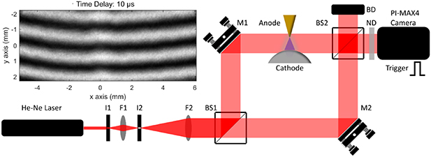
Figure 2. Experimental arrangement of Mach–Zehnder interferometry. I1 and I2 are irises, F1 and F2 work together as a telescope, BS1 and BS2 are beam-splitters, M1 and M2 are reflector mirrors, ND is a neutral density filter, used to control the signal dynamic range of the ICCD camera. The subplot at the top left shows a typical image of interference pattern at a time delay of 10 µs.
Download figure:
Standard image High-resolution image2.3. Spontaneous Raman scattering diagnostics
Spontaneous Raman scattering is an inelastic scattering process between photons and molecules, which was discovered by Raman in 1928. It is essentially an instantaneous process occurring on the time scale of picosecond and benefited by higher incident laser frequency (fourth power dependence) [2]. The great advantage of spontaneous Raman spectroscopy (SRS) is that it is applicable to all molecules, which have at least one vibrational-rotational mode, enabling to provide quantitative, robust, and spatially-resolved measurements. However, due to the weak intensity of SRS, most applications must be performed with long-time signal integration and not amenable to single-shot measurement under low-pressure environments [35]. Recently, high-speed two-dimensional SRS imaging has been demonstrated at elevated pressure. Both the extended pulse width and high gas density environment favor the multi-dimensional, multi-species, high-speed spontaneous Raman scattering [36]. Toward the SRS application in a low-density environment, the cavity-enhanced technique has been recently developed to perform point measurements using a low-power continuous-wave (CW) laser source with an amplification factor of 5900 [37]. Such an approach is capable of performing temporally and spatially resolved Raman measurements for combustion and plasma diagnostics. These two representative works are pursuing critical conditions for SRS applications along with the development of laser technology.
In the current work, the local gas temperature, density, as well as non-equilibrium population in the pulse discharge region are characterized by SRS. Long-time signal integration is applied in this experiment due to the weak SRS signal as mentioned above. The detail of the experimental SRS apparatus has been given in a previous work [32], which mainly investigated the space and time evolution of N2 vibrational non-equilibrium in N2 and air nanosecond discharge afterglow. In this work, the rotational and vibrational temperatures have been simultaneously measured by the SRS technique. Both the whole spectral fitting method and Boltzmann plot fitting method have been used to extract the temperature values from the spectrum. The details are discussed in section 3.2.
3. Results and discussions
3.1. Optical path difference (OPD) and phase shift
In order to determine the changes in the optical path length resulting from the non-equilibrium gas in the pulsed discharge, the interferometer compares one beam traversing through the plasma region with a second beam traversing through room air. The resulting fringe pattern conveys information regarding the difference in two beam paths, or the *** OPD. This can be recast as an optical wave-front distortion, qualified by a phase delay  , which is related to OPD by
where  is the probe laser wavelength. The OPD is also related to the index of refraction by,
where  is the refractive index and
  is the physical path length. The refractive index
  both depends on the gas density and scalar polarizability according to the Lorentz–Lorenz relation, which for dilute gases is approximately given by:
where  is the gas number density,
  is the vacuum permittivity, and
  is the scalar polarizability. In order to obtain
  from the measurement of refractive index
  , we must quantitatively know the gas condition, including gas number density
  , rotational temperature
  and vibrational temperature
  . These details are discussed in sections 3.2 and 3.3. It is important to note that the phase delay has been measured in the pulse discharge afterglow condition starting at a time delay of 10 µs. During the generation of plasma, the ionization degree is on an order of 10–4 with the electron number density on an order of 1015 cm−3. Similar SRS experimental studies were performed previously in both air (1 atm) [38] and pure nitrogen (100 Torr) [39] with the peak density of free electrons on the order of ∼1014–1015 electrons per cm3 during the plasma generation. Due to the high-pressure gas condition in the afterglow, electron density and electron temperature significantly decreased within one microsecond mainly through the dissociative recombination and three-body recombination of electrons with molecular ions [40]. Hence, the effect of dissociated, ionized species, and electrons on the refractive index are ignored after 10 µs in the current work.
The phase delay  is extracted from the interferogram by measuring the location of fringes captured on a camera as shown in figure 3. The interference images are acquired with a time delay ranging from
  5 to 500 µs. The phase shift is not detectable until 2–4 µs delay after the pulsed discharge. As shown in figure 3, the phase shift has an offset from the centerline of the electrodes (
 mm) due to the N2 gas flowing through the discharge cell. It is worth noting that the interference pattern oscillates shot-to-shot due to the physical vibration, room temperature fluctuation, and laser system variation. To reduce the noise generated by these influences, 500 reference images (without plasma excitation, time delay at
  5 µs) are taken as a database. Specifically, the fringe pattern outside the discharge (in the quiescent gas region) is used as a reference. A comparison with the appropriate reference interferogram is obtained by automatically finding the best (least squares) match in the reference database. Consequently, the phase shift around the discharge region can be calculated through the fringe shift (offset) between the selected image and the reference image.
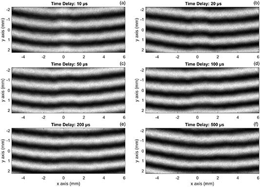
Figure 3. The interference fringe images captured at different time delays after the pulsed discharge. The x-axis indicates the radial distance from the centerline of the electrodes, and the y-axis indicates the vertical distance between the electrodes (top: anode, bottom: cathode). The electrodes gap is ∼5 mm.
Download figure:
Standard image High-resolution imageFigure 4 shows the spatiotemporal distribution of phase delay  and index of refraction (i.e.
  ) at time delays ranging from 10 to 500 µs. The experimental data of phase delay at the center of electrodes (
 mm in figure 3) is extracted from the interference fringes. Two hundred single-shot results are averaged and shown in figure 4, assuming that the spatial distribution is axially symmetric. Instead of directly using Abel's inversion to extract the refractive index from the line-integrated phase delay profile, which is very sensitive to noise, the radial distribution of the refractive index is first initialized as a Gaussian function. The width and amplitude of the Gaussian function are automatically adjusted through the iterative least-squares fitting procedure to find the best fit of the line-of-sight phase delay profile (red lines in figure 4). The index of refraction is analytically solved after the fitting process, which is shown as blue lines in figure 4. The signal-to-noise ratio (SNR) of the phase delay is ∼10 with a standard deviation of 50 mrad. Given a wavelength of
  and a typical discharge afterglow (optical path
  = 2 mm), the minimum observable value for the refractive index change is ∼2.5
  10−6 based on equations (1) and (2). Considering the refractive index (
 3.25
3.25 10−5) at the initial condition (i.e. 90 Torr, 300 K), this value corresponds to a relative error of ∼10%. With the current interferometry setup, the center part of the interference pattern has a relatively higher SNR compared to the edges. Hence, we find the lower SNR values and significant errors at
  5 to
5 to  6 mm shown in figure 4. In the central region, reduced scatter in the data suggests a relative error closer to ∼4%.
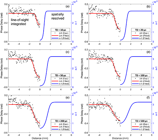
Figure 4. Spatiotemporal distributions of phase delay and refractive index in pulsed discharge afterglow. The phase shift is the line-of-sight integrated result (on the left), and the fitted refractive index (on the right) is spatially-resolved least-square fit result by comparing the experimental data with the fitted curve of phase delay. Note: the distance scale for the RHS is the radial distance (spatially resolved) while that on the LHS is the distance normal to the direction of the laser beam (line-of-sight integrated).
Download figure:
Standard image High-resolution image3.2. Vibrational and rotational temperature
The significant changes of the refractive index in the discharge region depend on both the gas density and non-equilibrium conditions. Here, spontaneous Raman scattering spectroscopy is applied to characterize the non-equilibrium states ( ) and to obtain the quantitative rotational temperature distribution (
 ) and gas density information (
 ). These parameters are used to calculate the gas density
  , Gladstone–Dale constant
  , and scalar polarizability
  under the assumption of isobaric conditions at the longest time delays. Spontaneous Raman scattering spectroscopy has been recently used for studies of nanosecond pulse discharges in air [38, 41] and nitrogen [39]. Similar to these studies, here we present the temporally and spatially resolved measurements of N2 vibrational temperature and rotational temperature at a pressure of 90 Torr with the time delay ranging from 100 ns to 500 µs after the pulsed discharge.
SRS signals are collected from the focused laser beam ( : 1000 mm, beam waist: ∼75 µm, depth of focus: ∼8 mm) near the center of the pulsed discharge afterglow region as shown in figure 5. Within the ∼14 mm measurement range, the laser beam (e.g. intensity and focusing) has no significant change due to the loose focusing (
 : 1000 mm). Figure 5 shows a series of spatially-resolved spontaneous Raman spectra in N2 discharge afterglow at different time delays ranging from 10 to 500 µs. The initial pressure and temperature are 90 Torr and 300 K, respectively. Each spectrum shown in figure 5 is an averaged and background-subtracted image through a three-step data processing procedure. First, a 200-shot on-chip accumulation setting is selected on the ICCD camera to obtain a single averaged image. A total of five images are acquired at each time delay. Second, the same procedure is applied at the same time delay with no probe beam, obtaining five reference images with plasma emission only. Third, each image in the first step is subtracted by a reference image in the second step, providing five 'background-subtracted' images. The average result of these five images is shown in figure 5. The current procedure is a tradeoff between the SNR and signal collection time. The purpose of taking multiple frames is to filter out the saturated pixels due to random stray light or Mie scattering during post-processing. The spectrometer slit width is set at 10 µm and the camera gate width is fixed at 30 ns. At a time delay of 10 µs, high vibrational levels (up to
  ) are observed off-axis. The low Raman signal on-axis indicates a reduced density and likely the high rotational temperature
  . At a later time delay (i.e. 500 µs), the molecules have repopulated the lower vibrational levels at the center of discharge region as show in figure 5(f).
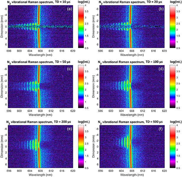
Figure 5. Spatiotemporal Raman spectra of N2( ) in the pulsed discharge afterglow along the laser beam. The laser beam is passing through the center of two electrodes (∼2.5 mm from anode and cathode). The y-axis corresponds to the spatial dimension, and the x-axis corresponds to the spectral dimension. Experimental data are obtained at different time delays ranging from 100 ns to 500 µs. Six Raman spectra are shown here corresponding to the experimental results of the refractive index at the same time delays. The signal intensity uses a logarithmic scale.
Download figure:
Standard image High-resolution imageThe rotational temperature and vibrational non-equilibrium of N2 in the discharge afterglow are obtained by fitting the experimental data with the theoretical Raman scattering spectra. The N2 Raman Q-branch vibrational-rotational spectra are modeled, including the Q-branch line intensity, the non-equilibrium population, and the anharmonicity effect. The Q-branch line intensity is given by [35, 42]:
where  and
and  are the Planck constant and the vacuum permittivity,
  and
and  are the vibrational and rotational state of N2 molecules,
  is the isotropic dipole polarizability,
  is the polarizability anisotropy,
  and
and  are the laser wavenumber and the Q-branch Raman shift, respectively,
  is a Placzek–Teller coefficient [35] and
  is the incident laser irradiance. The expectation values
  are the isotropic and anisotropic matrix elements of the polarizability tensor calculated by [43]:
 and
and  are the N2 molecular constants [44].
  and
and  are parameters for the anharmonicity corrections [43]. The N2 molecular population,
  in the state (
 ,
,  ) is described by rotational temperature
  and vibrational temperature
  due to the non-equilibrium population in the discharge afterglow by a two-temperature Boltzmann factor,

where  is the total number of N2 molecules, and
  is the nuclear spin degeneracy.
  and
and  are the vibrational and rotational energy levels in the state (
 ), respectively.
  and
and  are the vibrational and rotational partition functions. Hereafter, we assume that the gas temperature
  and the rotational temperature
  are equal due to the fast rotational-translation transfer [45, 46]. The vibrational-rotational interaction effects and Herman-Wallis factors are not included in our model, which has a slight effect on the Raman line intensities due to the moderate spectral resolution in the experiment [38].
Two sets of experimental data are employed to verify the Raman spectrum model as shown in figure 6. The experimental data (green line) in the left plot is acquired in a H2–O2–N2 flame with mole ratios of 4/1/4 [47] and the experimental data set (green '+' dots) in the right plot is taken in a H2-air stoichiometric flame [48]. The model shows good agreement with the experimental data in flame conditions under the thermal equilibrium state ( ). The non-equilibrium conditions (i.e.
  ) are also illustrated in figure 6 (on the left). Specifically, with lower rotational temperature, fewer molecules populate the high energy levels inferred from the significant signal decay on the left-wing side of the spectrum. Voigt function interpolated by the Whiting's approximation [49] is applied in the modeling as the instrument function of the spectrometer system.
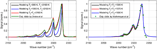
Figure 6. Raman vibrational-rotational spectrum model verification based on the experimental data in flame environments.
Download figure:
Standard image High-resolution imageWith the verified Raman model, the temperature information is extracted by the whole spectral fitting method. Figure 7 shows a typical Raman spectral fitting and temperature extraction result in the N2 discharge afterglow at the time delay of 100 µs at two different positions. The left plot shows the spectrum near the center of the plasma region, while the right one shows the spectrum obtained at 1 mm offset from the radial center of the plasma region. The best-fit result between the experimental data and the Raman model extracts the rotational temperature and the vibrational temperatures with the uncertainty of ∼±100 K, which is mainly determined by the SNRof N2 spectra. For instance, the high rotational temperature (figure 7 on the left) reduces local gas density, which profoundly affects the signal levels of Raman scattering in the local region. At later time delays in the discharge afterglow the uncertainty is significantly reduced due to recovery of the local gas density.

Figure 7. Typical Raman spectral fit and temperature extraction in N2 discharge afterglow at the time delay of 100 µs (left: near the center of the plasma region; right: ∼1 mm radial displacement from the plasma center).
Download figure:
Standard image High-resolution imageBesides the whole spectral fitting method, the Boltzmann plot method has also been used in this work. Figure 8 shows the five-pixel-binned N2 spectrum at the center of the discharge afterglow region with a time delay of 1 µs. Compared to the strong vibrational branches, the rotational lines are not spectrally resolved. Hence, Gumbel distribution function is used for the curve fitting of the individual vibrational branch with an asymmetric shape capturing the rotational population. The area under each band divided by  yields the relative population
  of each vibrational level as shown in the Boltzmann plot (figure 8 subplot). The bimodal structure [46] shown here indicates a non-equilibrium population of the vibrational modes. At the time delay of 1 µs the first level vibrational temperature
  is 1796 ± 50 K and the higher-level vibrational temperature
  is 5117 ± 200 K. With the redistribution of vibrational population at later time delays (10–500 µs), the difference between
  and
and  rapidly decreases with no significant bimodal structure observed after 10 µs. However, the slight difference between
  and
and  exists in the current N2 plasma afterglow environment for a few hundreds of microseconds.

Figure 8. Spectral fitting of each vibrational band for the relative N2 vibrational population measurement. (Subplot) The Boltzmann plot for the vibrational temperature calculation.
Download figure:
Standard image High-resolution imageWith the probe beam passing through the discharge afterglow, the scattered Raman signal along the beam path provides spatially-resolved profiles of temperature. Figure 9 (on the left) illustrates the spatial (radial) distributions of the vibrational temperatures (i.e.  ,
,  ) and the rotational temperature
  at the time delay of 100 µs. The left half part of the plot shows the spatial distribution of the vibrational temperatures
  and
and  by using Boltzmann plot method. The right part shows the spatial-resolved temperature information (
 ,
,  , and
, and  ) by applying the whole spectral fitting method. The fitting results show a good agreement with the two different approaches with a discrepancy of less than
  5%. Laser Rayleigh scattering has also been conducted for the measurement of gas temperature in the pulse discharge afterglow with the result as shown in figure 9 (on the right). Good agreement on gas temperature is confirmed by comparing with Laser Raman scattering and Laser Rayleigh scattering measurements. The discrepancy near the center of the plasma region is mainly due to the low gas number density. Both Rayleigh and Raman have their advantages in the experiment: Rayleigh scattering has a larger differential cross section (giving higher scattering intensity) while Raman scattering simultaneously offering both rotational and vibrational temperatures.
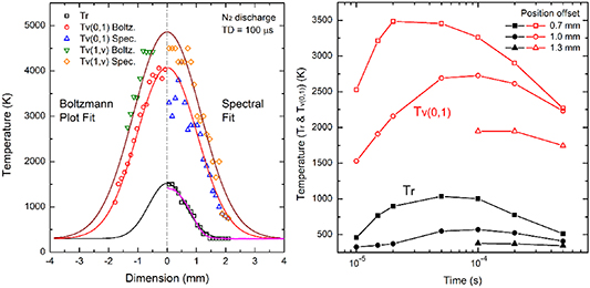
Figure 9. (Left) Spatial distribution of vibrational temperatures ( ,
,  ) and rotational temperature
  at the time delay of 100 µs. (Right) The temporal evolution of rotational and vibrational temperatures at different positions offset from the center of the plasma region.
Download figure:
Standard image High-resolution imageThe N2 nanosecond pulse discharge provides the unique non-equilibrium gas environment with rapid energy exchange among the internal modes. Figure 9 (on the right) shows the temporal evolution of the vibrational temperature  and the rotational temperature
  in the discharge afterglow at different locations. Near the center of the plasma afterglow (i.e. 0.7 mm offset), the vibrational temperature increases rapidly in the first 20 µs and then gradually decays to a moderate value (2000 K) at 500 µs. The rotational temperature has a smooth rise which reaches the maximum at around 50 µs. After that it decays to 500 K at the time delay of 500 µs. At the outer layer (i.e. 1.0 mm offset), both the vibrational and rotational temperatures have lower values and the later arrival of the maximum (∼100 µs) compared to those in the inner layer, indicating the temporal and spatial evolution of the plasma afterglow. At a 1.3 mm offset, the SRS signal is too week to extract the temperature information at early time delays, which is later detectable until the time delay of 100 µs. Both the vibrational and rotational temperature at this location have the lowest values comparing to the other two cases. We should note that for nitrogen, the V–T transition rate from
  = 1 to
  = 0 is very slow (a few milliseconds in pure N2) [50], so within the time frame of these measurements, the population on
  = 1 state does not decay. The V–V rates can be fast (only an anharmonic energy gap), so the vibrational state relax, typically colliding with
  = 0 and populating
  = 1 (an endothermic reaction [51]), but leading to a locked-in
  = 1 state, so for long times (milliseconds)
  should remain greater than
  and be greater than or equal to
  absent Treanor pumping.
3.3. Gladstone–Dale term and scalar polarizability
In sections 3.1 and 3.2, the refractive index  , rotational temperature
  , and vibrational non-equilibrium state (described by
  and
and  ) have been quantitatively measured by Mach-Zehnder interferometry and spontaneous Raman scattering spectroscopy. Based on these measurements, the scalar dipole polarizability
  can be inferred using the Lorentz–Lorenz relation for dilute gases (equation (3)). The gas number density
  is calculated by the ideal (perfect) gas law
  . We assume that the local pressure has equilibrated to the initial pressure (90 Torr) after the time delay of 10 µs, long enough for the pressure wave propagating out from the plasma afterglow region. The pressure wave is indeed detected in both interferometry and Raman scattering experiments, which has been observed in previous work [52]. It is worth noting that the wave pressure and propagation is the result of the fast isochoric gas heating during the first tens of nanoseconds after the discharge initiation. Based on shockwave studying in previous work [52], the local pressure can be assumed to be the same as the initial pressure value (i.e. 90 Torr) after approximately 10 µs. The spatial distribution of the Gladstone-Dale term
  at different time delays ranging from 10 to 500 µs, shown in figure 10(a), has been calculated based on the refractive index and gas temperature measurements. Specifically, the spatial-resolved experimental data of rotational temperature and refractive index are curve fitted by analytical equations as shown in figures 10(b) and (c) at the time delay of 10 µs. Therefore, the Gladstone-Dale terms in figure 10(a) are all analytically presented. According to equation (3), the scalar polarizability is then obtained as the function of
  ,
,  , as presented in figure 11.

Figure 10. (a) The spatial distribution of the Gladstone–Dale term at different time delays after the start of discharge pulse. (b) The spatial distribution of the rotational temperature  at the time delay of 100 µs. (c) The spatial distribution of the phase delay and refractive index (
 −1) at the time delay of 100 µs.
Download figure:
Standard image High-resolution image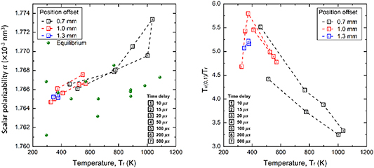
Figure 11. (Left) The scalar polarizability distribution as a function of the rotational temperature; (right) the temperature ratio between vibrational  and rotational temperature
  as a function of the rotational temperature.
Download figure:
Standard image High-resolution imageFigure 11 (on the left) shows the scalar polarizability as a function of rotation temperature for delay times and locations inside the plasma afterglow. Specifically, near the center of the plasma region (0.7 mm offset), the scalar polarizability has a significant increase with the increase of rotational temperature, reaching the maximum at the time delay of 50 µs. After that it decays along with the temperature decrease. For the outer layer cases (1.0 and 1.3 mm offsets), the scalar polarizability does not have a significant increase with a relatively low rotational temperature. Compared to the equilibrium results, the scalar polarizability has a slight but significant increase (4  10−6 nm3) under the non-equilibrium conditions. Figure 11 (on the right) shows the temporal evolution of the ratio between
  and
and  . In the entire plasma afterglow region,
  is much greater than
  (at least a factor of 3). Near the center plasma afterglow region (0.7 mm offset), the ratio between
  and
and  is first rapidly decreasing in the first 50 µs, which is due to the quicker
  increase compared to
  . After that (
 100 µs), the ratio has a moderate increase due to the slow V-T transition rate from
  = 1 to
  = 0. At the outer layers (1.0 and 1.3 mm offsets), high ratio values are present with a lower rotational temperature. No strong dependence of scalar polarizability on the variations of the non-equilibrium is observed with a low rotational temperature. These are the first direct measurements, to the authors' knowledge, of both the rotational temperature and non-equilibrium dependence of the scalar polarizability.
3.4. Semi-classical model and simulation results
In previous work, we theoretically studied the vibrational non-equilibrium effects on scalar polarizability in molecular nitrogen and oxygen [13]. The molecular polarizability calculations have been performed based on a semi-classical model, which is briefly introduced here. The polarizability is calculated considering the virtual transitions from the ground electronic manifold to upper levels (i.e. vibrational, rotational, and continuum states),
with the total polarizability is given as
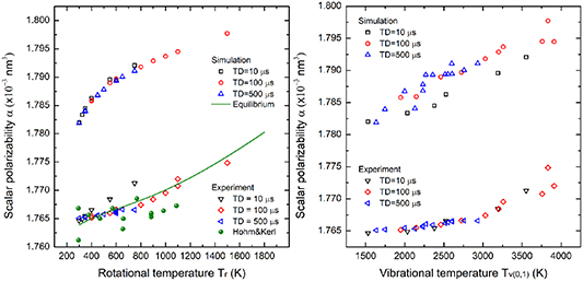
In thermal equilibrium, the population fractions follow a Boltzmann distribution, however, for non-equilibrium processes, they can substantially depart from this distribution. We take this effect into account by assuming that the vibrational and the rotational populations are separately thermalized with different temperatures. Based on the experimental data of Hohm and Kerl showing a slight dependence of polarizability on temperature, we chose as a fundamental set oscillator strengths from the paper [53]. Results of calculations of polarizability for equilibrium and for the non-equilibrium cases shown in figure 12 using measured rotational and vibrational temperatures as the input parameters. Figure 12 (on the left) shows the simulation results for non-equilibrium at three different time delays as a function of the measured rotational temperature, and figure 12 (on the right) shows the simulation results plotted as a function of the measured vibrational temperature. The shift of the scalar polarizability from the thermal equilibrium calculation to the non-equilibrium states (i.e. 10, 100, and 500 µs) is around 1% due to the vibrational non-equilibrium population in the discharge afterglow, however, such a shift was not detected in the experiment. Figure 12 on the right shows the calculated scalar polarizability monotonically increasing with the vibrational temperature (∼0.33% per 1000 K). The scattering distribution of data is due to the measurement uncertainty of the rotational temperature aforementioned in section 3.2. Overall, the calculation predicted higher values of polarizability for the non-equilibrium case with the difference around 1% between calculation and experimental results, although the trends with increasing rotational and vibrational temperatures are qualitatively captured. Continuing efforts are aimed at understanding the ∼1.8  10−5 nm3 offset between the model and experimental results in the low vibrational temperature regime.
Figure 12. (Left) The calculated scalar polarizability values as the function of the rotational temperature and (right) the vibrational temperature versus experimental results.
Download figure:
Standard image High-resolution image
4. Conclusion
In this study, we report refractive index and scalar polarizability measurements under non-equilibrium conditions which are created by a high-voltage nanosecond pulsed discharge at a pressure of 90 Torr. Refractive index, rotational temperature, and vibrational temperature have been measured in the discharge afterglow with the time delay ranging from 10 to 500 µs. The pressure is assumed to be equilibrated (i.e. 90 Torr) after the pressure wave propagates out from the testing region after 10 µs. Mach–Zehnder interferometry is employed to measure the optical phase delay ( ) and obtain the spatially-resolved refractive index profile, while spontaneous Raman scattering spectroscopy is used to characterize the conditions of the discharge afterglow at the same time delays. From this extensive data set, the Gladstone–Dale term and the scalar polarizability have been calculated with measured refractive index
  and gas density
  according to the Lorentz–Lorenz relation. To our acknowledge, it is the first time that the Gladstone–Dale term and scalar polarizability have been measured in a non-equilibrium gas with a wide rotational temperature range (i.e. 300–1000 K). The semi-classic model has been employed to calculate the mean polarizability with the experimental results as input parameters. The model prediction that the slope of polarizability increases depending on rotational and vibrational temperature has shown reasonably good agreement with the experimental results.
Acknowledgments
This work has been supported by internal funds of Texas A&M University and by the Air Force Research Laboratory through the Ohio Aerospace Institute under Subcontract OAI-C2644-18012.