Sparse Logistic Regression With L1/2 Penalty for Emotion Recognition in Electroencephalography Classification
 Dong-Wei Chen1
  Yong Liang
 Lan Huang
- 1School of Electronic Information Engineering, University of Electronic Science and Technology of China, Zhongshan, China
- 2Faculty of Information Technology, Macau University of Science and Technology, Macau, China
- 3State Key Laboratory of Quality Research in Chinese Medicines, Macau University of Science and Technology, Macau, China
Emotion recognition based on electroencephalography (EEG) signals is a current focus in brain-computer interface research. However, the classification of EEG is difficult owing to large amounts of data and high levels of noise. Therefore, it is important to determine how to effectively extract features that include important information. Regularization, one of the effective methods for EEG signal processing, can effectively extract important features from the signal and has potential applications in EEG emotion recognition. Currently, the most popular regularization technique is Lasso (L1) and Ridge Regression (L2). In recent years, researchers have proposed many other regularization terms. In theory, Lq-type regularization has a lower q value, which means that it can be used to find solutions with better sparsity. L1/2 regularization is of Lq type (0 < q < 1) and has been shown to have many attractive properties. In this work, we studied the L1/2 penalty in sparse logistic regression for three-classification EEG emotion recognition, and used a coordinate descent algorithm and a univariate semi-threshold operator to implement L1/2 penalty logistic regression. The experimental results on simulation and real data demonstrate that our proposed method is better than other existing regularization methods. Sparse logistic regression with L1/2 penalty achieves higher classification accuracy than the conventional L1, Ridge Regression, and Elastic Net regularization methods, using fewer but more informative EEG signals. This is very important for high-dimensional small-sample EEG data and can help researchers to reduce computational complexity and improve computational accuracy. Therefore, we propose that sparse logistic regression with the L1/2 penalty is an effective technique for emotion recognition in practical classification problems.
1. Introduction
Electroencephalography (EEG) is a means of obtaining data through sensors (Rashid et al., 2018; Uktveris and Jusas, 2018). The brain-computer interface (BCI), also known as a direct neural interface, is an interdisciplinary cutting-edge technology that represents a direct link between human or animal brains (or brain cell cultures) and external devices (Wolpaw et al., 2000, 2002; Cecotti, 2011; Chaudhary et al., 2016; Ramadan and Vasilakos, 2017). The role of BCI is to establish communication between the human brain and external computers or other intelligent electronic devices (Jin et al., 2015; Li et al., 2016). Emotional cognition is a very important part of BCI. Emotional recognition generally refers to the use of an individual's physiological or non-physiological signals to automatically identify their emotional state (Cowie et al., 2001; Busso et al., 2004). Emotional recognition is an important part of emotional computing and is of great importance in medicine and engineering.
Pattern recognition is a crucial step in accurately classifying or decoding EEG signals in BCI. How to effectively identify and classify EEG features is still the subject of research. Several EEG classification algorithms have been proposed, including logistic regression, support vector machine (Chen et al., 2019), decision tree (Subasi and Erçelebi, 2005; Polat and Güneş, 2007; Subasi and Gursoy, 2010), and convolutional neural networks (Baran-Baloglu et al., 2019; Bernal et al., 2019). These methods tend to focus on classification, and usually aim to directly find a possible classification model. The classification process does not usually involve sparse processing. However, EEG data tend to be characterized by high dimensions and small sample sizes. Therefore, these methods are prone to over-fitting or low precision. There are two main approaches to this problem. The first is dimension reduction, the main examples of which are the PCA and LDA methods (Subasi and Gursoy, 2010). These methods use matrix decomposition to map the original N-dimensional features into K dimensions, thereby changing the original values of the data. The second approach is regularization, currently represented by the L0, Lasso (L1), Ridge Regression, and Elastic Net methods (Silva et al., 2004; Zou and Hastie, 2005; Friston et al., 2008; Wang et al., 2015). In theory, the L0 penalty is the best in the case of sparseness, but this method involves an NP-hard problem (Schölkopf and Smola, 2001). Therefore, the Lasso (L1) penalty is most often used. The L1 penalty is the sum of the absolute values of the elements in the weight vector w, usually expressed as ||ω||1 (Tibshirani, 1996). The Ridge Regression is the sum of the squares of the elements in the weight vector w and the square root, usually expressed as ||ω||2 (Ng, 2004). The Elastic Net method was proposed to overcome the respective limitations of L1 and Ridge Regression. This method combines the L1 penalty and Ridge Regression to achieve a better effect. Recently, in order to obtain a sparser and more solvable penalty term, Xu proposed a new L1/2 penalty and applied it to signal recovery problem (Xu et al., 2012); the result of the this penalty is more sparse than that of the L1 penalty and can be solved. It is thus preferable in theory (Xu et al., 2010).
In the field of multi-category EEG emotion recognition, sparse logistic regression models based on regularization have achieved excellent results in EEG signal emotion recognition in recent years. For example, Ryali et al. (2010) proposed a novel method based on logistic regression using a combination of L1 and Ridge Regression that could more accurately discriminate brain regions across multiple conditions or groups (Ryali et al., 2010). Hussein et al. (2018) proposed a feature learning method based on L1-penalized robust regression, which could recognize the most prominent features pertinent to epileptic seizures in EEG spectra (Hussein et al., 2018). Conroy and Sajda (2012) used Ridge Regression to improve EEG classification results (Conroy and Sajda, 2012). Inspired by the above methods, we studied sparse logistic regression models with the L1/2 penalty, with a particular focus on applications in EEG sentiment classification. The L1/2 penalty can be penalized as representatives of (0 < q < 1) and has many attractive features, such as unbiasedness, sparsity, and oracle attributes (Xu et al., 2010). Current logistic regression models using the L1/2 penalty have achieved excellent results in biological fields, such as genetic screening (Liang et al., 2013; Liu et al., 2014; Huang et al., 2016).
In this work, we develop a coordinate reduction algorithm for L1/2 regularization in a sparse logistic regression framework and build a three-classification sparse regularization logistic regression model for EEG sentiment data (Figure 1). This method is suitable for use with large EEG datasets with a low sample size. Tests were performed using a simulation dataset and a real dataset (SEED and DEAP). An experimental comparison with sparse logistic regression using the L1 penalty, Ridge Regression, and Elastic Net penalty points was used to validate the L1/2 penalty logistic regression method proposed in this paper.

Figure 1. Flow chart of sparse logistic regression based on L1/2 penalty. First, we divide a three-category dataset (such as SEED) into three two-category datasets (the upper part). Next, the green part represents training a classifier based on L1/2 penalty logistic regression for each binary classification dataset. Each classifier will reduce the sample dimension from N to M after sparsification. For each input EEG data, we will get three binary classification results. Through summary analysis, the final three classification results are obtained.
2. Materials and Methods
2.1. Materials
2.1.1. Simulation Dataset
We used the Python method sklearn.dataset.make_classification to generate a random simulation three-classification dataset, with a sample number of 1,200 and a characteristic of 1,000. Each class is composed of a number of gaussian clusters each located around the vertices of a hypercube in a subspace of dimension 3. For each cluster, informative features are drawn independently from N(0, 1) (Equation 1) and then randomly linearly combined within each cluster in order to add covariance. The clusters are then placed on the vertices of the hypercube. And we added useless features drawn at random to this dataset use parameters n_redundant = 2 and n_repeated = 2 to add two redundant features to the information feature and repeated it twice. We selected 80% of the samples as the training dataset and used the remaining 20% as the verification dataset.
2.1.2. SEED Dataset
Experiments were conducted using a public emotion EEG dataset called SEED, which uses film fragments as emotion-inducing materials and includes three categories of emotion: positive, neutral, and negative. In each experiment, the participants will watch movie clips of different emotional states. Each clip will be played for about 4 min. In the experiment, three types of movie clips will be played. Each type of movie clips contains five movies, and in total 15 movies. These movie clips are all from Chinese movies. There is a 5 s prompt before each short film is shown, with 45 s of feedback time after playback, and 15 s of rest after watching. A total of 15 subjects (seven males, eight females, mean age 23.27 years old, the standard deviation of 2.37) participated in the experiment, and all subjects had normal visual, auditory, and emotional states. The EEG signal, while the subject was watching the movie, was recorded through the electrode cap and the sampling frequency was 1,000 Hz. The experiment used the international 10–20 system and a 62-channel electrode cap. Each volunteer participated in three experiments, and each experiment was separated by about 1 week. Therefore, a total of 15 × 15 × 3 = 675 data samples is formed. Then 200 Hz down-sampling and a bandpass frequency filter from 0 to 75 Hz was applied to obtain a preprocessed EEG dataset. For more information on this dataset, please refer to the website http://bcmi.sjtu.edu.cn/~seed/index.html. Before using this dataset, we used the PCA method to preprocess the data and to reduce the dimension from 11,470 to 528 in the beta band, and from 57350 to 528 in the combined band (keep 95% variance information), in order to reduce the computational complexity and time complexity (according to the results of running the PCA model based on the SEED dataset, the variance ratio of the first PC is only 30.1%, the variance ratio of the second PC is 9.2%, the variance ratio of the third PC is only 4.9%, and the sum of the variance ratios of the three largest contributing PCs is only 44.2%, which is much <95% variance ratio required in this paper. In this situation, program results show that we need 528 PCs to achieve a 95% variance ratio).
2.1.2.1. Beta band dataset
The SEED EEG dataset contained five EEG bands. The main frequency range of the five bands was 14–30 Hz. The frequency range of the beta brain wave is 14–30 Hz. When the brain is in a conscious condition, the mind is in a state of tension, and the individual is very sensitive to their surroundings, so the energy intensity of the beta wave will be higher than the others. The attention is focused on the external environment in a scattered manner, and the brain is prone to fatigue. Most people are in this state during the day. Previous studies have shown that the main role of the beta band is to reflect emotions and cognition (Ahmed and Basori, 2013; Jabbic et al., 2015). Therefore, we chose beta brain waves for experimental analysis. The beta brain wave frequency band of the SEED dataset contained 660 samples.
2.1.2.2. Combined band dataset
In order to verify the performance of our method, we also tested it using the EEG dataset for the total frequency band. The EEG signal is decomposed into five frequency bands according to EEG rhythm, comprising delta (1–3 Hz), theta (4–7 Hz), alpha (8–13 Hz), beta (14–30 Hz), and gamma (31–50 Hz) bands. These five frequency band signals were combined to form a new combined frequency band dataset (Lin et al., 2010; Nie et al., 2011). Therefore, six EEG datasets representing different frequency bands were obtained. Finally, four classification methods, namely sparse logistic regression with L1/2 penalty, sparse logistic regression with L1 penalty, Ridge Regression, and Elastic Net, were tested and verified using the above datasets. In the experiments, 660 samples were randomly assigned to the mutually exclusive training set (80%) and the remainder formed the verification set (20%).
2.1.3. DEAP Dataset
The dataset named DEAPA Database for Emotion Analysis Using Physiological Signals (Koelstra et al., 2012) can be found at the website http://www.eecs.qmul.ac.uk/mmv/datasets/deap/. The DEAP dataset consists of two parts; first the ratings from an online self-assessment where 120 1-min extracts of music videos were each rated by 14–16 volunteers based on arousal, valence and dominance; second, the participant ratings, physiological recordings and face video of an experiment where 32 volunteers watched a subset of 40 of the above music videos. EEG and physiological signals were recorded, and each participant also rated the videos as above. For 22 participants frontal face video was also recorded. At the end of each video, participants are required to fill out a self-assessment (SAM) form to score from 1 to 9. Arousal ranges from inactive (1) to active (9). Valence ranges from unpleasant (1) to pleasant (9). The rating range of liking and dominance is also between 1 and 9, which means helpless and a weak feeling (1) to an empowered feeling (9). The DEAP dataset includes 32-channel EEG signals, and peripheral physiological signals, such as GSR signals, EOG signals, EMG signals, PPG signals, Temp, and Status. All data was down-sampled to 128 Hz, where the EEG signal data became a 60 s test signal and a 3 s baseline. A zero-phase bandpass filter of 4–45 Hz was applied. In this paper, the 32-channel EEG was divided into two classes according to arousal, Positive (more than 6) and Negative (Low 4). For the DEAP dataset, we only used data from combined frequency bands for experiments.
2.1.4. Cross-Validation
To ensure the accuracy of the results, a 5-fold cross-validation method was used in all the experiments. The 5-fold cross-validation first divides all the data into five sub-samples. One of the sub-samples is repeatedly selected as the test set, and the other four samples are used for training, repeated five times in total and the average of five times and its error range is selected. In addition to using 5-fold cross-validation, all experiments in this paper also performed 100 repeated experiments to obtain its averages and errors.
2.2. Methods
This paper constructs a three-category L1/2 penalty logistic regression method. The main focus of this work was the general ternary classification problem. A ternary classifier was built, consisting of three small two classifiers, each of which was identical in construction. This model produced three two-classifier results, which could be summarized to give the ternary classification output, as shown in Figure 1. We first summarize a three-category dataset into three two-category datasets, and then establish three two-category L1/2 penalty logistic regression methods. According to the results of each two-classifier, the final three-classification result is obtained. The construction method of the L1/2 penalty logistic regression method for the two classifications is as follows.
2.2.1. Sparse Logistic Regression With L1/2 Penalty
Here, we describe the construction of a sparse two-class logistic regression method based on the L1/2 penalty. Suppose we have n samples, where D = (X1, y1), (X2, y2), ..., (Xn, yn), Xi = (xi1, xi2, ..., xip) is the ith input mode, and the dimension is p; yi is the corresponding variable, with a value of 0 or 1: yi = 0 represents the ith sample in category 1, and yi = 1 represents the ith sample in category 2. Vector Xi includes the p features of the ith samples (for all p EEG signals), and xij represents the EEG signal value of j in the ith sample. Defining the classifier as f(x) = ex/(1 + ex) allows y to be correctly predicted using the class label y for any input x.
The logistic regression is expressed as:
where β = (β0, β1, ..., βp) is the estimated coefficient, and note is the intercept. The log likelihood is
We obtain β by minimizing the log likelihood. In high-dimensional applications with p >> n, directly solving the logical model given in Equation (3) is ill-posed and may lead to over-fitting. Therefore, it is necessary to apply a regularization method to solve the over-fitting problem. When adding a regularization term to Equation (3), the sparse logistic regression can be modeled as:
where λ > 0 is an adjusting parameter and P(β) is a regularization item. The most popular regularization technique is Lasso (L1) (Tibshirani, 1996), which uses the regularization term P(β) = ∑|β|. In recent years, many Lq-type regularization terms have been proposed, including SCAD (Shailubhai et al., 2000), Elastic Net (Maglietta et al., 2007), and MC+ (Wiese et al., 2007).
In theory, Lq-type regularization P(β) = ∑|β|q with a lower q value will result in a better solution with more sparsity, such as signal recovery problem and genetic selection (Xu et al., 2010, 2012; Liang et al., 2013). However, when q is very close to zero, convergence may be difficult. Therefore, Xu et al. (2010) further explored the nature of Lq(0 < q < 1) regularization and revealed the importance and effects of L1/2 regularization. They proposed that when , L1/2 regularization produces the most sparse results, with relatively easy convergence compared with L1 regularization. At , there is no significant difference in the performance of the Lq penalty. Furthermore, solving L1/2 normalization is much simpler than solving L0 normalization. Therefore, L1/2 regularization can be used as a representative of Lq(0 < q < 1) regularization. In this paper, we apply the L1/2 penalty to the logistic regression model. A sparse logistic regression model based on the L1/2 penalty has the following form:
L1/2 regularization has been shown to have many attractive features, including unbiasedness, sparsity, and oracle features (Xu et al., 2010, 2012; Liang et al., 2013). Theoretical and experimental analyses show that regularization is a competitive approach. Our work in this paper also reveals the effectiveness of L1/2 regularization in solving non-linear logistic regression problems with a small number of predictive features (EEG signals).
2.2.2. Coordinated Descent Algorithm for L1/2 Penalty Logistic Regression
The coordinate descent algorithm (Friedman et al., 2007, 2010) is a “single-at-time” method. Its basic steps can be described as follows: for each coefficient, the remaining elements are partially fixed relative to the optimization objective function βj(j = 1, 2, ..., p) in the nearest updated value.
Before introducing the coordinate reduction algorithm for non-linear logistic regularization, we first consider the linear regularization case. Assuming that dataset D has n samples, D = (X1, y1), (X2, y2), ..., (Xn, yn), where Xi = (xi1, xi2, ..., xip) is the ith input variable, the dimension is p, and yi is the corresponding response variable. Variables are standardized: and . Therefore, the linear regression of the regularization term can be expressed as:
where P(β) is the regularization term. The coordinate descent algorithm can be used to solve βj, and the other βk≠j (k ≠ j represents the parameters that remain after jth the element is removed) are fixed. According to the idea of coordinate descent algorithm, only one variable is optimized at each time and other variables are fixed. The function can be expressed as
The first derivative βj can be estimated as:
Defining as the partial residual for fittingβj and , the univariate soft thresholding operator of the coordinate descent algorithm (Busso et al., 2004) for L1 regularization (Lasso) can be defined as:
Similarly, for L0 regularization, the threshold operator of the coordinate descent algorithm can be defined as:
where I is the indicator function. This formula is equivalent to the hard thresholding operator (Silva et al., 2004).
According to Equations (9) and (10), different penalties are associated with different threshold operators. Therefore, Xu et al. (2012) proposed a semi-threshold operator to solve the L1/2 regularization of linear regression models, using an iterative algorithm that can be considered a multivariate half-threshold method. In this paper, we present a univariate half-threshold operator for the coordinate reduction algorithm for L1/2 regularization. Based on Equation (8), the gradient of L1/2 regularization at βj can be expressed as:
where βj > 0 and . When βj > 0, the equation (11) can be redefined as:
A univariate half-threshold operator can be expressed as:
where ϕλ(ω) satisfies:
The L1/2 regularized coordinate reduction algorithm reuses the univariate half-threshold operator. This coordinate descent algorithm for regularization can be extended to sparse logistic regression models. Based on the objective function of sparse logistic regression (Equation 4), a Taylor series expansion of l(β) has the following formula:
where is an estimated response, is a weight, and is a value evaluated using the current parameters. Redefining the partial residual for fitting the current as:
we can directly apply the coordinate descent algorithm with the L1/2 penalty for sparse logistic regression.
3. Results
Sparse logistic regression with the L1/2, L1 penalties, and Ridge Regression and the Elastic Net method were tested using the simulated dataset and the real dataset. Four evaluation methods were used to evaluate the performance of the proposed model. A confusion matrix was used to compare the results between the various methods. This is a situation analysis table that summarizes the prediction results of a classification model in machine learning. The records in the dataset are summarized in matrix form according to the real category and the classification criteria predicted by the classification model. The rows of the matrix represent the true values, and the columns represent the predicted values. The computational accuracy of the proposed method was also used as a measure of quality, where the accuracy is defined as the ratio of the number of samples correctly classified by the classifier to the total number of samples in the test dataset. However, accuracy is not always effective for performance evaluation, especially if the number of samples with different labels are not exactly equal. Therefore, we also analyzed precision and recall for further comparison of the three two-classifiers. Here, precision refers to the proportion of all predicted true positives in positive classes, and recall refers to the proportion of positives found in all positive classes. All experiments used 5-fold cross-validation to ensure the stability of the proposed model.
3.1. Analysis of Simulation Dataset
We used sparse logistic regression with the L1/2, L1 penalties, and Ridge Regression and Elastic Net for experiments and comparisons. Table 1 shows the accuracy and recall results for the three categories and four methods using the simulation dataset.

Table 1. Precision and recall results for sparse logistic regression with L1/2 and L1 penalties, Ridge Regression and Elastic Net.
As shown in Table 1, in terms of precision, the sparse logistic regression method with the L1/2 penalty proposed in this paper was superior to the other methods in all three categories. For neutral emotion, the precision of the proposed method was 100%, which was 2, 2, and 8% higher than those of the Elastic Net method, sparse logistic regression with L1 penalty, and Ridge Regression, respectively. For positive emotion, the precision of the proposed method was 99%, which was 5, 2, and 15% higher than those of the Elastic Net method, sparse logistic regression with L1 penalty, and Ridge Regression, respectively. For negative emotion, the precision of the proposed method was 100%, which was 2, 2, and 37% higher than those of the Elastic Net method, sparse logistic regression with L1 penalty, and Ridge Regression, respectively. In terms of recall rate and precision rate, the results for sparse logistic regression with L1/2 penalty were better than those of the other three methods for positive emotion, negative emotion, and neutral emotion. For neutral emotion, the recall rate of the proposed method was 100%, which was 1, 1, and 16% higher than those of the Elastic Net method, sparse logistic regression with L1 penalty, and Ridge Regression, respectively. For positive emotion, the recall rate of the proposed method was 100%, which was 15% higher than that of the sparse logistic regression method with Ridge Regression, and the same as those of the Elastic Net method and sparse logistic regression with L1 penalty. For negative emotion, the recall rate of the proposed method was 98%, which was 10, 6, and 29% higher than those of the Elastic Net method, sparse logistic regression with L1 penalty, and Ridge Regression, respectively. Overall, the experimental results show that sparse logistic regression with the L1/2 penalty is superior to the three existing regularization methods.
Figure 2 shows the confusion matrix for generating prediction results using sparse logistic regression with the L1/2 and L1 penalties for simulation datasets. As shown in Figure 2, the accuracy of the sparse logistic regression method with L1/2 penalty was 99.6%, and The results of the proposed method were significantly better than those obtained using sparse logistic regression with L1 penalty or Ridge Regression, or the Elastic Net method (Supplementary Figure 1). In the simulated dataset, there is only one label that was predicted incorrectly, using the sparse logistic regression method with L1/2 penalty. However, there are six labels that were predicted incorrectly using the sparse logistic regression method with L1 penalty. Thus, sparse logistic regression with the L1/2 penalty had the highest classification accuracy and the best effects, indicating the superiority of this method in terms of accuracy for the classification of datasets. Next, we tested our method using a real EEG emotion dataset.
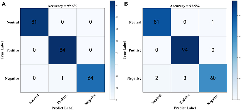
Figure 2. The confusion matrix using simulation dataset. (A) Confusion matrix for generating prediction results using sparse logistic regression with L1/2 penalty, (B) Confusion matrix for generating prediction results using sparse logistic regression with L1 penalty.
3.2. Analysis of Beta Band Dataset
Sparse logistic regression with the L1/2, L1 penalties, and Ridge Regression and Elastic Net were used for all experiments and comparisons. Table 2 shows the accuracy and recall for the three categories using the four methods for this dataset.
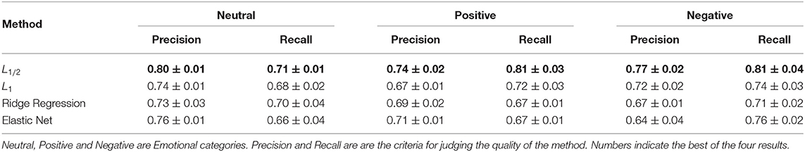
Table 2. Precision and recall results for sparse logistic regression with L1/2 and L1 penalties, Ridge Regression and Elastic Net for the beta band dataset.
As shown in Table 2, in terms of precision, the sparse logistic regression method with L1/2 penalty proposed in this paper was superior to other methods in all three categories. For neutral emotion, the precision of the proposed method was 80%, which was 4, 6, and 7% higher than those of the Elastic Net method, and sparse logistic regression with L1 penalty and Ridge Regression, respectively. For positive emotion, the precision of the proposed method was 74%, which was 3, 7, and 5% higher than those of the Elastic Net method, and sparse logistic regression with L1 penalty and Ridge Regression, respectively. For negative emotion, the precision of the proposed method was 77%, which was 13, 5, and 10% higher than those of the Elastic Net method, and sparse logistic regression with L1 penalty and Ridge Regression, respectively. In terms of recall rate and precision rate, the results of the sparse logistic regression method with L1/2 penalty were better than those of the other three methods for positive emotion, negative emotion, and category 3. For neutral emotion, the recall rate of the proposed method was 70%, which was 4 and 2% higher than those of Elastic Net method and sparse logistic regression with L1 penalty, respectively, and the same as that of Ridge Regression. For positive emotion, the recall rate of the proposed method was 81%, which was 14, 9, and 14% higher than those of the Elastic Net method, and sparse logistic regression with L1 penalty and Ridge Regression, respectively. For negative emotion, the recall rate of the proposed method was 81%, which was 5, 7, and 10% higher than those of the Elastic Net method, and sparse logistic regression with L1 penalty and Ridge Regression, respectively. Overall, the experimental results show that the sparse logistic regression method with L1/2 penalty is superior to the three existing regularization methods.
Supplementary Figure 2 shows an accuracy box plot for the different methods obtained using 5-fold cross-validation. It can be seen from the box plot that the results for the sparse logistic regression method with L1/2 penalty were significantly better than those of the other three methods.
Figure 3 shows the confusion matrix for generating prediction results using sparse logistic regression with the L1/2 and L1 penalties for the two datasets. As shown in Figure 3, the accuracy of sparse logistic regression with L1/2 penalty was 77.3%, and the results obtained with the proposed method were significantly better than those for sparse logistic regression with the L1 penalty or Ridge Regression or the Elastic Net method (Supplementary Figure 3). In the SEED Beta band dataset, there were 30 labels that were predicted incorrectly using the sparse logistic regression method with L1/2 penalty with the main errors concentrated in the Neutrals class. However, compared with the sparse logistic regression method with L1/2 penalty, the number of incorrect labels is 5 fewer. It can be concluded that sparse logistic regression with the L1/2 penalty has the highest classification accuracy and the best effects, indicating that this method is more accurate for the classification of datasets.
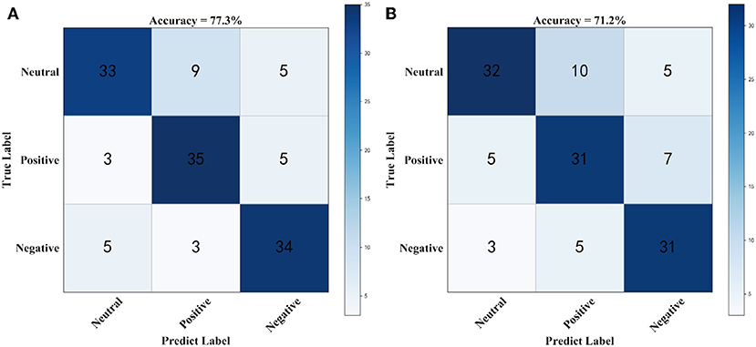
Figure 3. The confusion matrix using beta band dataset. (A) Confusion matrix for generating prediction results using sparse logistic regression with L1/2 penalty, (B) Confusion matrix for generating prediction results using sparse logistic regression with L1 penalty.
In order to verify the sparsity of the L1/2 penalty logistic regression in EEG sentiment dataset. This paper counts the number of data points retained after different Sparse methods are run. As can be seen from the Table 3, in the SEED-band data set, the L1/2 penalty retains the least number of points. In the three binary classifiers, only 125 data points are retained, while the L1 method retains 252, 199, and 271 data points, respectively. Ridge regression and Elastic Net retained all data points. This verifies that in the EEG sentiment dataset, the L1/2 penalty used in this paper has the best sparsity.
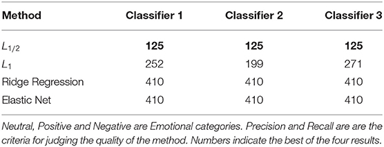
Table 3. The results of Number of points retained after sparsification by the sparse Logistic regressions with L1/2, L1 penalties, Ridge Regression, and Elastic Net in beta band dataset.
3.3. Analysis of Combined Band Dataset
As shown in Table 4, in terms of precision, the sparse logistic regression method with L1/2 penalty proposed in this paper was superior to the other methods in all three categories. For neutral emotion, the precision of the proposed method was 85%, which was 4, 3, and 2% higher than those of the Elastic Net method, sparse logistic regression with L1 penalty, and Ridge Regression, respectively. For positive emotion, the precision of the proposed method was 90%, which was 2% higher than that of sparse logistic regression with L1 penalty or Ridge Regression, and the same as that of Elastic Net method. For negative emotion, the precision of the proposed method was 86%, which was 8 and 11% higher than those of the Elastic Net method and Ridge Regression, and the same as that of sparse logistic regression with L1 penalty. In terms of recall rate and accuracy rate, the results of the sparse logistic regression method with L1/2 penalty were better than those of the other three methods for positive emotion, negative emotion, and category 3. For neutral emotion, the recall rate of the proposed method was 87%, which was 2 and 4% higher than those of the Elastic Net method and sparse logistic regression with L1 penalty, respectively, and the same as that of Ridge Regression. For positive emotion, the recall rate of the proposed method was 88%, which was 7% higher than that of the Elastic Net method, and the same as those of the sparse logistic regression methods with L1 penalty and Ridge Regression. The greatest differences between methods were seen in the negative emotion category, where the recall rate of the proposed method was 86%, which was 3, 7, and 7% higher than those of the Elastic Net method, and the sparse logistic regression methods with L1 penalty and Ridge Regression, respectively. The experimental results show that the sparse logistic regression method with L1/2 penalty is superior to the three existing regularization methods.
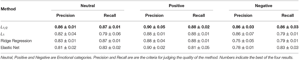
Table 4. Precision and recall results for sparse logistic regression with L1/2 and L1 penalties, Ridge Regression and Elastic Net in the combined band dataset.
Supplementary Figure 4 shows an accuracy box plot for the different methods obtained from the 5-fold cross-validation. It can be seen from the box plot that better results were obtained with sparse logistic regression with the L1/2 penalty than with the L1 penalty or Ridge Regression, or with the Elastic Net method. The fluctuation range for sparse logistic regression with the L1/2 penalty was not large, demonstrating that the proposed method is more stable than the others. Thus, even in the worst case, it is superior to the other methods.
Figure 4 shows the confusion matrix for generating prediction results using sparse logistic regression with the L1/2 and L1 penalties for the two datasets. As shown in Figure 4, the accuracy of the sparse logistic regression method with L1/2 penalty was 87.1%, and the results obtained with the proposed method were significantly better than those for sparse logistic regression with the L1 penalty or Ridge Regression, or the Elastic Net method (Supplementary Figure 5). In the SEED combined band dataset, there are 30 labels that were predicted incorrectly using the sparse logistic regression method with L1/2 penalty with the main errors concentrated in the Negatives class. However, compared with the sparse logistic regression method with L1/2 penalty, the number of incorrect labels is four fewer. Thus, it can be concluded that sparse logistic regression with the L1/2 penalty was the most accurate method for classification of the EEG emotion recognition dataset.
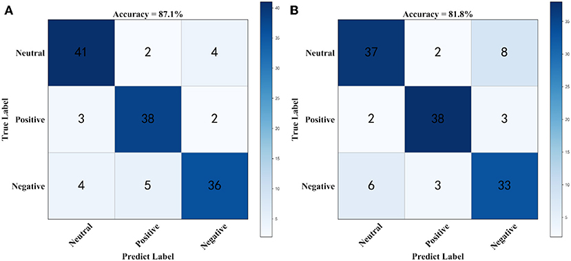
Figure 4. The Confusion matrix using combined band dataset. (A) Confusion matrix for generating prediction results using sparse logistic regression with L1/2 penalty, (B) Confusion matrix for generating prediction results using sparse logistic regression with L1 penalty.
In the SEED-combine dataset, similar conclusions are obtained in this paper. As can be seen from the Table 5, the L1/2 penalty retained only 111, 111, and 140 data points in the three binary classifiers, while the L1 method retained 214, 163, and 22 data points, respectively. Ridge regression and Elastic Net retained all data points. The L1/2 penalty retained the fewest data points but gave the best results. It shows that the L1/2 penalty used in this paper has excellent sparsity in EEG sentiment data.
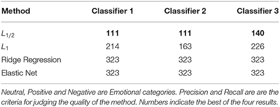
Table 5. The results of Number of points retained after sparsification by the sparse Logistic regressions with L1/2, L1 penalties, Ridge Regression, and Elastic Net in combined band dataset.
3.4. Analysis of DEAP Dataset
As can be seen from Table 6, in the SEED dataset, the logistic regression based on the L1/2 penalty proposed in this paper obtained the best results. In terms of the average accuracy, the result of the logistic regression method based on L1/2 penalty reached 71%. Compared to the Ridge Regression and Elastic Net methods, it has improved by 1%. Compared to L1 penalty, it is increased by 3%. In terms of standard deviation, the logistic regression of L1/2 penalty has the smallest fluctuation, showing excellent stability.
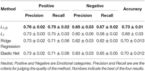
Table 6. The results of accuracy, precision and recall by the sparse Logistic regressions with L1/2, L1 penalties, Ridge Regression, and Elastic Net in DEAP dataset.
Supplementary Figure 6 shows an accuracy box plot for the different methods obtained using 5-fold cross-validation. It can be seen from the box plot that the results for the sparse logistic regression method with L1/2 penalty were significantly better than those of the other three methods.
Table 7 shows the number of loci retained by different methods after calculation. Among them, the L1/2 penalty performed very well, retaining only 301 sites, compared to the 1,537 sites retained by the L1 penalty. The L1/2 penalty retained 80.4% of the sites, but the final result was better than the L1 penalty. Experimental results show that the L1/2 penalty has the best sparsity in the EEG dataset, L1 has poor sparsity, and Ridge Regression and Elastic Net do not have sparsity.
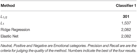
Table 7. The results of Number of points retained after sparsification by the sparse Logistic regressions with L1/2, L1 penalties, Ridge Regression, and Elastic Net in DEAP dataset.
4. Discussion
In EEG sentiment classification, only a small portion of the EEG signal strongly indicates the individual's emotional state. Therefore, feature selection methods play an important role. In this paper, we propose a sparse logistic regression model based on the L1/2 penalty and develop the corresponding coordinate descent algorithm as a new EEG feature selection method. The proposed method uses a new univariate half threshold to update the estimated coefficients. In typical regularization methods, the sparsity of the L0 penalty is theoretically the best; however, this method is difficult to solve, making it less practical. The L1 penalty and Ridge Regression are theoretically mature and are commonly used. However, neither has good enough sparsity. There are regularizers that are sparser than the L1 penalty, such as L1/2 (Xu et al., 2010, 2012). Our results suggest that for EEG emotion datasets, higher sparsity leads to finding features from the EEG signal that are more relevant and have better predictive power for emotion classification.
The L1/2 penalty has been used with very good results in many fields, including image processing and genetic data (Liang et al., 2013; Liu et al., 2014; Huang et al., 2016). This method is very suitable for small-sample, high-dimensional data, such as emotion-based EEG datasets. The existing public datasets typically contain small samples with high dimensions and high levels of noise. If all EEG signals are included in the calculations, the algorithm will have high computational complexity and be prone to overfitting. Therefore, in this work, we used the L1/2 penalty combined with logistic regression and proposed a new three-class sparse logistic regression model. The results demonstrate that the logistic regression method based on the L1/2 penalty performs better than other regularization methods. That is, the sparseness of the L1/2 penalty in the EEG emotional dataset was better than those of the L1 penalty and Ridge Regression. Simulation and real data experiments showed that sparse logistic regression with the L1/2 penalty achieved higher classification accuracy than the conventional L1, Ridge Regression, and Elastic Net regularization methods. Therefore, sparse logistic regression with L1/2 penalty is an effective technique for EEG sentiment classification. To verify the sparsity of the L1/2 penalty logistic regression in EEG sentiment dataset, we count the first five EEG Positions retained by the L1/2 penalty in two datasets (Supplementary Tables 1, 2). Based on data from brainmaster magazine (company) and existing articles (Larsen et al., 2000; Jordan et al., 2001; Lin et al., 2010; Zheng and Lu, 2015). In SEED dataset, all electrode points, including FP1, F8, FPZ, FT8, and FP2 are related to Experiencing/processing emotion. In the DEAP dataset, among them FC5, FC6, CP6, and PO4 Positions are related to Experiencing/processing emotion. The AF3 Position is related to Fear response. Combining the L1/2 penalty in the experiment, yielded the least points of all methods. This shows that the L1/2 penalty has good sparsity for EEG sentiment data. It may also mean that the AF3 Position and EEG processing emotion are highly correlated. In this work, we only combined the L1/2 penalty with the logistic regression method and did not consider combinations including the latest brain networks or deep learning methods (Bernal et al., 2019). Therefore, further work is needed. However, we believe that our proposed approach complements existing sparse methods for EEG emotional data classification well (Wang et al., 2019), which will help researchers to better analyze such data.
Data Availability Statement
Publicly available datasets were analyzed in this study. This data can be found here: http://bcmi.sjtu.edu.cn/~seed/index.html and http://www.eecs.qmul.ac.uk/mmv/datasets/deap/.
Ethics Statement
Written informed consent was obtained from the individual(s) for the publication of any potentially identifiable images or data included in this article.
Author Contributions
D-WC and RM proposed the method. Z-YD conducted the experiments. Y-YL, YL, and LH read and modified the manuscript. All authors contributed to the manuscript and approved the submitted version.
Funding
This research was supported by the Zhongshan City Team Project (Grant No. 180809162197874), the Research Projects for High-Level Talents of University of Electronic Science and Technology of China, Zhongshan (417YKQ8), and the Characteristic Innovation Project of Guangdong Province (2017GXJK217); Guangdong Provincial Department of Education, 2017 Key Scientific Research Platform and Scientific Research Project (2017GCZX007). Project for Innovation Team of Guangdong University (No. 2018KCXTD033).
Conflict of Interest
The authors declare that the research was conducted in the absence of any commercial or financial relationships that could be construed as a potential conflict of interest.
Supplementary Material
The Supplementary Material for this article can be found online at: https://www.frontiersin.org/articles/10.3389/fninf.2020.00029/full#supplementary-material
References
Ahmed, M. A., and Basori, A. H. (2013). The influence of beta signal toward emotion classification for facial expression control through EEG sensors. Proc. Soc. Behav. Sci. 97, 730–736. doi: 10.1016/j.sbspro.2013.10.294
Baran-Baloglu, U., Talo, M., Yildirim, O., SanTan, R., and Acharya, U. R. (2019). Classification of myocardial infarction with multi-lead ECG signals and deep CNN. Pattern Recognit. Lett. 122, 23–30. doi: 10.1016/j.patrec.2019.02.016
Bernal, J., Kushibar, K., Asfaw, S. D., Valverde, S., Oliver, A., Mart, R., et al. (2019). Deep convolutional neural networks for brain image analysis on magnetic resonance imaging: a review. Artif. Intell. Med. 95, 64–81. doi: 10.1016/j.artmed.2018.08.008
Busso, C., Deng, Z., Yildirim, S., Bulut, M., Lee, C. M., Kazemzadeh, A., et al. (2004). “Analysis of emotion recognition using facial expressions, speech and multimodal information,” in Proceedings of the 6th International Conference on Multimodal Interfaces (New York, NY: ACM), 41–50. doi: 10.1145/1027933.1027968
Cecotti, H. (2011). Spelling with non-invasive brain-computer interfaces—current and future trends. J. Physiol. Paris 105, 106–114. doi: 10.1016/j.jphysparis.2011.08.003
Chaudhary, U., Birbaumer, N., and Ramos-Murguialday, A. (2016). Brain–computer interfaces for communication and rehabilitation. Nat. Rev. Neurol. 12, 513–525. doi: 10.1038/nrneurol.2016.113
Chen, D.-W., Miao, R., Yang, W.-Q., Liang, Y., Chen, H.-H., Huang, L., et al. (2019). A Feature extraction method based on differential entropy and linear discriminant analysis for emotion recognition. Sensors 19:1631. doi: 10.3390/s19071631
Conroy, B., and Sajda, P. (2012). “Fast, exact model selection and permutation testing for L2-regularized logistic regression,” in Proceedings of the Fifteenth International Conference on Artificial Intelligence and Statistics (La Palma), 246–254.
Cowie, R., Douglas-Cowie, E., and Tsapatsoulis, N. (2001). Emotion recognition in human-computer interaction. IEEE Signal Process. Mag. 18, 32–80. doi: 10.1109/79.911197
Friedman, J., Hastie, T., Höfling, H., and Tibshirani, R. (2007). Pathwise coordinate optimization. Ann. Appl. Stat. 1, 302–332. doi: 10.1214/07-AOAS131
Friedman, J., Hastie, T., and Tibshirani, R. (2010). Regularization paths for generalized linear models via coordinate descent. J. Stat. Softw. 33:1. doi: 10.18637/jss.v033.i01
Friston, K., Harrison, L., Daunizeau, J., Kiebel, S., Phillips, C., Trujillo-Barreto, N., et al. (2008). Multiple sparse priors for the M/EEG inverse problem. Neuroimage 39, 1104–1120. doi: 10.1016/j.neuroimage.2007.09.048
Huang, H.-H., Liu, X.-Y., and Liang, Y. (2016). Feature selection and cancer classification via sparse logistic regression with the hybrid L1/2+2 regularization. PLoS ONE 11:e0149675. doi: 10.1371/journal.pone.0149675
Hussein, R., Elgendi, M., Wang, Z. J., and Ward, K. R. (2018). Robust detection of epileptic seizures based on L1-penalized robust regression of EEG signals. Expert Syst. Appl. 104, 153–167. doi: 10.1016/j.eswa.2018.03.022
Jabbic, M., Kohn, P. D., Nash, T., Ianni, A., Coutlee, C., Holroyd, T., et al. (2015). Convergent BOLD and beta-band activity in superior temporal sulcus and frontolimbic circuitry underpins human emotion cognition. Cereb. Cortex 25, 1878–1888. doi: 10.1093/cercor/bht427
Jin, J., Sellers, E. W., Zhou, S., Zhang, Y., Wang, X., and Cichocki, A. (2015). A P300 brain–computer interface based on a modification of the mismatch negativity paradigm. Int. J. Neural Syst. 25, 1550011–1550012. doi: 10.1142/S0129065715500112
Jordan, K., Heinze, H. J., Lutz, K., Kanowski, M., and Jäncke, L. (2001). Cortical activations during the mental rotation of different visual objects. Neuroimage 13, 143–152. doi: 10.1006/nimg.2000.0677
Koelstra, S., Mühl, C., Soleymani, M., Lee, J.-S., Yazdani, A., Ebrahimi, T., et al. (2012). DEAP: a database for emotion analysis; using physiological signals. IEEE Trans. Affect. Comput. 3, 18–31. doi: 10.1109/T-AFFC.2011.15
Larsen, A., Bundesen, C., Kyllingsbk, S., Paulson, O. B., and Law, I. (2000). Brain activation during mental transformation of size. J. Cogn. Neurosci. 12, 763–774. doi: 10.1162/089892900562589
Li, Y., Pan, J., Long, J., Yu, T., Wang, F., Yu, Z., et al. (2016). Multimodal BCIs: target detection, multidimensional control, and awareness evaluation in patients with disorder of consciousness. Proc. IEEE 104, 332–352. doi: 10.1109/JPROC.2015.2469106
Liang, Y., Liu, C., Luan, X.-Z., Leung, K.-S., Chan, T.-M., Xu, Z.-B., et al. (2013). Sparse logistic regression with a L1/2 penalty for gene selection in cancer classification. BMC Bioinformatics 14:198. doi: 10.1186/1471-2105-14-198
Lin, Y.-P., Wang, C.-H., Jung, T.-P., Wu, T.-L., Jeng, S.-K., Duan, J.-R., et al. (2010). EEG-based emotion recognition in music listening. IEEE Trans. Biomed. Eng. 57, 1798–1806. doi: 10.1109/TBME.2010.2048568
Liu, C., Liang, Y., Luan, X.-Z., Leung, K.-S., Chan, T.-M., Xu, Z.-B., et al. (2014). The L1/2 regularization method for variable selection in the Cox model. Appl. Soft Comput. 14, 498–503. doi: 10.1016/j.asoc.2013.09.006
Maglietta, R., D'Addabbo, A., Piepoli, A., Perri, F., Liuni, S., Pesole, G., et al. (2007). Selection of relevant genes in cancer diagnosis based on their prediction accuracy. Artif. Intell. Med. 40, 29–44. doi: 10.1016/j.artmed.2006.06.002
Ng, A. Y. (2004). “Feature selection, L1 vs. L2 regularization, and rotational invariance,” in Proceedings of the 21st International Conference on Machine Learning (ACM), 78. doi: 10.1145/1015330.1015435
Nie, D., Wang, X.-W., Shi, L.-C., and Lu, B.-L. (2011). “EEG-based emotion recognition during watching movies,” in 2011 5th International IEEE/EMBS Conference on Neural Engineering, 667–670. doi: 10.1109/NER.2011.5910636
Polat, K., and Güneş, S. (2007). Classification of epileptiform EEG using a hybrid system based on decision tree classifier and fast Fourier transform. Appl. Math. Comput. 187, 1017–1026. doi: 10.1016/j.amc.2006.09.022
Ramadan, R., and Vasilakos, A. (2017). Brain computer interface: control signals review. Neurocomputing 223, 26–44. doi: 10.1016/j.neucom.2016.10.024
Rashid, U., Niazi, I. K., and Signal, N. (2018). An EEG experimental study evaluating the performance of Texas instruments ADS1299. Sensors 18:3721. doi: 10.3390/s18113721
Ryali, S., Supekar, K., Abrams, A. D., and Menon, V. (2010). Sparse logistic regression for whole-brain classification of fMRI data. Neuroimage 51, 752–764. doi: 10.1016/j.neuroimage.2010.02.040
Schölkopf, B., and Smola, A. J. (2001). Learning with Kernels: Support Vector Machines, Regularization, Optimization, and Beyond. Cambridge, MA: MIT Press.
Shailubhai, K., Yu, H. H., Karunanandaa, K., Wang, J. Y., Eber, S. L., Wang, Y., et al. (2000). Uroguanylin treatment suppresses polyp formation in the Apc(Min/+) mouse and induces apoptosis in human colon adenocarcinoma cells via cyclic GMP. Cancer Res. 60, 5151–5157.
Silva, C., Maltez, J., Trindade, E., Arriaga, A., and Ducla-Soares, E. (2004). Evaluation of L1 and L2 minimum norm performances on EEG localizations. Clin. Neurophysiol. 115, 1657–1668. doi: 10.1016/j.clinph.2004.02.009
Subasi, A., and Erçelebi, E. (2005). Classification of EEG signals using neural network and logistic regression. Comput. Methods Programs Biomed. 78, 87–99. doi: 10.1016/j.cmpb.2004.10.009
Subasi, A., and Gursoy, M. (2010). EEG signal classification using PCA, ICA, LDA and support vector machines. Expert Syst. Appl. 37, 8659–8666. doi: 10.1016/j.eswa.2010.06.065
Tibshirani, R. (1996). Regression shrinkage and selection via the Lasso. J. Roy. Stat. Soc. B 58, 267–288. doi: 10.1111/j.2517-6161.1996.tb02080.x
Uktveris, T., and Jusas, V. (2018). Development of a modular board for EEG signal acquisition. Sensors 18:2140. doi: 10.1109/MCSI.2018.00030
Wang, J.-J., Xue, F., and Li, H. (2015). Simultaneous channel and feature selection of fused EEG features based on sparse group Lasso. BioMed Res. Int. 2015:703768. doi: 10.1155/2015/703768
Wang, Y., Yang, X.-G., and Lu, Y. (2019). Informative gene selection for microarray classification via adaptive elastic net with conditional mutual information. Appl. Math. Modell. 71, 286–297. doi: 10.1016/j.apm.2019.01.044
Wiese, H. A., Auer, J., Lassmann, S., Nährig, J., Rosenberg, R., Höfler, H., et al. (2007). Identification of gene signatures for invasive colorectal tumor cells. Cancer Detect. Prevent. 31, 282–295. doi: 10.1016/j.cdp.2007.07.003
Wolpaw, J., Birbaumer, N., Heetderks, W., and Mcfarland, D. (2000). Brain-computer interface technology: a review of the first international meeting. IEEE Trans. Rehabil. Eng. 8, 164–173. doi: 10.1109/TRE.2000.847807
Wolpaw, J. R., Birbaumer, N., McFarland, D. J., Pfurtscheller, G., and Vaughan, T. M. (2002). Brain–computer interfaces for communication and control. Clin. Neurophysiol. 113, 767–791. doi: 10.1016/S1388-2457(02)00057-3
Xu, Z., Chang, X., Xu, F., and Zhang, H. (2012). L1/2 regularization: a thresholding representation theory and a fast solver. IEEE Trans. Neural Netw. Learn. Syst. 23, 1013–1027. doi: 10.1109/TNNLS.2012.2197412
Xu, Z., Zhang, H., Wang, Y., Chang, X., and Liang, Y. (2010). L1/2 regularization. Sci. China Inf. Sci. 53, 1159–1169. doi: 10.1007/s11432-010-0090-0
Zheng, W.-L., and Lu, B.-L. (2015). Investigating critical frequency bands and channels for EEG-based emotion recognition with deep neural networks. IEEE Trans. Auton. Mental Dev. 7, 162–175. doi: 10.1109/TAMD.2015.2431497
Keywords: EEG, emotion recognition, L1 regularization, Ridge Regression, L1/2 regularization, sparse logistic regression
Citation: Chen D-W, Miao R, Deng Z-Y, Lu Y-Y, Liang Y and Huang L (2020) Sparse Logistic Regression With L1/2 Penalty for Emotion Recognition in Electroencephalography Classification. Front. Neuroinform. 14:29. doi: 10.3389/fninf.2020.00029
Received: 23 December 2019; Accepted: 28 May 2020;
Published: 07 August 2020.
Edited by:
Antonio Fernández-Caballero, University of Castilla-La Mancha, SpainReviewed by:
Stavros I. Dimitriadis, Cardiff University, United KingdomJie Xiang, Taiyuan University of Technology, China
Copyright © 2020 Chen, Miao, Deng, Lu, Liang and Huang. This is an open-access article distributed under the terms of the Creative Commons Attribution License (CC BY). The use, distribution or reproduction in other forums is permitted, provided the original author(s) and the copyright owner(s) are credited and that the original publication in this journal is cited, in accordance with accepted academic practice. No use, distribution or reproduction is permitted which does not comply with these terms.
*Correspondence: Lan Huang, lanhuangresearch@outlook.com