Fluid-Triggered Aftershocks in an Anisotropic Hydraulic Conductivity Geological Complex: The Case of the 2016 Amatrice Sequence, Italy

Key Points

• Coulomb static stress transfer due to the Amatrice event did not instantaneously trigger the two large Visso aftershocks.

• Pore pressure diffusion, initiated with the deformation of the Amatrice mainshock, triggered the two Visso aftershocks.

• Anisotropic conductivity modelling is mandatory for pore pressure diffusion computation in central Apennines.

Introduction

Understanding physical mechanisms by which faults interact is crucial for mitigating earthquakes impact, particularly on highly exposed regions. One of the most controversial issues concerns the time delay between successive events specially when the subsequent events seem to be already favored in terms of Coulomb stress transfer but do not occur (Kilb et al., 2002).

As detailed below, the mechanisms invoked to explain delayed triggering of secondary events involve static and dynamic stress/strain transfer, viscous relaxation, afterslip relaxation and fluid diffusion. Coulomb static stress changes can partially explain aftershock distribution; indeed, as noted by Parsons (2002), only about 60 per cent of the aftershocks observed globally are correlated with a stress increase, while 40 per cent are related to a stress decrease. A tentative for explaining the time delay has been done by introducing the rate-and-state constitutive laws in the static stress redistribution. This approach allows to justify delays of the order of 10 s (Stein, 1999; Bizzarri, 2011), while the delayed triggering can occur on time scale of hours to decades (Scholz, 2002), with the longer time delays being related to the tectonic loading that sums to the Coulomb loading from prior earthquakes (Scholz, 2002). At distances larger then 1–2 fault lengths from the original event, Coulomb static stress change can be not effective and, for events with strong directivity dynamic triggering, related to the passage of seismic waves, can better predict aftershocks distribution (Kilb et al., 2000, 2002; Gomberg et al., 2001; Convertito et al., 2013; Convertito et al., 2016). As reported by Kilb et al. (2002 and reference therein) peak-dynamic stress/strain changes, which are always larger than static stress change, can promote delayed failure by physically altering properties of the fault or its environs (e.g., erosion of asperities, chemical changes in bulk composition, or the generation of fault gouge). Another invoked mechanism is afterslip relaxation, which is generally observed to occur after large earthquakes (e.g., Miyazaki et al., 2004; Hsu et al., 2006) but also after moderate-size earthquakes (Takai et al., 1999; Helmstetter and Shaw, 2009) and is connected with postseismic deformation whose time duration is proportional to the mainshock seismic moment (Takai et al., 1999).

However, whatever the triggering mechanism is invoked a key role seems to be played by fluids. In the hypothesis of a Coulomb failure criterion, an increase of fluid pore pressure can reduce the effective normal stress value, unclamping the fault and promoting the rupture. In fact, pore-pressure diffusion and in situ fluid flow driven by pressure gradient, have been proposed to explain observed migration of natural and induced seismicity (Shapiro et al., 2003; Gavrilenko, 2005; Brawn and Ge, 2018). It has also been suggested that the fluid mobilization depends on the tectonic style and, in particular, extensional tectonic settings, such as the one considered in the present study, may favor fractures closing and fluids expulsion during the coseismic stage (e.g., Muir-Wood and King, 1993; Doglioni et al., 2014). Furthermore, it has been shown that fluids also contribute to decreasing the fault friction (e.g., Scholz, 2002).

In this framework, the Amatrice–Visso–Norcia seismic sequence (hereinafter, AVN) that interested in 2016 a wide area in Northern and Central Apennines in Italy (Figure 1) represents a suitable example to investigate the different mechanisms of earthquakes interaction. In fact, it was characterized by a main event followed by thousands aftershocks, some of which with large magnitude – even larger than the mainshock – occurring at considerable later times. The sequence initiated on 24 August with a M_W = 6.0 shock located close to the town of Amatrice (Amatrice earthquake, thereinafter AE). Similarly to almost all the recent significant seismic sequences in Italy (Tramelli et al., 2014), the first event of the AVN sequence was followed by events of comparable – if not larger – magnitude. In fact, a M_W = 5.4 event occurred 1 h later and, after more than 60 days, two large earthquakes occurred on 26 October about 10 km north-north west from the first event near the town of Visso, with magnitude M_W = 5.4 and M_W = 5.9 (VEs), respectively. The sequence culminated with the M_W = 6.5 Norcia earthquake occurred on 30 October that enucleated in between the two zones activated by the AE and VE, and its occurrence was favored by the preceding events (Pino et al., 2019). Each main event was followed by a burst of aftershock activity (Improta et al., 2019) and after 6 months from the AE the activated zone extended NNW-SSE for about 70 km along the Apennines range (Chiaraluce et al., 2017).

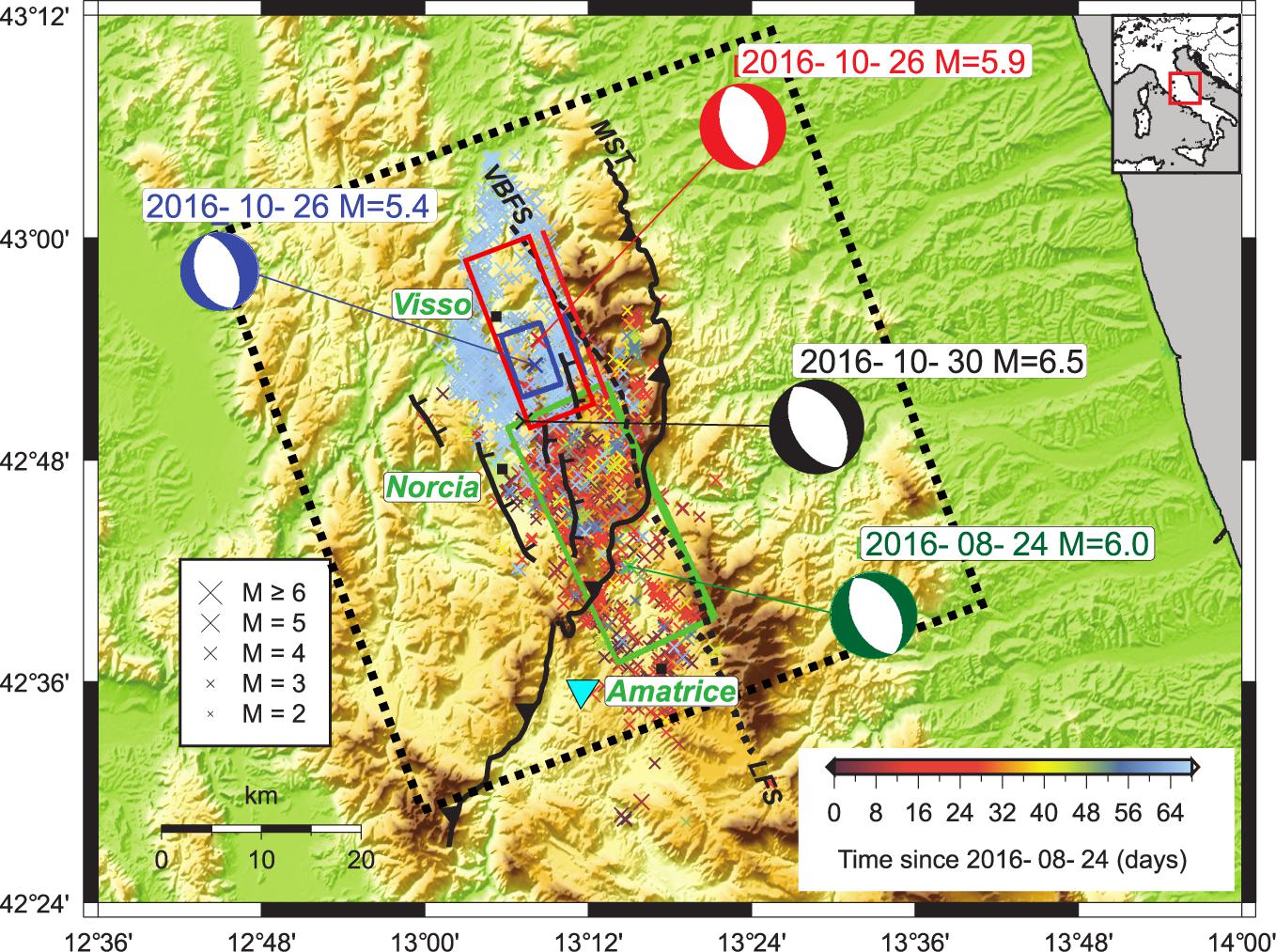
Figure 1. Geographic map, seismicity recorded from August 24, 2016 to October 26, 2016 (Chiaraluce et al., 2017). Thin dashed black lines show coseismic surface traces of the Vettore-Bove Fault System (VBFS) that ruptured during the AE (southern segment), the VE (northern and central segments) and NE (central and southern segments); dotted black lines show the Laga Fault System (LFS) that ruptured during the AE and NE; black line with triangles show the Mts. Sibillini Thrust (MST); black lines show main antithetic normal faults that bound the aftershock region (thicks denote the down-thrown block). The dashed black box identifies the upper face of the investigated volume. The beach balls indicate the fault mechanisms of the three analyzed events (see Table 1). Events (crosses) are color-coded according to their origin time. The inverted light-blue triangle identifies the Varoni 1 well.

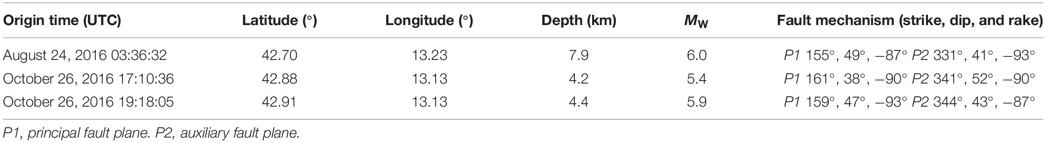
Table 1. Location, fault plane solutions, and moment magnitude for the three earthquakes in the Amatrice 2016 seismic sequence analyzed in the present study (Chiaraluce et al., 2017).

The main events of the sequence nucleated in the upper 8 km, within the Umbria-Marche carbonate multi-layer, and are characterized by normal fault mechanisms in accordance with the regional SW-NE trending extensional stress field (Chiaraluce et al., 2017). Source mechanisms of the three mainshocks, geodetic data, co-seismic surface ruptures, and aftershock distribution indicate the activation of NNW-SSE trending and WSW-dipping normal faults referable to two Quaternary systems: the Laga Fault system to the south and the Mt. Vettore-Mt. Bove system to the north [see Pizzi et al. (2017), among others] (Figure 1). The two segmented fault systems are crossed by the NNE-SSW trending oblique ramp of the Mts. Sibillini Thrust (MTS in Figure 1), which is a major regional arcuate structure of the Miocene-Pliocene compressional phase in central-northern Apennines (Pizzi et al., 2017). The aftershocks distribution (Improta et al., 2019) and the finite-fault inversion of geodetic data for the Norcia earthquake (Walters et al., 2018) indicate that main NE-dipping antithetic normal faults were also activated during the seismic sequence.

The present analysis aims at contributing to the understanding of the delayed triggering of the October 26, 2016, M_W = 5.4 and M_W = 5.9, Visso earthquakes. Previous studies have investigated some of the aforementioned triggering mechanisms for the AVN sequence. In particular, 3D Coulomb static stress redistribution has been computed by Convertito et al. (2017), Mildon et al. (2017), Tung and Masterlark (2018), Walters et al. (2018), Pino et al. (2019) and, although in all these cases the stress change value at the Visso hypocenters was enough to trigger them – if 0.01 MPa is assumed as threshold (e.g., Reasenberg and Simpson, 1992; King et al., 1994) – the delay remains unresolved. In addition, Tung and Masterlark (2018) have also shown that the afterslip (rate and state friction) and the viscoelastic mantle relaxation provide a negligible contribution to sequence evolution. Likewise, dynamic triggering, with associated in situ permeability increase and delayed peak in the local pore pressure rate, has proven to be an effective trigger (Convertito et al., 2017) but it seems to be inadequate to explain 60 days time delay.

Fluids flow and pore pressure diffusion has already been invoked as a viable mechanism to explain the evolution of two previous sequences in central Italy, i.e., the 1997 Umbria-Marche sequence (Antonioli et al., 2005) and 2009 L’Aquila sequence (Di Luccio et al., 2010; Malagnini et al., 2012), using a point source and isotropic or anisotropic hydraulic diffusivity assumption.

As for the AVN sequence, the fluid-earthquake interaction has been investigated by several authors using poro-elastic or diffusivity modeling. Tung and Masterlark (2018) interpreted spatial and temporal evolution of the aftershocks as the effect of pore fluid migration. These authors solved the fully coupled poroelastic equation in a 3D medium and using an extended source model searched for the optimal value of homogeneous and isotropic permeability that maximizes the value of the Coulomb stress change at the hypocentral location of the October 26, 2016 VEs, at their origin time. Their results indicate a permeability of 10^{–16 ± 0.7} m². Albano et al. (2019) used a simplified 2D poroelastic modeling along a W-E trending section orthogonal to the Amatrice causative fault to compute the coseismic and postseismic stress perturbations and predict the temporal evolution of the pore pressure change. Their main aim was to reproduce the temporal decay of the aftershocks observed after the AE. Permeability is assumed to increase with depth and is adjusted to optimize the fitting between the observed aftershock daily rate and the rate predicted with the simulated pore fluid diffusion. The obtained best fit permeability decreases from ∼5 × 10^–13 to ∼1 × 10^–13 m² between 0 and 20 km depth. To explain the poor spatial correlation found between the aftershocks’ distribution and the pattern of postseismic Coulomb stress change, the authors indicated the use of the 2-D modeling approximation (infinite fault length) and unmodeled features, such as heterogeneities and anisotropies in the elastic and hydraulic material properties. Walters et al. (2018) used a simple 1D diffusive model to verify whether the spatio-temporal evolution of the aftershocks occurred to the north of the Amatrice source was consistent with a diffusive process. Their forward modeling shows a diffusive-like temporal trend and the permeability fitting the aftershock triggering front is on the order of 10^–14m².

In summary, previous works face the problem by considering 3D crustal conductivity models, but homogeneous and isotropic (e.g., Tung and Masterlark, 2018) or 2D models with depth dependent conductivity (e.g., Albano et al., 2019).

Here we propose an additional modeling approach to study the role of fluids in triggering the Visso aftershocks. Our study roots on the following considerations and evidences:

(1) The geological and structural complexity of the Apennine chain and relative position of the causative fault and the aftershocks distribution require a 3D modeling of the crustal structure;

(2) In addition to variation with the depth, the conductivity is controlled by the widespread fracture systems in carbonate rocks in the Apennine chain, which underwent to multiphased contractional and extensional deformation. In particular, in the Apennines seismic belt, detailed studies on hydraulic properties of fractured carbonate reservoirs (Trice, 1999) indicate that open and conductive cracks and fractures, controlling effective fluid flow and propagation of the pore pressure perturbation over long distances, are those aligned by the active extensional stress field;

(3) The presence in this area of anisotropy in terms of conductivity, as revealed by S-wave splitting analysis (Pastori et al., 2019), previous studies of diffusivity related to aftershocks migration (e.g., Antonioli et al., 2005), and predicted by fault zone architecture (Caine et al., 1996).

We modeled pore pressure variations solving a one-way coupled pore pressure equation (Wang, 2000) in a 3D conductivity model. We performed a parametric study exploring isotropic and anisotropic models with conductivity values selected according to permeability profiles proposed by Kuang and Jiao (2014). For each investigated model we computed the pore pressure excess produced by the strain field associated with the AE at the hypocenter of the VEs occurred on 26 October, 2 h apart from each other and about 60 days since the AE.

Materials and Methods

Pore-pressure relaxation in an anisotropic and heterogeneous poro-elastic fluid-saturated medium is described by the Darcy’s equation that, under the hypothesis of one-way poroelastic coupling, is given by

where D_ij are the components of the hydraulic diffusivity tensor D, and x_j are the components of the coordinates vector of a given observation point with respect to the causative source. The one-way coupling approximation is justified when at least one of the following circumstances occurs: (i) under steady state conditions, (ii) the fluid compressibility is much greater than the frame compressibility, (iii) dealing with irrotational displacement fields in infinite or semi-infinite domain without body forces, (iv) in the presence of uniaxial strain and constant vertical stress (Wang, 2000). For the present study the one-way assumption is supported by the fact that the fluid considered is water whose compressibility is about 4.5 × 10^–10 Pa^–1 (assuming 2.2 GPa for compressibility modulus) while the frame compressibility is about 2.0 × 10^–11 Pa^–1 (using a compressibility modulus of about 50 GPa, see section Model parameterization). To evaluate the diffusion of pore fluid pressure P due to crustal deformation generated by the 24 August 2016, M_W = 6.0, earthquake, we used the numerical code PFlow (Wolf and Lee, 2009), which has been employed for applications similar to our study (Dyer et al., 2009; Wolf et al., 2010). PFlow performs 3D time-dependent numerical computation, based on linear finite elements for spatial discretization and implicit second order, finite difference in time. All the technical details about its implementation are reported in the Supplementary Material section. Since in elastic deformation stress is related to strain, crustal deformation is obtained from the Coulomb stress change field ΔCFS, which is given by:

where Δτ is the change in the shear stress, Δσ is the change in the normal stress and μ is the friction coefficient. In the present study, Coulomb stress changes were computed by using Coulomb 3.3 software (Lin and Stein, 2004). As reported by Harris (1998), μ ranges between 0.6 and 0.8 for most rocks. Following Albano et al. (2019) we assumed μ = 0.6, which is appropriate for fractured carbonate rocks (Scuderi and Collettini, 2016). Given the deformation, it is thus possible to obtain the initial pore pressure through the relation ΔP = −BΔε/G (Rice and Cleary, 1976), where Δε is the deformation, G is the bulk compressibility, and B is the Skempton coefficient (0 ≤ B ≤ 1). The initial pore pressure is then allowed to dissipate in model space over time.

The space-time evolution of pore pressure P can be computed by solving the Eq. (1) in the following form (Wang, 2000):

once initial and boundary conditions have been selected. The tensor k is the permeability tensor (k = DSη, being S the storage coefficient), η is the fluid viscosity, S_s is the specific storage coefficient, and Q is the fluid source term, as induced by seismic faulting.

Model Set-Up

In order to compute the space-time evolution of pore pressure, poroelastic and hydraulic properties of the medium must be defined. With reference to Eq. (3) these properties are: the bulk modulus, the Skempton coefficient B, the specific storage coefficient S_S, and the hydraulic conductivity tensor K = ρgk/η (being ρ the density of the fluid, k the permeability, and g the gravity acceleration). In addition, the initial condition must also be specified.

In this section we describe the procedure adopted to select the suitable parameters and to compute the initial conditions.

Strain Computation and Initial Condition

The modeling assumes that the initial event produces a stress/strain field in the volume surrounding the causative fault, whose shape depends on fault geometry and extent, and on slip distribution. To compute the ΔCFS field (Figure 2) and the strain field in the volume embedding the fault of the main event (24 August, Mw = 6.0) and those of the two 26 October Visso main aftershocks (Figure 1), we used the fault geometry and the slip distribution inferred from the InSAR and GPS data (Cheloni et al., 2017). We considered a volume of 60 km × 60 km × 28 km (dashed black box in Figure 1). We note the ΔCFS field in Figure 2A does not significantly change when a value of 0.7 or 0.8 is used as friction coefficient. Since the code PFlow operates in the principal axes system – that is, the conductivity tensor K is diagonal – for simplicity, we rotated the fault in such a way that one (Ky) of the two horizontal principal directions coincides with the strike direction of the source of the Amatrice earthquake (Table 1). The initial condition for the pore pressure at t = 0 is obtained by converting the strain in pore pressure by using the Skempton coefficient B, which is defined as the ratio between the induced pore pressure and the stress loading. The boundary conditions are of Neumann type (no flow) on the top of the volume and of Dirichlet type (constant pore pressure) on the other sides of the volume. Source parameters of the AE and of the two VEs are listed in Table 1. As for the Skempton coefficient, for high to moderate effective pressures (>10 MPa), values between 0.35 and 0.6 have been observed for saturated limestone and dolomite (Kumpel, 1991). A B-value of 0.5 was used by Astiz et al. (2014) for the geomechanical modeling of the Cavone carbonate reservoir in the northern Apennines, which consists of low to medium porosity, fractured Mesozoic carbonates similar to those drilled in the Amatrice area. Thus, for the modeling we adopted the same value for B. Nevertheless, due to the marked increase of B with decreasing effective pressure (carbonate rocks at low effective pressures <5 MPa show B-values up to 0.8; see Kumpel, 1991), larger values could be also considered for the uppermost sedimentary crust in the source region that according to local earthquake tomography surveys should consist of fractured, overpressurized carbonates (Chiarabba et al., 2018).

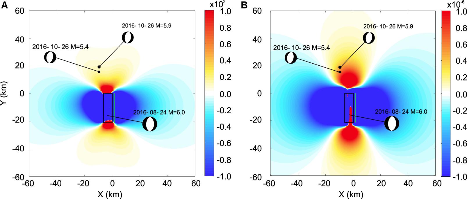
Figure 2. (A) Coulomb stress field (in kPa) following the August 24, 2016, M_W = 6.0, event, computed at 5 km depth. Receiver faults are assumed the same as the source (see Table 1). The black rectangle identifies the surface projection of the fault, while the green line represents the fault trace at surface. The epicenters of both the October 26, 2016, M_W = 5.4, and the October 26, 2016, M_W = 5.9, aftershocks are also displayed. The beach balls indicate the fault mechanisms of the three analyzed events (see Table 1). (B) Strain field – dilatation – computed at 5 km depth. Symbols are same as shown in (A).

Model Parameterization

The Amatrice and Visso earthquakes interested an area that spans two major structural domains, the Umbria-Marche thrust belt and the Laga foredeep domain, at the boundary between central and northern Apennines (Mazzoli et al., 2005). The upper crustal structure is very complex because thrusting involved different Meso-Cenozoic sedimentary sequences and the tectonic evolution was controlled by multiphased contractional and extensional deformation. Hydrocarbon exploration carried out in the 80s provided seismic reflection images of the thrust belt architecture, but due to the lack of oil discoveries the area was not investigated further and, consequently, specific information on the hydraulic properties of the drilled sedimentary rocks are lacking.

Seismic reflection profiles that cross the ruptured Vettore fault just in between the epicentres of the AE and VEs shocks show the Mts. Sibillini Thrust juxtaposing the Meso-Cenozoic carbonate multilayer of the Umbria-Marche succession on to Miocene foredeep basin deposits of the Laga domain (Porreca et al., 2018). In the hanging-wall of the Vettore fault, the thrust sheets stack is about 9 km thick and mainly formed by carbonate sequences consisting of slope-basinal limestones (Jurassic-Oligocene), platform limestones and dolomites (Triassic-Jurassic), evaporites (dolostones interbedded with anydrites, Triassic). The Triassic evaporites cover Permo-Triassic phyllitic basement (Bally et al., 1986) imaged locally at about 9 km depth (Porreca et al., 2018).

Field surveys and seismic reflection profiles evidence a complex interplay between Miocene-Pliocene reverse faults and mature Quaternary extensional systems, the latter formed by NNW-SSE striking synthetic and antithetic faults (Figure 1) that bound large intermontane basins. As a consequence, the Meso-Cenozoic carbonate multilayer is affected by pervasive systems of fractures and faults with a wide range of orientations, developed during the contractional tectonics and Quaternary extension (Pierantoni et al., 2013). The presence of thick, highly fractured zones is also suggested by seismic profiles, which show reflectivity and lateral coherence strongly decreasing in the carbonate crustal wedge comprised between the Vettore fault to the east and the antithetic normal faults to the west (Figure 1) (Porreca et al., 2018). Furthermore, the well Varoni 1 – located 5 km to the west of Amatrice town (Figure 1) – penetrated from 4.1 km to final depth (5.7 km) thick and strongly fractured zones in Triassic dolomites evidenced by total mud losses (well logs¹).

This geological complexity requires that the conductivity would be modeled by at least two layers. The first one 9 km thick for the carbonate sequences and corresponding to the seismogenic layer and a second one corresponding to the crystalline basement. Moreover, the presence of a widespread network of cracks and fractures in the carbonate rocks, developed during the contractional and extensional tectonic phases that interested this sector of the Apennines from Miocene to Quaternary, suggests an anisotropic behavior of the first layer. In particular, the cracks and fractures favorably oriented with respect to the active local stress field, mostly at high angle and NNW-SSE orientation, should be open and conductive, and allow the propagation of pore pressure perturbations over long distances.

This interpretation reconciles with the results of extensive S-wave splitting analysis carried out on numerous seismic stations installed in the epicentral area (Pastori et al., 2019). In particular, the mean fast S-wave direction is N146°, which is in agreement with the both NNW-SSE strike of the active normal faults (Figure 1) and the S_Hmax direction of the local stress field. Based on the spatio-temporal distribution of the anisotropic parameters and their relation to the stress field, Pastori et al. (2019) interpret the seismic anisotropy as due to a combination of two physical mechanisms: (i) stress-induced anisotropy (Crampin, 1991) caused by vertically aligned, opened and fluid-filled microcracks that pervade the carbonate rocks and are parallel to the direction of maximum horizontal stress S_Hmax, (ii) structural-induced anisotropy (Boness and Zoback, 2006) attributable to the alignment of parallel planar macroscopic fractures related mainly to major fault zones of the Quaternary extensional systems. Both sources of seismic anisotropy can be modeled by transverse isotropy, with S-waves polarized parallel and orthogonal to the planes normal to the formation symmetry axis (Boness and Zoback, 2006). However, the analysis does not allow to distinguish the predominant contribution between the stress- and structural-induced anisotropy because Quaternary faults tend to parallel the S_Hmax direction. The same dual physical mechanism was proposed by Pastori et al. (2009) for the Val d’Agri extensional basin in the southern Apennines, where the interpretation of S-wave splitting analysis benefits from detailed information on the physical/hydraulic properties and stress conditions of the local hydrocarbon carbonate reservoir.

Based on the observed dependence of the delay times on the hypocentral depth of the AVN aftershocks Pastori et al. (2019) concludes that the bulk of seismic anisotropy is confined in the upper crust (<10 km depth), within strongly fractured carbonate rocks, and above the brittle-ductile transition separating the Umbria-Marche carbonate multi-layer from the underlying metamorphic basement. Therefore, other possible sources of structural anisotropy such as parallel bedding planes, or preferential mineral alignment in the metamorphic mid-crust play a minimal role. The delay times presents very high average and normalized values (up to 0.75 s and 0.01 s/km, respectively) in a NNW-SSE trending strip delimited by the Mt. Vettore-Mt. Bove fault system and its antithetic faults that extend between the northern tip of the Laga Fault system and the source of the Visso largest event. This zone is interpreted as a heavily fractured and anisotropic crustal wedge, in which pressurized fluids are preferentially channeled.

To set an appropriate bulk modulus value for the study region, we used: (i) the sonic log of the deep exploration well Varoni 1 that drilled the entire Umbria-Marche carbonate multilayer, (ii) P-wave velocity profiles adopted for depth-conversion of time-migrated stack sections in the region (Bally et al., 1986, among others); (iii) the local earthquake tomography of Chiarabba et al. (2018) that gives insights into V_P and V_P/V_S (i.e., Poisson Ratio) in the source region, (iv) reference density values for the carbonate rocks and evaporites of the Umbria-Marche succession derived through laboratory measurements, density logs, and gravity data modeling (Girolami et al., 2014). Thus, by setting V_P = 5.0–6.4 km/s, density ρ = 2.5–2.7 × 10³ kg/m³, and Poisson Ratio between 0.29 (V_P/V_S = 1.85) and 0.32 (V_P/V_S = 1.95), we obtained bulk modulus values in the range 40–65 GPa. Lower values of the range attain to shallow slope-basinal carbonates, larger ones to Triassic evaporites.

Finally, as for the specific storage (S_S), values for moderately-to-highly fractured carbonates having low-to medium porosity range between 10^–6 and 10^–5 m^–1 (Younger, 1993). Using the compressibility values reported by Astiz et al. (2014) for the throughout studied oil/aqueous carbonate reservoir of the Cavone field in northern Apennines and assuming a porosity of 0.05, we obtained a value of 8 × 10^–5 m^–1 that falls within the reference interval of Younger (1993). For the poro-elastic modeling, we assumed a constant S_S value of 10^–6 m^–1 considering the overall low porosity of the Mesozoic carbonate rocks in the source region.

Direct estimates of rock hydraulic parameters lack in the study area. Thus, we investigated several permeability-depth models obtained according to the equation proposed by Kuang and Jiao (2014):

where z is the depth, k_s and k_r are the permeability at the surface and at greater depth, respectively, while the parameter α (dimensionless) specifies the decay rate and its value is −0.25 for the crust in general and −0.45 for disturbed crust. Using Eq. (4) to set up a permeability model requires that both k_s and k_r are specified for the area under study. To this aim, we explored k_s and k_r values on the basis of both information available for hydrocarbon reservoirs located in other regions of the Apennine seismic belt, sharing with the Amatrice-Visso area similar structural and lithological characteristics, and most general values present in literature. Concerning k_s, we refer to permeability values as large as 7 × 10^–14 m² obtained by Agosta et al. (2007) through laboratory measurements made on samples of a carbonate fault zone exposed at about 90 km distance from the epicentral area. On the other hand, for the area under study Albano et al. (2019) used k_s = 1 × 10^–12 m², thus in our parametric study we explored both these two values. In terms of conductivity, this corresponds to explore values in the range 10^–8 to 10^–6 m/s for the Mesozoic carbonate sequences. As for k_r, we explored values ranging between 1 × 10^–17 and 1 × 10^–15 m², which correspond to conductivity values of 10^–10–10^–8 m/s characterizing low permeable basement units (>9 km depth), consisting of phyllite and crystalline rocks (Townend and Zoback, 2000; Porreca et al., 2018).

To account for the expected anisotropy in the carbonate sequences we investigated values as large as 10^–5 to 10^–4 m/s, which are plausible for shallow, strongly fractured carbonate thrust sheets under low lithostatic pressure and for possible deeper fractured zones filled by fluids (Chiarabba et al., 2018), as those recognized in the source region of the Umbria-Marche 1997–1998 sequence (Miller et al., 2004).

Poroelastic Modeling

On the basis of what described in the previous section, in addition to a basic homogeneous conductivity model, we considered a two-layer model that accounts for the separation, at 9 km depth, between the Meso-Cenozoic carbonate multi-layer (i.e., the seismogenic layer) and the underlying basement units. For the layered model, we first considered the case in which each layer is homogeneous and isotropic and then we accounted for the anisotropic conductivity of the seismogenic layer. In particular, we considered larger conductivity values in the NNW-SSE direction, parallel to the conductive cracks kept open by the local extensional stress field – characterized by NNW-SSE trending S_Hmax (i.e., stress-induced anisotropy) – and to the major fault zones associated with the Quaternary extensional systems (i.e., structural-induced anisotropy).

For the isotropic and anisotropic layered models we explored the values of conductivity listed in Tables 2, 3, respectively, and used B = 0.5. The conductivity-depth profiles have been obtained by using in Eq. (4) k_s and k_r listed in the same Tables assuming α = −0.25. Then, the value assigned at each layer corresponds to the mean conductivity obtained by averaging the values of the profile in each layer.

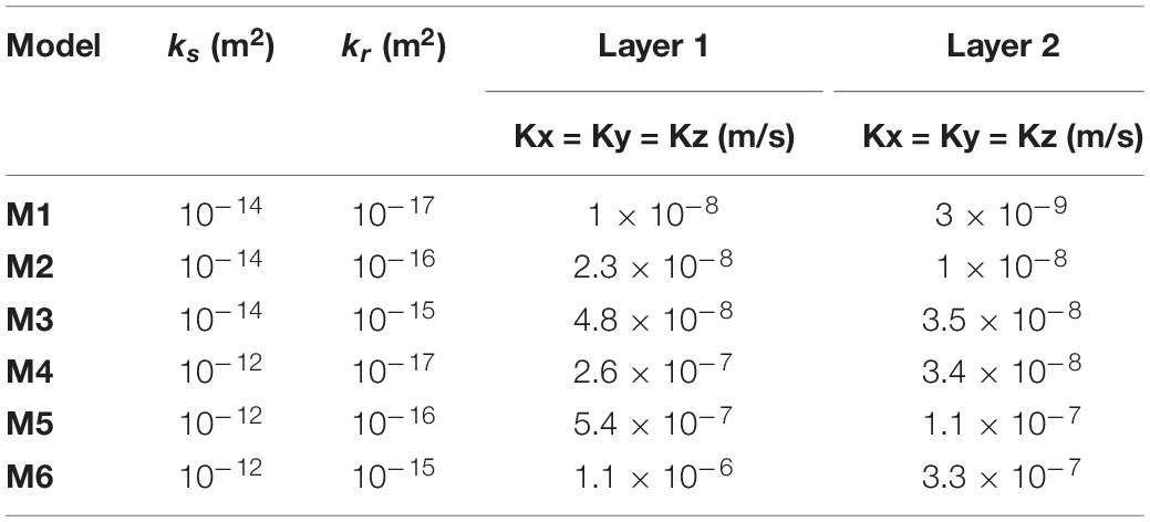
Table 2. Hydraulic parameters used to solve the 3D one-way coupled poroelastic diffusion equation: isotropic models.

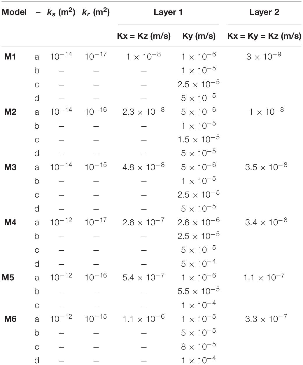
Table 3. Two-layer conductivity models used to solve the 3D one-way coupled poroelastic diffusion equation: anisotropic models.

For each model, using the PFlow code we computed the pore pressure as function of time at the hypocenter of the 26 October 2016, M_W = 5.4 and M_W = 5.9, Visso events.

As for the homogeneous and isotropic conductivity model, we first used the one proposed by Tung and Masterlark (2018) together with their hydraulic parameters. In particular, using their best permeability value 7.94(±0.13) × 10^–17 m², assuming a viscosity of 1 × 10^–3 (Pa × s) and a density of 1 g/cm³ the corresponding conductivity is K = 8 × 10^–10 m/s. As for the hydraulic parameters we used their values for Skempton coefficient B = 0.85, specific storage coefficient S_s = 4.4 × 10^–8 m^–1, and bulk compressibility G = 8.2 × 10^–12 Pa^–1.

The result of our simulation indicates that the pore pressure does not ever exceed the zero level and remains almost constant at about −8 kPa for the first aftershock and −10 kPa for the second one, in the whole considered period. By increasing the conductivity value by four orders of magnitude the pressure increases reaching its maximum value of 0.4 and 0.3 KPa at about 20 days for the two aftershocks, respectively. Constant pressure values are obtained also by considering all the isotropic models listed in Table 2 (Figures 3A,B).

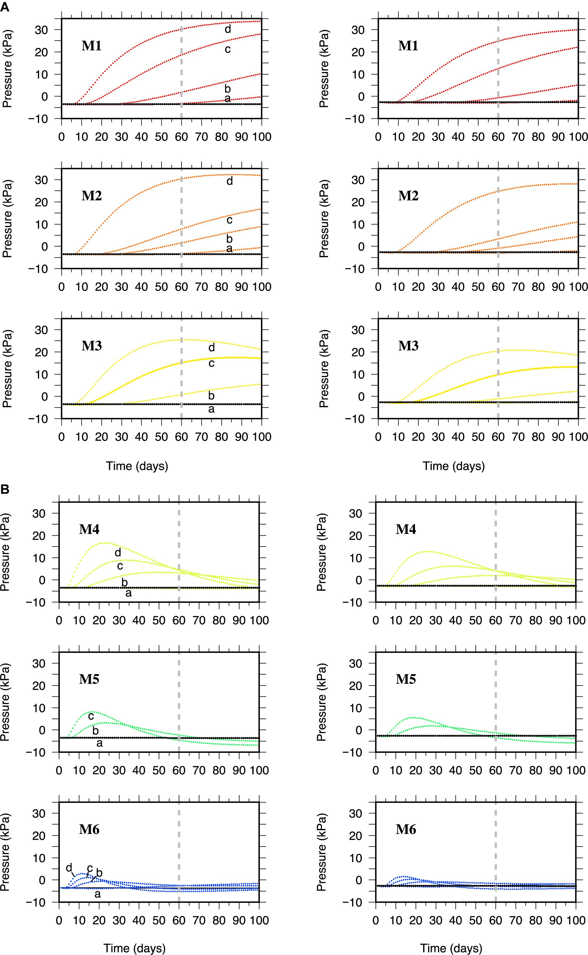
Figure 3. Pore pressure at Visso aftershocks hypocenter. (Left) panels refer to the 26 October 2016, M_W = 5.4, event and (Right) panels refer to the October 26, 2016, M_W = 5.9, event. Each panel refers to the model indicated. The curves have been obtained for the anisotropic conductivity models listed Table 3. The black horizontal lines correspond to the isotropic models listed in Table 2. The vertical dashed line in each panel identifies the occurrence time of the two Visso aftershocks.

The above results indicate that, assuming a one-way process, the eventual delayed triggering cannot be explained by pore pressure diffusion modeled in isotropic conductivity models, suggesting the intervention of anisotropic conductivity during the diffusion process. Given the assumed reference system this corresponds to a higher conductivity (Ky) along the NNW-trending W-dipping high-angle segments of the Mt. Vettore–Mt. Bove fault system and antithetic faults delimiting the aftershock zone (Figure 1). For all the isotropic models listed in Table 2, we performed a suite of simulations by increasing the conductivity Ky up to two order of magnitude with respect to Kx = Kz in the seismogenic layer. The investigated models are listed in Table 3.

For all the considered models, we verified that Ky values larger than 1 × 10^–4 m/s and lower than 5 × 10^–6 m/s provide at the hypocenter of the two Visso aftershocks, respectively, pore-pressure changes characterized by either a too early maximum or values below the triggering threshold, at the origin time of the two events (Figure 3). We found that, when Ky is on the order of 10^–5 m/s, models M1–M3 give rise to pore pressure changes with increase higher than 5–30 kPa (Figure 3A) at the time of the aftershocks. By adding any of these values to the estimated Coulomb static stress change (ΔCFS ∼ 10 kPa) (Figure 2A), the result exceeds the threshold assumed for the stress triggering. However, concerning the triggering threshold it should be considered that, although an optimal value does exist, there is no lower limit (Kilb et al., 2002). Note that the above models are characterized by K-values in the second layer ranging between 3 × 10^–9 and 3.5 × 10^–8 m/s. On the other hand, values of K on the order of 1 × 10^–7 m/s in the second layer, as for the case of models M5 and M6 (Figure 3B), cause fluids diffusing mainly downward. This effect dominates with respect to the anisotropy and by increasing Ky up to 1 × 10^–4 m/s, in order to overcame the vertical diffusion, the maximum of the computed pore pressure profile occurs too early compared to the aftershocks’ origin time. However, values on the order of 1 × 10^–7 m/s seem to be not consistent with those generally reported for the crystalline basement units (Townend and Zoback, 2000).

For the first 5–10 days, the pressure changes for both aftershocks, regardless of the conductivity model, are indistinguishable. Moreover, in the same time window they all show pore pressure decrease. This is due to the fact that the deformation generated in the considered volume by the AE, at the depths of the two aftershocks, produces dilatation causing the pore pressure to decrease. On the other hand, the spatial distribution of the strain produces pore pressure gradients between the two areas east and west of the AE source where there is a negative strain, therefore compression (ΔP > 0), and the area north of it, where there is a positive strain and therefore dilatation (ΔP < 0) (Figure 2B). These gradients are at the origin of the pore pressure diffusion toward the hypocenters of the aftershocks. In the following days, the pore pressure continues to grow and, based on the conductivity value, reaches either a value higher than the prescribed threshold for triggering an event or its maximum value at the origin time of the two aftershocks.

Finally, the parametric study suggests that pore pressure diffusion is effective when anisotropic conductivity models are considered. We note that, given the epistemic uncertainty on the conductivity for the area under study, it is hard to provide the optimal conductivity model able to explain the delayed triggering but a range of conductivity values can be identified. Moreover, the models listed in Table 3 and the associated pore pressure profiles shown in Figures 3A,B result from a combination of the considered permeability values for k_s and k_r in Eq. (4). Although representing a finite set out of all the possible models, the analysis allows to draw general conclusions about the main properties of the crustal structure in terms of conductivity. In particular, we find that all the models having conductivity in the first layer larger than 1 × 10^–8 m/s and up to 1 × 10^–7 m/s, and conductivity in the second layer on order of 10^–8 m/s, 10^–9 m/s, and also 10^–10 m/s (this latter not shown here), provide pore pressure profiles compatible with the delayed triggering if a first layer features anisotropy with Ky on the order of 10^–5 m/s.

We also verified that uncertainty on the hypocentral depth does not change the final conclusions. Indeed, as an example, for model M3, using as upper limit for the events depth those proposed by Chiaraluce et al. (2017) (4.2 and 4.4 km, respectively) varying the depth by ±1 km, results in pore pressure value higher than the triggering threshold (Figure 4). In addition, we note that using different values for the Skempton coefficient (0.5, 0.6, 0.7, and 0.8) does not change the time at which the maximum of the pore pressure arrives at the location of the two aftershocks, but increases the value of the pore pressure (Figure 4). This is because the Skempton coefficient controls how much of the initial strain is converted in pore pressure.

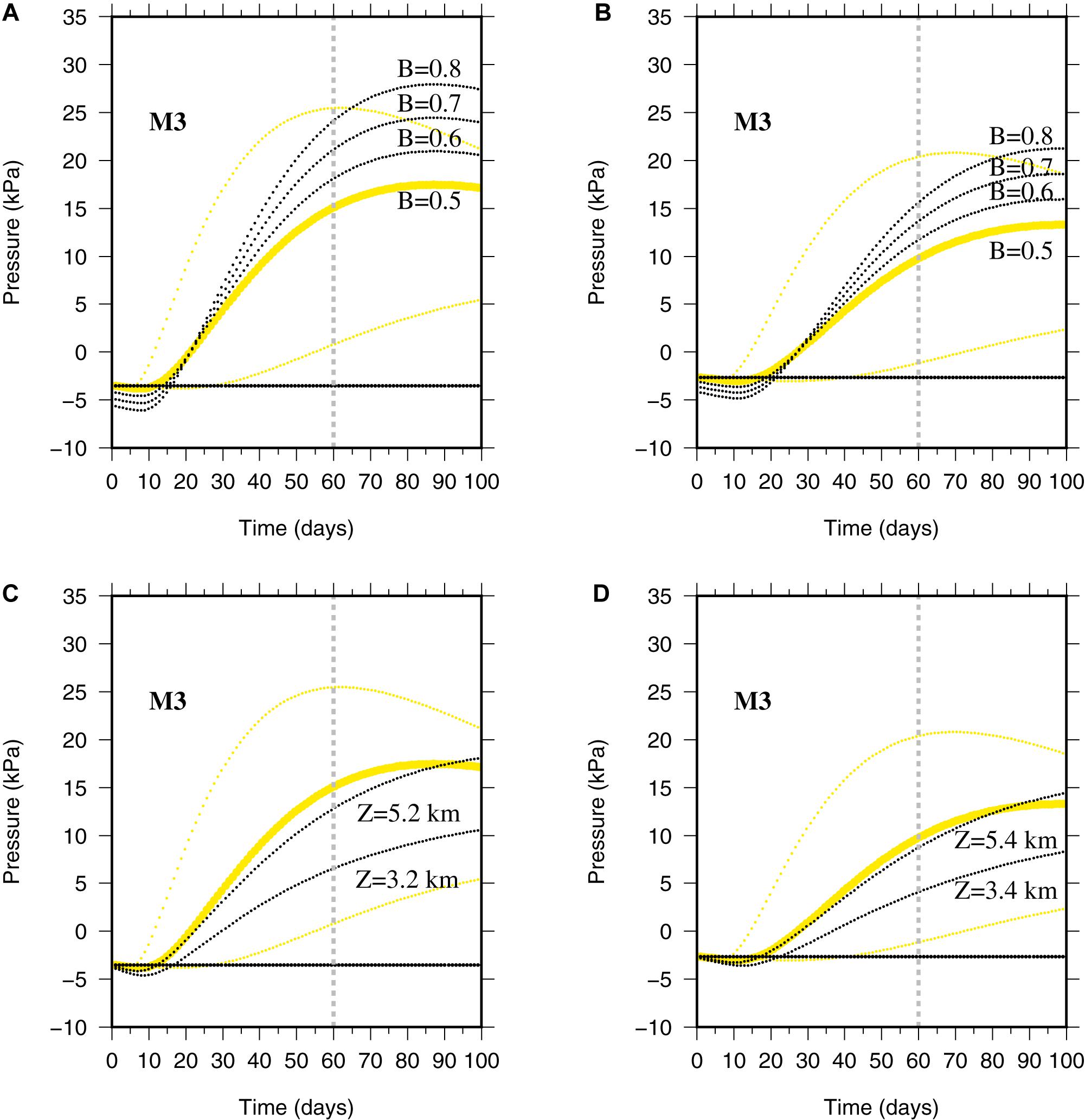
Figure 4. Testing different depths and Skempton coefficients. The upper panels (A,B) show pore pressure changes at the Visso aftershocks evaluated using the four Skempton B-values reported in the figure. Left panel refers to the October 26, 2016, M_W = 5.4, event and right panel refers to the October 26, 2016, M_W = 5.9, event. Lower panels (C,D) depict pore pressure as function of time computed at different hypocentral depths of the two Visso earthquakes. In all the panels the yellow line refers to the pore pressure profile computed using the models M3 listed in Table 3. The bold yellow lines refer to model M3c in Table 3 (ky = 2.5 × 10^–5 m/s). The black horizontal lines correspond to the isotropic model listed in Table 2.

Conclusion

We have investigated the delayed triggering of the two large aftershocks of the August 24, 2016, Amatrice, M_W = 6.0, earthquake occurred near Visso after 62 days and about 2 h apart. The Coulomb stress transfer analysis indicates that the two aftershocks are located in a positively stressed area (ΔCFF > 0) but it cannot account for the time delay. Among the possible delayed triggering mechanisms listed in the Introduction section, here we focused on the role of the fluids.

The mobilization of fluids during the Amatrice–Visso–Norcia sequence has been also reported by Barberio et al. (2017) who analyzed the hydrogeochemical changes in a set of springs in Central Apennines.

For the sequence investigated in the present study, the parametric analysis allowed to conclude that a set of possible conductivity models do exist that provide pore pressure values at the hypocenter of two Visso earthquakes occurred on 26 October, exceeding the generally assumed threshold of 0.01 MPa (e.g., Reasenberg and Simpson, 1992; King et al., 1994). In addition to the modeling proposed by Tung and Masterlark (2018) and Albano et al. (2019), we show that the time-space evolution of the seismic sequence can also be modeled by using a simpler one-way coupling diffusion process when an anisotropic conductivity model for the seismogenic layer is taken into account. In particular, we have verified that one-way poroelastic fluid diffusion is not effective to explain delayed earthquakes triggering when an isotropic conductivity model is used, but we show that this conclusion is overturned if anisotropic conductivity is introduced. However, for the study area, the anisotropic nature of the conductivity is consistent with: (i) the orientation of the major NNW-trending, W-dipping normal faults and associated antithetic faults activated during the seismic sequence, (ii) the direction of open and conductive fractures in the heavily fractured carbonate multilayer that are aligned by the local extensional stress field, as suggested by S-wave splitting analysis (Pastori et al., 2019). We remark that, aside from the specific conductivity values, the most effective models share as common feature the anisotropic nature of the conductivity. In particular, Ky should be about two or three orders of magnitude larger than Kx = Kz.

Incidentally, we note that although the hypocenter of the 30 October, M_W 6.5, Norcia earthquake is in between the August 24, 2016, Amatrice event and the two Visso aftershocks, it only occurred 4 days after these latter ones. This is an indication that the pore fluid pressure change following the Amatrice event was not enough to effectively reduce the normal stress and trigger the Norcia event, suggesting the contribute of additional favoring mechanisms. In this respect, Pino et al. (2019) have demonstrated that, in addition to the effect of the Amatrice earthquake, the two Visso events further increased the Coulomb stress in the central portion of the fault where the Norcia event nucleated, but those authors also invoked the intervention of a progressive weakening mechanism of the asperity contour through stress corrosion enhanced by fluids.

In conclusion, anisotropic conductivity is an actual characteristic of the crustal structure, in particular in tectonically active area. Although often neglected in model parameterization when fluid diffusion is analyzed, it should be taken into account.

Data Availability Statement

The datasets generated for this study are available on request to the corresponding author.

Author Contributions

VC, RDM, and NAP conceived the manuscript and performed the computations. LI made the geological and hydraulic parameterization. All authors wrote the manuscript.

Funding

This study was partially funded by the PRIN Project MATISSE (Bando, 2017, Prot. 20177EPPN2) and by Università del Sannio (Fondi di ricerca di Ateneo).

Conflict of Interest

The authors declare that the research was conducted in the absence of any commercial or financial relationships that could be construed as a potential conflict of interest.

Acknowledgments

We thank the reviewers for their valuable comments that allowed to improve the quality of the manuscript. The PFlow code is available by request to Prof. L. Wolf (wolflor@auburn.edu) or Prof. A. J. Meier (ajm@auburn.edu). The details of the analyzed events are available in the Supplementary Data of Chiaraluce et al. (2017). Figures were generated with Generic Mapping Tools (GMT; Wessel and Smith, 1991).

Supplementary Material

The Supplementary Material for this article can be found online at: https://www.frontiersin.org/articles/10.3389/feart.2020.541323/full#supplementary-material

Footnotes

1. ^ https://www.videpi.com/deposito/pozzi/profili/pdf/varoni_001.pdf

References

Agosta, F., Prasad, M., and Aydin, A. (2007). Physical properties of carbonate fault rocks, Fucino basin (Central Italy): implications for fault seal in platform carbonates. Geofluids 7, 19–32. doi: 10.1111/j.1468-8123.2006.00158.x
Albano, M., Barba, S., Saroli, M., Polcari, M., Bignami, C., Moro, M., et al. (2019). Aftershock rate and pore fluid diffusion: insights from the Amatrice-Visso-Norcia (Italy) 2016 seismic sequence. J. Geophys. Res. 124, 995–1015. doi: 10.1029/2018JB015677
Antonioli, A., Piccinini, D., Chiaraluce, L., and Cocco, M. (2005). Fluid flow and seismicity pattern: evidence from the 1997 Umbria-Marche (Central Italy) seismic sequence. Geophys. Res. Lett. 32:L10311.
Astiz, L., Dieterich, J. H., Frohlich, C., Hager, B. H., Juanes, R., and Shaw, J. H. (2014). On the Potential for Induced Seismicity at the Cavone Oilfield: Analysis of Geological and Geophysical Data, and Geomechanical Modeling. Report for the Laboratorio di Monitoraggio Cavone, 139 pp. Available online at: http://labcavone.it/documenti/32/allegatrapporto-studiogiacimento.pdf (accessed February 10, 2020).
Bally, A. W., Burbi, L., Cooper, C., and Ghelardoni, R. (1986). Balanced sections and seismic reflection profiles across the Central Apennines. Mem. Soc. Geol. Ital. 35, 257–310.
Barberio, M. D., Barbieri, M., Billi, A., Doglioni, C., and Petitta, M. (2017). Hydrogeochemical change before and during the 2016 Amatrice Norcia seismic sequence. Sci. Rep. 7:11735. doi: 10.1038/s41598-017-11990-8
Bizzarri, A. (2011). On the deterministic description of earthquakes. Rev. Geophys. 49:RG3002. doi: 10.1029/2011RG000356
Boness, N. L., and Zoback, M. D. (2006). A multiscale study of the mechanisms controlling shear velocity anisotropy in the San Andreas Fault observatory at Depth. Geophysics 71, 131–146. doi: 10.1016/j.epsl.2011.07.020
Brawn, M. R. M., and Ge, S. (2018). Distinguishing fluid flow path from pore pressure diffusion for induced seismicity. Bull. Seismic. Soc. Am. 108, 3684–3686. doi: 10.1785/0120180149
Caine, J. S., Evans, J. P., and Forster, C. B. (1996). Fault zone architecture and permeability structure. Geology 11, 1025–1028. doi: 10.1130/0091-7613
Cheloni, D., Albano, M., Antonioli, A., Anzidei, M., Atzori, S., Avallone, A., et al. (2017). Geodetic model of the 2016 Central Italy earthquake sequence inferred from InSAR and GPS data. Geophys. Res. Lett. 44, 6778–6787.
Chiarabba, C., De Gori, P., Cattaneo, M., Spallarossa, D., and Segou, M. (2018). Faults geometry and the role of fluids in the 2016–2017 Central Italy seismic sequence. Geophys. Res. Lett. 45, 6963–6971. doi: 10.1029/2018gl077485
Chiaraluce, L., Di Stefano, R., Tinti, E., Scognamiglio, L., Michele, M., Casarotti, E., et al. (2017). The 2016 Central Italy seismic sequence: a first look at the mainshocks, aftershocks and source models. Seismol. Res. Lett. 88, 757–771. doi: 10.1785/0220160221
Convertito, V., Catalli, F., and Emolo, A. (2013). Combining stress transfer and source directivity: the case of the 2012 Emilia seismic sequence. Sci. Rep. 3:3114. doi: 10.1038/srep03114
Convertito, V., De Matteis, R., and Emolo, A. (2016). Investigating triggering of the aftershocks of the 2014 Napa earthquake. Bull. Seism. Soc. Am. 106, 2063–2070. doi: 10.1785/0120160011
Convertito, V., De Matteis, R., and Pino, N. A. (2017). Evidence for static and dynamic triggering of seismicity following the 24 August 2016, MW = 6.0, Amatrice (Central Italy) earthquake. Pure App. Geophys. 174, 1–10.
Crampin, S. (1991). Wave propagation through fluid-filled inclusions of various shapes: interpretation of extensive-dilatancy anisotropy. Geophys. J. Int. 107, 611–623. doi: 10.1111/j.1365-246x.1991.tb05705.x
Di Luccio, F., Ventura, G., Di Giovambattista, R., Piscini, A., and Cinti, F. R. (2010). Normal faults and thrusts reactivated by deep fluids: the 6 April 2009 Mw 6.3 L’Aquila earthquake, central Italy. J. Geophys. Res. 115:B06315.
Doglioni, C., Barba, S., Carminati, E., and Riguzzi, F. (2014). Fault on-off versus coseismic fluids reaction. Geosci. Front. 5, 767–780. doi: 10.1016/j.gsf.2013.08.004
Dyer, G., Lee, M.-K., Wolf, L. W., and Meir, A. J. (2009). Numerical models of fluid-pressure changes resulting from the 1999 Chi-Chi earthquake, Taiwan, 09/15/2009-08/31/2010, GSA Abstracts with Programs Vol. 41, No. 7, Paper No. 170-14.
Gavrilenko, P. (2005). Hydromechanical coupling in response to earthquakes: on the possible consequences for aftershocks. Geophys. J. Int. 161, 113–129. doi: 10.1111/j.1365-246X.2005.02538.x
Girolami, C., Pauselli, C., and Barchi, M. R. (2014). “Gravitiy anomaly constraints for a crustal model of the northern Apennines,” in Proceedings of the Extended Abstracts of the GNGTS Meeting, Bologna.
Gomberg, J., Reasenberg, P. A., Bodin, P., and Harris, R. A. (2001). Earthquake triggering by seismic waves following the Landers and Hector Mine earthquakes. Nature 411, 462–466. doi: 10.1038/35078053
Harris, R. A. (1998). Introduction to special section: stress triggers, stress shadows, and implications for seismic hazard. J. Geophys. Res. 103, 24347–24358. doi: 10.1029/98JB01576
Helmstetter, A., and Shaw, B. E. (2009). Afterslip and aftershocks in the rate-and-state friction law. J. Geophys. Res. 114:B01308. doi: 10.1029/2007JB005077
Hsu, Y. J., Simons, M., Avouac, J. P., Galetzka, J., Sieh, K., Chlieh, M., et al. (2006). Frictional afterslip following the 2005 Nias-Simeulue earthquake, Sumatra. Science 312, 1921–1926. doi: 10.1126/science.1126960
Improta, L., Latorre, D., Margheriti, L., Nardi, A., Marchetti, A., Lombardi, A. M., et al. (2019). Multi-segment rupture of the 2016 Amatrice-Visso-Norcia seismic sequence (central Italy) constrained by the first high-quality catalog of Early Aftershocks. Sci. Rep. 9:6921. doi: 10.1038/s41598-019-43393-2
Kilb, D., Gomberg, J., and Bodin, P. (2000). Triggering of earthquake aftershocks by dynamic stresses. Nature 408, 570–574. doi: 10.1038/35046046
Kilb, D., Gomberg, J., and Bodin, P. (2002). Aftershock triggering by complete Coulomb stress changes. J. Geophys. Res. 107, ESE2-1–ESE2-14.
King, G. C., Stein, R. S., and Lin, J. (1994). Static stress changes and the triggering of earthquakes. Bull. Seismol. Soc. Am. 84, 935–953.
Kuang, X., and Jiao, J. J. (2014). An integrated permeability-depth model for Earth’s crust. Geophys. Res. Lett. 41, 7539–7545. doi: 10.1002/2014GL061999
Kumpel, H. J. (1991). Poroelasticity: parameters reviewed. Geophys. J. Int. 105, 783–799. doi: 10.1111/j.1365-246x.1991.tb00813.x
Lin, J., and Stein, R. S. (2004). Stress triggering in thrust and subduction earthquakes and stress interaction between the Southern San Andreas and nearby thrust and strike-slip faults. J. Geophys. Res. 109:B02323.
Malagnini, L., Lucente, F. P., De Gori, P., Akinci, A., and Munafo, I. (2012). Control of pore fluid pressure diffusion on fault failure mode: insights from the 2009 L’Aquila seismic sequence. J. Geophys. Res. 117:B05302. doi: 10.1029/2011JB008911
Mazzoli, S., Pierantoni, P. P., Borraccini, F., Paltrinieri, W., and Deiana, G. (2005). Geometry, segmentation pattern and displacement variations along a major Apennine thrust zone, central Italy. J. Struct. Geol. 27, 1940–1953. doi: 10.1016/j.jsg.2005.06.002
Mildon, Z. K., Roberts, G. P., Faure Walker, J. P., and Iezzi, F. (2017). Coulomb stress transfer and fault interaction over millennia on non-planar active normal faults: the MW 6.5-5.0 seismic sequence of 2016-2017, central Italy. Geophys. J. Int. 210, 1206–1218. doi: 10.1093/gji/ggx213
Miller, S. A., Collettini, C., Chiaraluce, L., Cocco, M., Barchi, M., and Kaus, B. J. P. (2004). Aftershocks driven by a high-pressure CO2 source at depth. Nature 427, 724–727. doi: 10.1038/nature02251
Miyazaki, S., Segall, P., Fukuda, J., and Kato, T. (2004). Space time distribution of afterslip following the 2003 Tokachi-oki earthquake: implications for variations in fault zone frictional properties. Geophys. Res.Lett. 31:L06623. doi: 10.1029/2003GL019410
Muir-Wood, R., and King, G. C. P. (1993). Hydrological signatures of earthquake strain. J. Geophys. Res. 98, 22035–22068. doi: 10.1029/93JB02219
Parsons, T. (2002). Global Omori law decay of triggered earthquakes: large aftershocks outside the classical aftershock zone. J. Geophys. Res. 107:B02199. doi: 10.1029/2001JB000646
Pastori, M., Baccheschi, P., and Margheriti, L. (2019). Shear wavesplitting evidence and relations withstress field and major faults from the “Amatrice-Visso-Norcia SeismicSequence”. Tectonics 38, 3351–3372. doi: 10.1029/2018TC005478
Pastori, M., Piccinini, D., Margheriti, L., Improta, L., Valoroso, L., Chiaraluce, L., et al. (2009). Stress aligned cracks in the upper crust of the Val d’Agri region as revealed by shear wave splitting. Geophys. J. Int. 179, 601–614. doi: 10.1111/j.1365-246X.2009.04302.x
Pierantoni, P. P., Deiana, G., and Galdenzi, S. (2013). Geological map of the sibillini mountains (Umbria-Marche Apennines, Italy). Ital. J. Geosci. 132, 497–520. doi: 10.3301/ijg.2013.08
Pino, N. A., Convertito, V., and Madariaga, R. (2019). Clock advance and magnitude limitation through fault interaction: the case of the 2016 central Italy earthquake sequence. Sci. Rep. 9:5005. doi: 10.1038/s41598-019-41453-1
Pizzi, A., Di Domenica, A., Gallovič, F., Luzi, L., and Puglia, R. (2017). Fault segmentation as constraint to the occurrence of the main shocks of the 2016 Central Italy seismic sequence. Tectonics 36, 2370–2387. doi: 10.1002/2017tc004652
Porreca, M., Minelli, G., Ercoli, M., Brobia, A., Mancinelli, P., Cruciani, F., et al. (2018). Seismic reflection profiles and subsurface geology of the area interested by the 2016–2017 earthquake sequence (Central Italy). Tectonics 37, 1116–1137. doi: 10.1002/2017TC00491
Reasenberg, P. A., and Simpson, R. W. (1992). Response of regional seismicity to the static stress change produced by the Loma Prieta earthquake. Science 255, 1687–1690. doi: 10.1126/science.255.5052.1687
Rice, J. R., and Cleary, M. P. (1976). Some basic stress diffusion solutions for fluid saturated elastic porous media with compressible constituents. Rev. Geophys. 14, 227–241. doi: 10.1029/rg014i002p00227
Scholz, C. H. (2002). The Mechanics of Earthquakes and Faulting, 2nd Edn, Cambridge: Cambridge University Press.
Scuderi, M. M., and Collettini, C. (2016). The role of fluid pressure in induced vs. triggered seismicity: insights from rock deformation experiments on carbonates. Sci. Rep. 6:24852. doi: 10.1038/srep24852
Shapiro, S. A., Patzig, R., Rothert, E., and Rindshwentner, J. (2003). Triggering of seismicity by pore-pressure perturbations: permeability-related signature of the phenomenon. Pure Appl. Geophys. 160, 1051–1066. doi: 10.1007/pl00012560
Stein, R. S. (1999). The role of stress transfer in earthquake occurrence. Nature 402, 605–609. doi: 10.1038/45144
Takai, K., Kumagai, H., and Fujii, N. (1999). Evidence for slow slip following a moderate-size earthquake (Mw = 5.7) in a subducting plate. Geophys. Res. Lett. 26, 2113–2116. doi: 10.1029/1999GL900465
Townend, J., and Zoback, M. D. (2000). How faulting keeps the crust strong. Geology 28, 399–402. doi: 10.1130/0091-7613(2000)028<0399:hfktcs>2.3.co;2
Tramelli, A., Convertito, V., Pino, N. A., Piochi, M., Troise, C., and De Natale, G. (2014). The 2012 Emilia (Italy) quasi-consecutive triggered mainshocks: implications for seismic hazard. Seismol. Res. Lett. 85:5. doi: 10.1785/0220140022
Trice, R. (1999). “Application of borehole image logs in constructing 3D static models of productive fracture network in the Apulian Platform, Southern Apennines,” in Borehole Imaging: Applications and Case Histories, Vol. 159, eds M. A. Lovell, G. Williamson, and P. K. Harvey (London: Geological Society), 156–176. doi: 10.1144/GSL.SP.1999.159.01.08
Tung, S., and Masterlark, T. (2018). Delayed poroelastic triggering of the 2016 October Visso earthquake by the August Amatrice earthquake, Italy. Geophys. Res. Lett. 45, 2221–2229. doi: 10.1002/2017GL076453
Walters, R. J., Gregory, L. C., Wedmore, L. N. J., Craig, T. J., Chen, J., Livio, F., et al. (2018). Dual control of fault intersections on stop-start rupture in the 2016 Central Italy seismic sequence. Earth Planet. Sci. Lett. 500, 1–14. doi: 10.1016/j.epsl.2018.07.043
Wang, H. F. (2000). Theory of Linear Poroelasticity with Applications to Geomechanics and Hydrogeology. Princeton, NJ: Princeton University Press.
Wessel, P., and Smith, W. H. F. (1991). Free software helps map and display data. Eos. Trans. AGU 72, 445–446.
Wolf, L. W., and Lee, M. (2009). 3-D Numerical Modeling of Coupled Crustal Deformationand Fluid Pressure Interactions. Final Technical Report, U. S. Geological Survey Award No. 08HQGR0031. Available online at: https://earthquake.usgs.gov/cfusion/external_grants/reports/08HQGR0031.pdf (accessed July 20, 2020).
Wolf, L. W., Lee, M., Meir, A., and Dyer, G. (2010). PFlow A 3-D numerical modeling tool for calculating fluid pressure diffusion from Coulomb strain. 09/15/2009-08/31/2010. Seismol. Res. Lett. 81:348.
Keywords: Coulomb stress transfer, anisotropic conductivity, pore-pressure diffusion, delayed triggering, Amatrice sequence
Citation: Convertito V, De Matteis R, Improta L and Pino NA (2020) Fluid-Triggered Aftershocks in an Anisotropic Hydraulic Conductivity Geological Complex: The Case of the 2016 Amatrice Sequence, Italy. Front. Earth Sci. 8:541323. doi: 10.3389/feart.2020.541323
Received: 08 March 2020; Accepted: 14 August 2020;
Published: 10 September 2020.
Edited by:
Max Rudolph, University of California, Davis, United StatesReviewed by:
Luca De Siena, Johannes Gutenberg University Mainz, GermanyCarlo Doglioni, Sapienza University of Rome, Italy
Copyright © 2020 Convertito, De Matteis, Improta and Pino. This is an open-access article distributed under the terms of the Creative Commons Attribution License (CC BY). The use, distribution or reproduction in other forums is permitted, provided the original author(s) and the copyright owner(s) are credited and that the original publication in this journal is cited, in accordance with accepted academic practice. No use, distribution or reproduction is permitted which does not comply with these terms.
*Correspondence: Vincenzo Convertito, vincenzo.convertito@ingv.it