Revealing Short-Term Precursors of the Strong M > 7 Earthquakes in Southern California From the Simulated Stress–Strain State Patterns Exploiting Geomechanical Model and Seismic Catalog Data

Introduction

The development of seismic hazard monitoring and prediction methods is crucial for preventing and mitigating the fatalities and damage caused by strong earthquakes. The primary focus of research in this field is linked to identification of precursors, preceding high-energy seismic events (Mogi, 1985; Sobolev and Ponomarev, 2003; Viti et al., 2003; Molchan and Keilis-Borok, 2008; Paresan et al., 2015; Bondur et al., 2018; Rundle et al., 2018 and references therein). Some precursors may be recognized from the anomalous behavior of various geophysical fields, including ones rendered by the dynamics of lineament systems (Bondur and Zverev, 2005; Paresan et al., 2015), variations of the ionosphere parameters (Liu et al., 2004; Bondur and Smirnov, 2005; Bondur et al., 2007; Singh et al., 2009), and other phenomena exhibiting increased activity before earthquakes. It is understood that the most effective approach for predicting significant seismic events is a joint comprehensive analysis of precursors of various physical nature recorded by ground-based and space instrumentation systems (Cenni et al., 2015 and references therein). However, an extreme complexity of the coupled processes and interaction mechanisms relating the subsurface mechanics during the stress accumulation (earthquake preparation) stage to potentially observable (geophysical) precursors makes the forecast a highly challenging goal, with relatively few examples of successful prediction.

The solid foundation of earthquake prediction would be the stress–strain state (SS) analysis, allowing for the identification of areas of elevated seismic risk employing regional-scale geomechanical models (Bondur et al., 2007; Bondur et al., 2010; Bondur et al., 2016). Making such models relevant requires reliable seismological data. Among the territories with elevated seismic risk, Southern California is one of the most studied in terms of tectonics, with high-quality seismic catalog data available.

The southern part of the US Pacific coast, in particular the state of California, as well as the adjacent territories of Mexico, is characterized by a significant level of seismic activity caused by the interaction of the Pacific and North American lithospheric plates, having the boundary along the San Andreas Fault (Wallace, 1990) (Figures 1 and 2). Given the high-density population of the area and the existing risk of strong and catastrophic seismic events, considerable attention has been paid for many decades to seismic monitoring and earthquake forecast in the region (Hutton et al., 2010). A seismological network deployed in Southern California (Clayton et al., 2015) provides a stream of high-resolution data, being processed, cataloged, and published by a number of specialized seismological centers and the US Geological Survey (USGS) nearly in real time (https://earthquake.usgs.gov/data/comcat/).

The main efforts of researchers aimed at short-term and medium-term earthquake forecast are related to statistical analysis of seismological datasets, resulting in probability estimates of seismic risk (Field et al., 2009; Field and Members of the 2014 WGCEP, 2015; Field et al., 2015; Ross et al., 2019). Although the models used in such an approach may incorporate data for the fault-block structure of the region, these do not provide a detailed image of elastic energy accumulation and redistribution in the subsurface. Another approach deals with local models of soil motion around the epicentral region, as derived from the earthquake focus mechanism post-quake data (Brandenberg et al., 2020).

At the same time, it is obvious that the physical basis for seismic risk assessment and forecast on a regional scale should exploit geomechanical models that take into account the structure, its heterogeneity, and current tectonic stresses (Turcotte, 1994). Some elements of this approach applied to Southern California have been discussed in Gomberg (1991), Williams and Richardson (1991), and Toda and Stein (2019). For identification of seismically hazardous zones, a joint analysis of the strength, stress state, and elastic energy distribution in the earth’s crust has been proposed (Garagash, 1991; Bondur et al., 2007).

To monitor the SS dynamics in relation to strong earthquakes in Southern California, back in 2009 we launched a numerical simulation study, employing both geomechanical modeling and actual seismological data (Bondur et al., 2010; Bondur et al., 2016; Bondur et al., 2017; Bondur et al., 2020). In our model, every new earthquake is treated as a new crustal defect, causing the stress–state redistribution and variation over time. By successive calculation of various SS attributes, the model makes it possible to trace the destruction and healing of the earth’s crust, reveal the patterns of elastic energy accumulation and relaxation, and ultimately identify the seismic precursors through imaging of elevated stress regions prior to strong (M > 7) shocks occurring in this territory.

In this article, we illustrate the application of this approach to particular seismic events of 2010 and 2019, being the strongest shocks in the region with M exceeding 7.

Materials and Methods

The results presented in this study have been obtained with a geomechanical modeling-based monitoring technique (Bondur et al., 2010; Bondur et al., 2016; Bondur et al., 2017; Bondur et al., 2020), allowing one to image and trace the SS evolution over the Southern California region during the period from 2009 to 2019, with the identification of SS precursor patterns preceding strong (M > 7) seismic events. At the core of this technique lies a three-dimensional (3D) geomechanical model simulating the crustal rock deformation within the latitudes between 31 and 36°N and longitudes between 114 and 121.2°W assuming the Mohr–Coulomb yield criterion.

The modeling domain with lateral dimensions of 645 km × 560 km is discretized by a 5-km × 5-km rectangular mesh. The earth’s crust and lithosphere are represented by a 6-layer structure within 0–35 km depth; the model includes the surface topography and crustal layers’ boundaries with realistic geometry specified according to available geological data. Each layer was assigned the specific values of Mohr–Coulomb model parameters, namely, the bulk modulus K, shear modulus G, cohesion c, and angle of internal friction φ (Table 1). The fault-block tectonics of a region was incorporated into the model using lineament analysis data by introducing a so-called crustal damage function $$g(x,y,z) that is applied to reduce the values of certain mechanical properties (elastic moduli, cohesion, and friction) in the corresponding mesh cells, for imitation of distracted portions of the crust associated with fault zones in any given layer, as

where $$_P0 is the constant initial value of the model property for the intact rock and $$κ is the small term (see Figure 2 and model properties maps in Figures 3 and 4). Damage function $$g(x,y)  represents the normalized spatial distribution of a dimensionless parameter (with values between 0 and 1), produced from fault maps, surface topography/bathymetry, and satellite imagery data (Bondur et al., 2010). At the earth’s surface, the degree of crustal destruction is assumed to be equal to 1 on the fault axis and 0 outside the zone of its influence, while in between it is approximated by the 2D spline function. Initially, the map of the damage function was constructed for the upper layer (L1) only, and then the damage distributions were calculated sequentially for deeper layers through the smoothing of the maps for upper ones, with the smoothing window size increasing with depth, forming a volumetric array $$g(x,y,z).

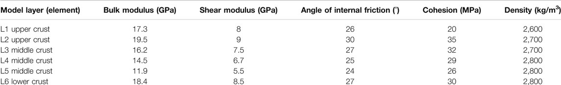
TABLE 1. Values of the material properties (Mohr–Coulomb model parameters) assumed for six laterally homogenous model layers at the initial stage of model construction, followed by application of “damage function” to produce heterogeneous property patterns (see Figures 3 and 4).

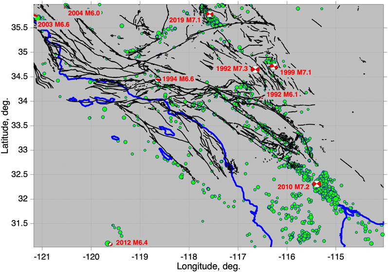
FIGURE 1. Fault tectonics (black lines, USGS database) and seismicity (green circles, ComCat database) in the study area. Beach balls and red text labels indicate earthquake mechanisms, year, and magnitude of major shocks during the time interval from 1990 to 2020.

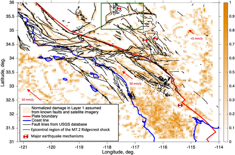
FIGURE 2. Fault tectonics and crustal destruction pattern (damage function) for the upper model layer. Red arrows show characteristic GPS-measured plate velocities in different parts of the study area.

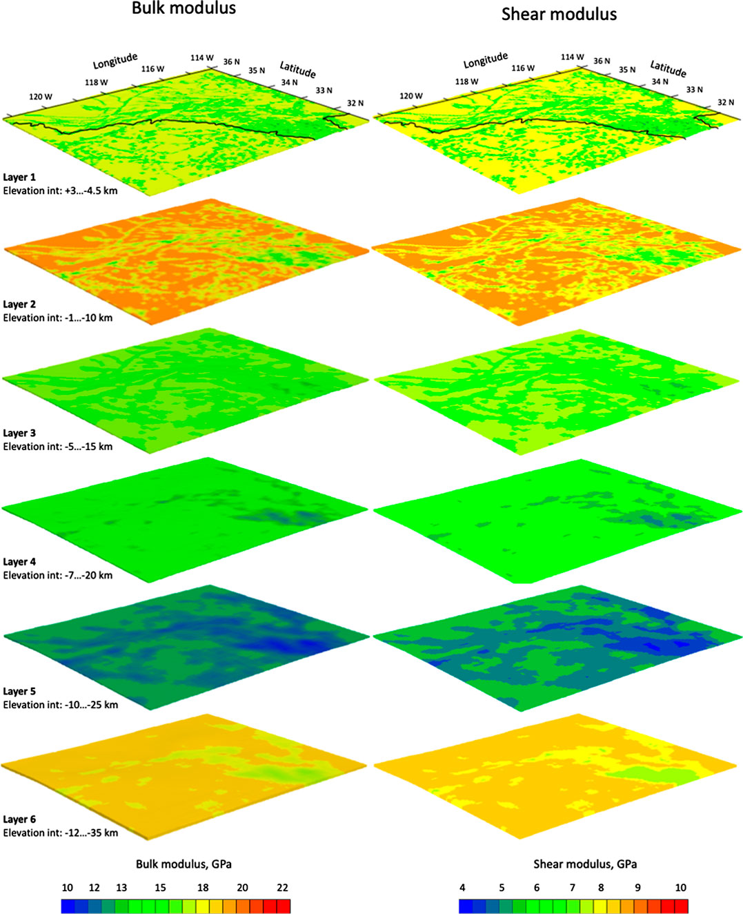
FIGURE 3. Initial model properties for six crustal layers: bulk (left column) and shear (right column) moduli distributions. Heterogeneous patterns reflect fault tectonics and reduced strength (assumed using the so-called damage function).

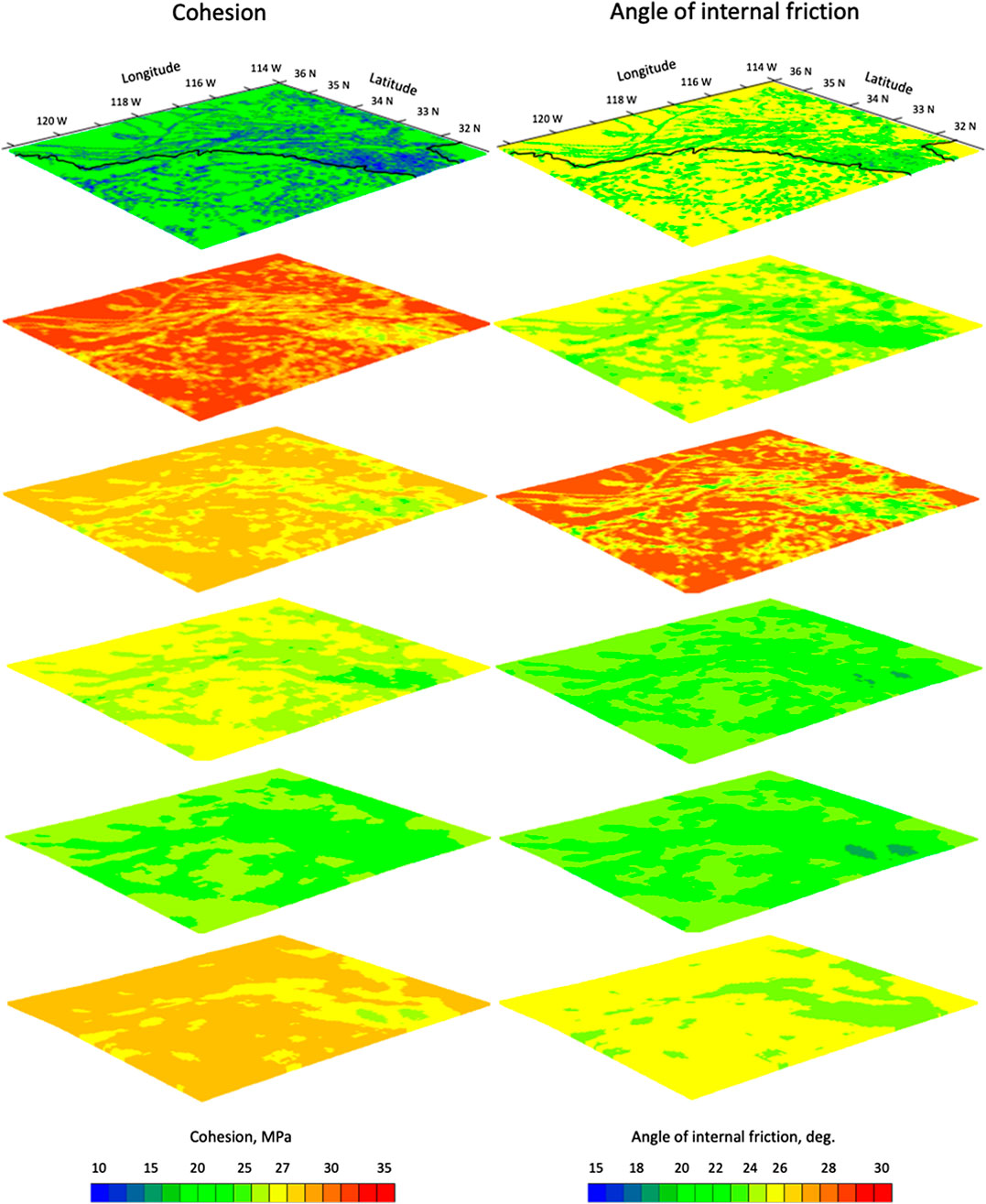
FIGURE 4. Initial model properties for six crustal layers: cohesion (left column) and angle of internal friction (right column) distributions. Heterogeneous patterns reflect fault tectonics and reduced strength (assumed using the so-called damage function).

At the initial stage, the “stationary” stress state of the model, $\text{SS}($x,y,z,_t0), is calculated under gravity load and the effect of regional tectonic forces assuming static approximation. Modeling is performed using FLAC3D software code (Itasca Consulting Group, 2006), solving the continuum mechanics equations with the explicit finite-difference method.

The stationary (or initial) state modeled as described above reflects the initial damage corresponding to fault-block tectonics; however, at this stage, the current seismic activity is ignored (see Figure 5).

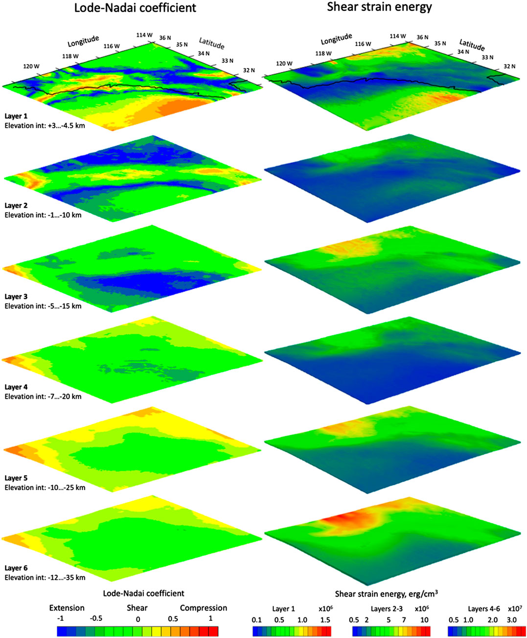
FIGURE 5. Initial stress state maps for six crustal layers calculated assuming gravity load and horizontal tectonic stresses according to the No-Net-Rotation NUVEL-1 model (Argus and Gordon, 1991): Lode–Nadai coefficient (left column) and shear strain energy (right column) maps.

The left column in Figure 5 presents the layered diagram of the Lode–Nadai coefficient, allowing one to classify the resulting stress distribution in terms of stress regime. This quantity is defined by the second and the third invariants of the stress tensors’ deviatoric part, and falls between −1 and +1. It equals −1 under pure tension and 1 under pure compression, while zero value is associated with pure shear.

The right-hand-side layered diagram in Figure 5 illustrates shear strain energy maps. Both quantities show elevated inhomogeneity in the upper layers compared to the lower ones and indicate complex overall patterns, defined by the interaction of Pacific and North American plates, complex geometry of crustal boundaries, and mosaic structure associated with fault tectonics in the study area.

The next (main) stage of calculation uses an iterative procedure to update the current state of the model:

This is achieved through subsequent update of the model geomechanical parameters, such as the bulk and shear moduli, cohesion, and friction angle, of those mesh elements which had been affected by seismic events during a 3-month time interval preceding the time point of the calculation. To achieve this, the foci locations taken from the seismic catalog are projected onto the model grid, and the released energy values E are estimated from the magnitude data M as

To evaluate the cumulative energy accommodated in each cell, the energies of all earthquakes falling within this cell are summed up over the 3-month period (about 4,000 individual shocks in average). Then, the smoothing is applied to the resulting energy distributions $$e(x,y,z,_ti), and the SS obtained at the previous iteration is used to calculate the updated damage function:

f_DM has the meaning of a transform converting energy array E at the current step into the updated damage function $$_gi+1=g(x,y,z,_ti+1). This is done with some algebra involving elements $$_σij of the stress tensor at the ith step. From those, the maximum shear stress is calculated:

and then, shear energy $$_ES and updated damage function g are evaluated based on the previous-step SS and current seismic energy distribution E:

In turn, g is applied to update the model parameters:

Specifically,

Here, P stands for any model property (bulk modulus K, shear modulus G, cohesion, or angle of friction φ); $\Delta$_Pi=_Pi−_Pi−1 indicates the damage-associated increment added to each property value at the previous step, while $$r=1/8 is the recovery factor applied to account for “rock healing” by $1/8$ of every 2 weeks (which means if no new earthquakes occur within a particular mesh element, its properties’ values return back to original values within 4 months), $$κ=0.3 is a small factor, and $$_gi+1=g(x,y,z,_ti+1) is the normalized damage function given by Eq. 7.

Finally, the new SS is computed from the corrected model:

Unlike the above transforms, $$_fSS is essentially a numerical solution to the equation of motion obtained with the FLAC^3D program code returning the full set of elements of the stress and strain tensors.

Thus, running the model implies serial evaluation of $$_fDM, $$_fMD, and $$_fSS transforms, yielding the updated datasets at each time step, that is, repeated half-monthly:

Once a new SS at the (i + 1)th step is calculated, the incremental part of the stresses is used to evaluate the strength parameter D, showing the proximity of the structure to its ultimate strength:

Here, $$_σ1,_σ3 stand for principal stresses and $$φ is the friction angle. The model regions with negative values of D at a given step are excluded from further analysis, since these indicate the stress relaxation with the crustal material state evolving in the opposite direction from strength limit (downgrading). At the same time, the patterns of positive values of D are visualized and analyzed in terms of absolute and relative (normalized by maximum value over a particular model layer or subdomain) distributions. Ultimately, all the above procedures are repeated for a new 3-month time-window, shifted by 1/2 month, forming a recursive loop (Figure 6).

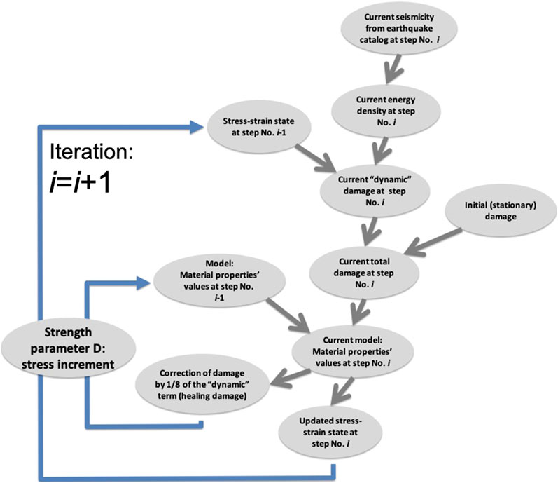
FIGURE 6. Stress–strain state simulation cycle and strength parameter monitoring.

Besides analysis of the strength parameter D, we also evaluate the time variation of maximum shear deformation in the upper and middle crust. Shear deformation is calculated as

where $$_εij are the strain tensor elements.

The main concept of such simulation-based monitoring consists in tracing the spatial migration of regions with abnormally high D and shear strain, and revealing of the correlation between migration patterns and seismic activity (here, we only include sufficiently strong shocks with M > 5.2). Besides, the time variations of maximum D values for individual layers and/or model subdomains are of particular interest.

Since 2009, such geomechanical simulation has been run continuously, with seismic magnitude data for all relevant earthquakes (M > 1) taken from the USGS ComCat catalog (https://earthquake.usgs.gov/data/comcat/). The monitoring results reported in this article include the SS patterns preceding the April 2010 M7.2 and July 2019 M7.1 earthquakes.

Results

To illustrate the approach described above, we focus on particular seismic events of 2010 and 2019, being the strongest shocks in the region with M exceeding 7.

Baja California 2010 Earthquake

Approximately 1 year after the start of our monitoring study, a strong M7.2. earthquake hit the Baja California region on April 4, 2010. This shock was preceded by elevation in strength parameter and specific pattern of its relocation during February–March 2010.

The spatial migration of the elevated-stress anomaly in terms of the strength parameter D within approximately 3 months before the event is given in Figure 7A. It can be seen that originally the anomaly emerges east of the future epicenter at a distance of R ∼ 20 km. Then, it migrates closer to the epicenter (R ∼ 10 km) and one extra anomaly arises northwest of the epicenter, where it follows the San Andreas fault (R ∼ 30 km). Next, the anomaly goes north to R ∼ 50 km, after which the high-stress region progressively moves toward the epicenter of the future M7.2 event.

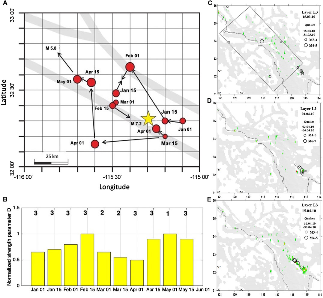
FIGURE 7. (A) Migration path of the strength parameter D maximum (red circles), as it is approaching the future epicenter of the M7.2 earthquake (yellow star) during January–July 2010. Gray-colored regions indicate zones of elevated rock damage; (B) variation in normalized maximum strength parameter D, calculated over the model domain; numbers above the bars indicate the corresponding model layer. (C)–(E) Particular states of middle crustal layer 3 in terms of D for March 15, April 1, and April 15, 2010, with black circles showing the epicenters of main shocks, occurring during this period.

Figure 7B shows the variation of the maximum normalized strength parameter D (evaluated across layers 1–3) during January−May 2010. A visible increase in D is observed during February, some 40–50 days prior to the main shock. Afterward, elevated D levels had been observed in late April–May, while the anomaly position left the earthquake area and no longer emerged close to it (within 50 km).

From the maps showing anomalies in D, it is possible to figure out that 20 days prior to the earthquake, no significant anomalies were observed over the entire model domain (Figure 7C), while such an anomaly emerged 15 days later (red point near the future epicenter, Figure 7D) and spread after the earthquake, forming the fault-associated region of distracted crust, where it remained during a few subsequent 2-week calculation cycles (Figure 7E).

Figure 8 demonstrates the behavior of shear strain for the same time samples, also showing the presence of anomalous displacements close to the epicenter a few days prior to the shock.

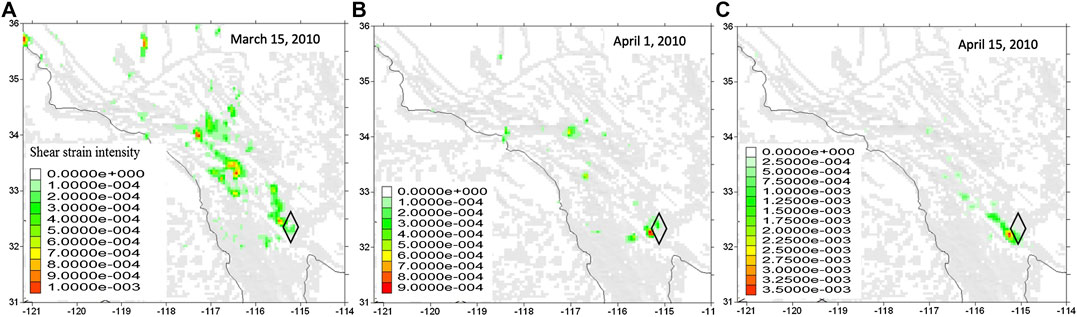
FIGURE 8. Shear strain mapped in middle crustal layer 2 corresponding to March 15, April 1, and April 15, 2010. The elevated strain is given as colored image map, with individual colorscales shown in each panel. Underlying grayscale corresponds to initial normalized damage. Black diamond shows the epicenter of the Baja California M7.2 shock.

We evaluated the stress regime for April 1, 2010, in terms of Lode–Nadai coefficient distribution in crustal layer 4 (Figure 9), in order to check whether it is consistent with the focal mechanism of the M7.2 Baja California earthquake, estimated from seismological data and known to be a strike-slip in the northwest–east-south direction (https://www.globalcmt.org/CMTsearch.html). Notably, we found that the epicenter falls within the whitish-colored cell with nearly zero value, which corresponds to shear setting.

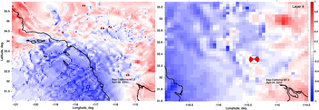
FIGURE 9. Lode–Nadai coefficient maps in layer 4 as of April 1, 2010, before the M7.2 Baja California earthquake for the entire study area (left panel) and epicentral region (right panel). Reddish color indicates compression, bluish—extension, and whitish—shear stress setting.

Ridgecrest July 2019 Earthquakes

In a similar way, we analyzed the computed stress–strain patterns for a few months prior to the 2019 Ridgecrest earthquakes, which had struck the region near the northern boundary of the study area. The main M7.1 shock occurred on July 5, 2019, and was preceded by an M6.4 foreshock on July 4, 2019 (Shelly, 2020). However, in this case, the spatial–temporal variation of the crustal strength parameter did not immediately reveal an isolated anomaly near the epicenter. Instead, a relatively faint anomaly was observed within the epicentral area (Figure 10) west of the epicenter starting from April 2019, accompanied by numerous higher-amplitude spots scattered all across the central part of the model domain. However, most of these spots displayed unstable behavior, changing their position chaotically or vanishing during model evolution. At the same time, the anomaly identified within the epicentral area remained steady with nearly no displacement during April, May, and June 2015, which attracted special attention to this region.

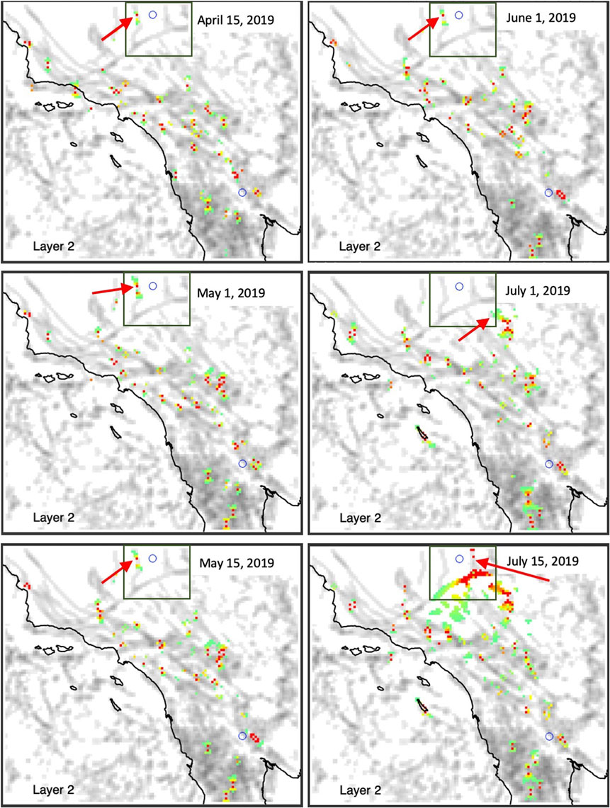
FIGURE 10. Strength parameter patterns for layer 2, plotted for a series of instants from April to June 2019. Grayscale corresponds to initial normalized damage, while colored spots indicate anomalous model cells with elevated D. Red arrows point at anomaly locations within the epicentral area (shown by dark-green rectangle), traced in the subsequent analysis (as demonstrated in Figure 11).

Figure 11A shows the path of migration sequence of the strength parameter anomaly for the period from January 1 to August 15, 2019. The epicenters of these two seismic events are shown by star symbols, while the gray-colored regions indicate the strength-reduced zones associated with tectonic faults. Tracing the anomaly migration, one can see that during January–March 2019, it was moving slowly in the southeastern corner of the epicentral subdomain and then jumped over to the northwest, approaching the epicenters of the July earthquakes. In May 2019 (i.e., 2 months before the seismic event), this anomaly reached its maximum value (Figure 11B), being located 30–35 km west of the epicenters.

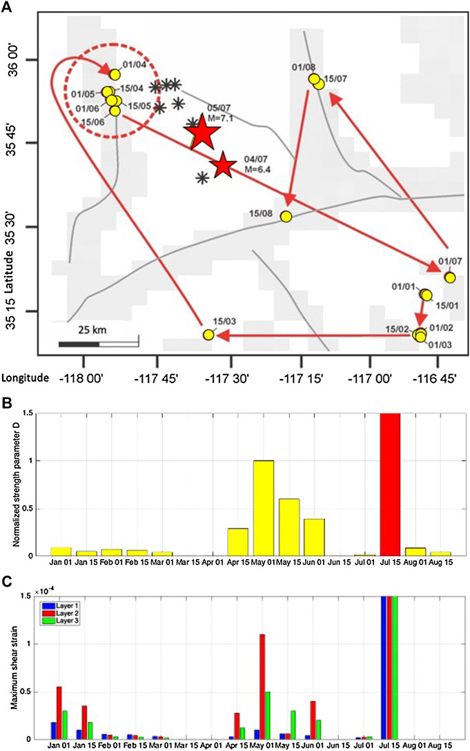
FIGURE 11. (A) Migration path of the strength parameter D maximum (yellow circles), as it is approaching the future epicenters of the M6.4 and M7.2 Ridgecrest earthquakes (red stars) during January–July 2019. Gray-colored regions indicate zones of elevated rock damage. Red dashed circle indicates the region where the maximum stays for a significantly long period over 2 months, which is identified as a precursor; (B) variation in the normalized maximum strength parameter D, calculated over the epicentral subdomain during January–August 2019; (C) plots of the maximum shear strain absolute values calculated for the three upper layers of the earth’s crust during January–July 2019, prior to the M7.1 Ridgecrest earthquake.

The time variation of the strength parameter D (Figure 11B) indicates the maximum elevated stress in the upper part of the earth’s crust at depths of about 7 km on May 1, 2019, that is, a half-month before the earthquake, when it significantly exceeded the background values. Besides, the zone of the maximum stress was located within the same area for as long as 2.5 months (from April to June 2019). We interpret this behavior as a precursor indicating that a strong seismic event had been in preparation in that area during that time. The steady identification of strength parameter maximum in nearly the same place over a substantially long time followed by a strong shock is definitely in sharp contrast with a normal (background) migration pattern, which is pretty chaotic, with relatively large moves all over the model domain. The occurrence of the M7.1 earthquake followed by an aftershock series caused the D parameter maximum to rocket in the mid-July. By August, it was back to background values.

In addition to revealing the anomaly in terms of D, it was found that starting early April till mid-June 2019, the maximum shear strain exhibited elevated values, with spatial location of the anomaly being in close proximity to the northwestern flank of the future earthquake fault line (staying in the region confined by the dotted line in Figure 11A). Figure 11C shows time variations of the maximum shear deformation calculated separately for each of the three upper layers of the earth’s crust during the period from February 1, 2019, to July 15, 2019. The maximum of the shear strain local anomaly is observed in May, 2 months before the M7.1 earthquake, which is similar to the behavior simulated strength parameter D. It is important to note that the deformation in layer 2, within a depth interval of nearly 3–7 km, exceeds the deformation in layer 3 (middle crust, 6–15 km depth). At the same time, in the upper part of the model (layer 1), deformation is of a lower level, which means the earthquake preparation process is not observable at the earth’s surface directly. It should be noticed that the quantities plotted in the above figure reflect only the relative SS dynamics and may not take into account some stationary parts of the deformation. However, in the subsequent analysis, it is possible to “calibrate” the model and adjust the obtained strain values based on available estimates of coseismic deformation in the earthquake source region.

Discussion

Having a decade-long series of SS distributions, with incremental parameters sampled half-monthly, we were to detect local anomalies months before the strong April 4, 2010, M7.2 earthquake and July 5, 2019, M7.1 earthquake. Both shocks are the only events with magnitude exceeding M = 7 that have occurred in the study area during the last decade. The revealed elevated-stress anomalies and the patterns of their migration prior to the shock can be considered as seismic precursors.

The described technique of SS monitoring in the Southern California region through geomechanical numerical simulation, launched in 2009, revealed some specific patterns of its behavior weeks and months prior to strong earthquakes. This provides substantial evidence for the efficiency of the approach based on the detailed geomechanical model updated continuously with current seismicity data. The earthquake foci parameters data, including even the weakest events (M > 1), characterize the process of crustal rupture and destruction and are critically important for the success of monitoring.

The core element of the modeling is the so-called damage parameter function, which determines the reduction in elastic constants of the crustal rocks due to destruction caused by earthquakes, which consists of the stationary part controlled by fault-block tectonics and the dynamic part associated with the ongoing seismic activity. Damage dynamics is estimated by summation of the impact of all earthquakes occurring over the 3-month interval, whose foci fall within a model. Each event is treated as a new crustal defect with dimensions determined by the Kasahara equation (Kasahara, 1981), and the entire simulation process allows for imaging and tracing the variations of elastic energy distribution. That reveals the patterns of its accumulation and dissipation, and enables identification of places where the rock state is of maximum proximity to ultimate strength, anomalies of strength parameter D.

Implementation of this quantity was proposed in our earlier research and seems to have a clear physical meaning, showing whether the stress state is getting closer to the strength limit (positive D) or farther from it (negative D). Although numerous other quantities describing the stress state might be employed to highlight areas of elevated stress, the stress elements alone are not indicative of possibility of failure. Analysis of D enables tracing the step-by-step variations of the model state, showing its evolution either toward failure or relaxation.

Since the SS includes both the stress (analyzed in terms of D) and strain parts (although related to each other via a constitutive model), we believe that some deformation-related quantity is useful for the analysis. As is known, strain accumulation may be considered as an earthquake precursor, and a significant amount of research has been focused on this subject. At the earth’s surface, deformations can be measured directly, with GPS-based or laser interferometry systems as well as compact strainmeters, mostly used in trenches and mines (Savage et al., 1981; Lyons and Sandwell, 2003; Fialko, 2006; Segall, 2010; Mazzotti et al., 2011). In Southern California, borehole deformation monitoring is performed in the Parkfield area (Johnston et al., 2006). However, such observations do not provide information on the spatial strain patterns deep in the subsurface, which is necessary for monitoring the stress–strain dynamics in connection with the prediction of strong earthquakes.

For the purpose of deformation analysis, we have chosen the shear strain due to its relation to shear, since most of the seismic shocks in the area are associated with this particular mechanism. An important feature seen from the shear strain distribution across layers indicates that no significant deformation anomaly emerges in the surface layer, even in the case of a fairly strong earthquake (M > 7), occurring in deeper layers of the crust. This explains the limited success of the forecast based on direct strain measurements.

However, to some extent, the strain anomalies can be revealed through geomechanical model-based simulations accounting for ongoing seismic shock magnitude data. As a result, the SS patterns are calculated, showing the way the rocks are being deformed across the entire modeling domain. Besides, this approach enables discrimination and further analysis of only those shear deformations that are not associated with regional-scale tectonic forces, but are rather caused by the current seismicity alone; the process of destruction; and post-quake healing of the earth’s crust.

Thus, by exemplifying two strong earthquakes in Southern California, namely, the M7.2 Baja California earthquake of April 4, 2010, and the Ridgecrest M7.1 main shock that occurred on July 5, 2019, we have shown that the proposed simulation-based method can be used for seismic hazard monitoring and prediction of strong shocks.

Data Availability Statement

Publicly available datasets were analyzed in this study. These data can be found here: https://earthquake.usgs.gov/data/comcat.

Author Contributions

VB initiated and guided the study and prepared the introductory part of the manuscript; MG proposed the concept of strength parameter tracing in application to Southern California and prepared the draft of the main body of the manuscript; IG implemented geomechanical modeling, providing the code to control SS calculation with FLAC software; and DA contributed with stress–strain data numerical analysis and visualization, along with final editing of the manuscript. All authors have read and approved the final manuscript.

Funding

The study was supported by the Institute for Scientific Research of Aerospace Monitoring “AEROCOSMOS” (Project No. АААА-А19-119081390037-2).

Conflict of Interest

The authors declare that the research was conducted in the absence of any commercial or financial relationships that could be construed as a potential conflict of interest.

References

Argus, D. F., and Gordon, R. G. (1991). No-net-rotation model of current plate velocities incorporating plate motion model NUVEL-1. Geophys. Res. Lett. 18, 2039–2042. doi: 10.1029/91gl01532
Bondur, V. G., Garagash, I. A., and Gokhberg, M. B. (2017). The dynamics of the stress state in Southern California based on the geomechanical model and current seismicity: short term earthquake prediction. Russ. J. Earth Sci. 17, ES105. doi: 10.2205/2017ES000596
Bondur, V. G., Gokhberg, M. B., Garagash, I. A., and Alekseev, D. A. (2020). A local anomaly of the stress state of the earth's crust before the strong earthquake (M = 7.1) of July 5, 2019, in the area of ridgecrest (Southern California). Dokl. Earth Sci. 490, 13–17. doi: 10.1134/S1028334X20010018
Bondur, V. G., Garagash, I. A., Gokhberg, M. B., Lapshin, V. M., Nechaev, Yu. V., Steblov, G. M., et al. (2007). Geomechanical models and ionospheric variations related to strongest earthquakes and weak influence of atmospheric pressure gradients. Dokl. Earth Sci. 414 (4), 666–669. doi: 10.1134/S1028334X07040381
Bondur, V. G., Garagash, I. A., Gokhber, M. B., Lapshin, V. M., and Nechaev, Y. V. (2010). Connection between variations of the stress–strain state of the Earth’s crust and seismic activity: the example of Southern California. Dokl. Earth Sci. 430 (1), 147–150. doi: 10.1134/S1028334X10010320
Bondur, V. G., Garagash, I. A., Gokhberg, M. B., and Rodkin, M. V. (2016). The evolution of the stress state in Southern California based on the geomechanical model and current seismicity. Izv. Phys. Solid Earth 52 (1), 117–128. doi: 10.1134/S1069351316010043
Bondur, V. G., and Smirnov, V. M. (2005). Method for monitoring seismically hazardous territories by ionospheric variations recorded by satellite navigation systems. Dokl. Earth Sci. 403 (5), 736–740.
Bondur, V. G., Tsidilina, M. N., Gaponova, E. V., and Voronova, O. S. (2018). Systematization of ionospheric, geodynamic, and thermal precursors of strong (M ≥ 6) earthquakes detected from space. Izv. Atmos. Ocean. Phys. 54 (9), 1172–1185. doi: 10.1134/S0001433818090475
Bondur, V. G., and Zverev, A. T. (2005) A method of earthquake forecast based on the lineament analysis of satellite images. Dokl. Earth Sci. 402 (4), 561–567.
Brandenberg, S. J., Stewart, J. P., Wang, P., Nweke, C. C., Hudson, K., Goulet, C. A., et al. (2020). Ground deformation data from GEER investigations of ridgecrest earthquake sequence. Seismol. Res. Lett. 91, 2024. doi: 10.1785/0220190291
Cenni, N., Viti, M., and Mantovani, E. (2015). Space geodetic data (GPS) and earthquake forecasting: examples from the Italian geodetic network. Boll. di Geofis. Teor. ed Appl. 56 (2), 129–150. doi: 10.4430/bgta0139
Clayton, R. W., Heaton, T., Kohler, M., Chandy, M., Guy, R., and Bunn, J. (2015). Community seismic network: a dense array to sense earthquake strong motion. Seismol. Res. Lett. 86, 1354–1363. doi: 10.1785/0220150094
Fialko, Y. (2006). Interseismic strain accumulation and the earthquake potential on the southern San Andreas fault system. Nature 441, 968–971. doi: 10.1038/nature04797
Field, E. H., Biasi, G. P., and Bird, P.; Working Group on California Earthquake Probabilities (2015). Long-term, time-dependent probabilities for the third uniform California earthquake rupture forecast (UCERF3). Bull. Seismol. Soc. Am. 105 (2A), 511–543. doi: 10.3133/fs20153009
Field, E. H., Dawson, T. E., Felzer, K. R., Gupta, V. A. D., Jordan, T. H., Parsons, T., et al. (2009). Uniform California earthquake rupture forecast, version 2 (UCERF 2). Bull. Seismol. Soc. Am. 99, 2053–2107. doi: 10.1785/0120080049
Field, E. H. and Members of the 2014 WGCEP. (2015). UCERF3: a new earthquake forecast for California’s complex fault system. U.S. Geological Survey, 2015–3009. doi: 10.3133/fs20153009
Garagash, I. A. (1991). Search of origination sites of strong earthquakes. Dokl. Akad. Nauk SSSR 318 (4), 862–867.
Gomberg, J. (1991). Seismicity and shear strain in the southern great basin of Nevada and California. J. Geophys. Res. 96 (B10), 16383–16399. doi: 10.1029/91jb01576
Hutton, K., Woessner, J., and Hauksson, E. (2010). Earthquake monitoring in southern California for seventy-seven years (1932–2008). Bull. Seismol. Soc. Am. 100 (2), 423–446. doi: 10.1785/0120090130
Itasca Consulting Group, Inc. (2006). FLAC3D—fast Lagrangian analysis of continua in 3 dimensions, version 3.1. User’s Manual. Minneapolis, MN: Itasca.
Johnston, M. J. S., Borcherdt, R. D., Linde, A. T., and Gladwin, M. T. (2006). Continuous borehole strain and pore pressure in the near field of the 28 September 2004 M 6.0 Parkfield, California, earthquake: implications for nucleation, fault response, earthquake prediction, and tremor. Bull. Seismol. Soc. Am. 96 (4B), S56–S72. doi: 10.1785/0120050822
Liu, J. Y., Chuo, Y. J., Shan, S. J., Tsai, Y. B., Chen, Y. I., Pulinets, S. A., et al. (2004). Pre-earthquake ionospheric anomalies registered by continuous GPS TEC measurements. Ann. Geophys. 22, 1585–1593. doi: 10.5194/angeo-22-1585-2004
Lyons, S., and Sandwell, D. (2003). Fault creep along the southern San Andreas from interferometric synthetic aperture radar, permanent scatterers, and stacking. J. Geophys. Res. 108, 2047. doi: 10.1029/2002jb001831
Mazzotti, S., Lucinda, L., Cassidy, J., Rogers, G., and Halchuk, S. (2011). Seismic hazard in western Canada from GPS strain rates versus earthquake catalog. J. Geophys. Res. 116, 12310. doi: 10.1029/2011JB008213
Molchan, G., and Keilis-Borok, V. (2008). Earthquake prediction: probabilistic aspect. Geophys. J. Int. 173, 1012–1017. doi: 10.1111/j.1365-246x.2008.03785.x
Peresan, A., Gorshkov, A., Soloviev, A., and Panza, G. F. (2015). The contribution of pattern recognition of seismic and morphostructural data to seismic hazard assessment. Boll. Geofis. Teor. Appl. 56 (2), 295–328. doi: 10.4430/bgta0141
Ross, Z. E., Trugman, D. T., Hauksson, E., and Shearer, P. M. (2019). Searching for hidden earthquakes in Southern California. Science 364, 767–771. doi: 10.1126/science.aaw6888
Rundle, J. B., Luginbuhl, M., Giguere, A., and Turcotte, D. L. (2018). Natural time, nowcasting and the physics of earthquakes: estimation of seismic risk to global megacities. Pure Appl. Geophys. 175, 647–660. doi: 10.1007/s00024-017-1720-x
Savage, J. C., Prescott, W. H., Lisowski, M., and King, N. E. (1981). Strain accumulation in southern California, 1973–1980. J. Geophys. Res. 86 (B8), 6991–7001. doi: 10.1029/JB086iB08p06991
Shelly, D. R. (2020). A high-resolution seismic catalog for the initial 2019 ridgecrest earthquake sequence: foreshocks, aftershocks, and faulting complexity. Seismol Res. Lett. 91, 1971. doi: 10.1785/0220190309
Singh, O. P., Chauhan, V., Singh, V., and Singh, B. (2009). Anomalous variation in total electron content (TEC) associated with earthquakes in India during September 2006–November 2007. Phys. Chem. Earth Parts A/B/C 34, 479–484. doi: 10.1016/j.pce.2008.07.012
Sobolev, G. A., and Ponomarev, A. V. (2003). Physics of the earthquakes and their precursors. Moscow, Russia: Nauka [in Russian].
Toda, S., Stein, R., and Stein, R. (2019). Ridgecrest earthquake shut down cross-fault aftershocks. Temblor. doi: 10.32858/temblor.043
Turcotte, D. L. (1994). “Crustal deformation and fractals, a review,” in Fractals and dynamic systems in geosciences. Editor J. H. Kruhl (Berlin, Germany: Springer-Verlag), 7–23.
Viti, M., D'Onza, F., Mantovani, E., Albarello, D., and Cenni, N. (2003). Post-seismic relaxation and earthquake triggering in the southern Adriatic region. Geophys. J. Int. 153, 645–657. doi: 10.1046/j.1365-246x.2003.01939.x
R. E. Wallace (Editor) (1990). The San Andreas fault system. California: U.S. Geological Survey. Professional Paper 1515. Available at: https://pubs.usgs.gov/pp/1990/1515/pp1515.pdf (Accessed August 31, 2020).
Keywords: geomechanical modeling, earth’s crust, stress–strain state, seismic risk, earthquakes, precursors, monitoring, South California
Citation: Bondur VG, Gokhberg MB, Garagash IA and Alekseev DA (2020) Revealing Short-Term Precursors of the Strong M > 7 Earthquakes in Southern California From the Simulated Stress–Strain State Patterns Exploiting Geomechanical Model and Seismic Catalog Data. Front. Earth Sci. 8:571700. doi: 10.3389/feart.2020.571700
Received: 11 June 2020; Accepted: 18 August 2020;
Published: 09 September 2020.
Edited by:
Giovanni Martinelli, National Institute of Geophysics and Volcanology, ItalyReviewed by:
Marcello Viti, University of Siena, ItalyMing-Ching T. Kuo, National Cheng Kung University, Taiwan
Copyright © 2020 Bondur, Gokhberg, Garagash and Alekseev. This is an open-access article distributed under the terms of the Creative Commons Attribution License (CC BY). The use, distribution or reproduction in other forums is permitted, provided the original author(s) and the copyright owner(s) are credited and that the original publication in this journal is cited, in accordance with accepted academic practice. No use, distribution or reproduction is permitted which does not comply with these terms.
*Correspondence: Dmitry A. Alekseev, alexeevgeo@gmail.com