the Creative Commons Attribution 4.0 License.
the Creative Commons Attribution 4.0 License.
 | 04 Sep 2020
Vegetation influence and environmental controls on greenhouse gas fluxes from a drained thermokarst lake in the western Canadian Arctic
June Skeeter
Andreas Christen
Andrée-Anne Laforce
Elyn Humphreys
Greg Henry
Thermokarst features are widespread in ice-rich regions of the circumpolar Arctic. The rate of thermokarst lake formation and drainage is anticipated to accelerate as the climate warms. However, it is uncertain how these dynamic features impact the terrestrial Arctic carbon cycle. Methane (CH4) and carbon dioxide (CO2) fluxes were measured during peak growing season using eddy covariance and chambers at Illisarvik, a 0.16 km2 thermokarst lake basin that was experimentally drained in 1978 on Richards Island, Northwest Territories, Canada. Vegetation in the basin differs markedly from the surrounding dwarf-shrub tundra and included patches of tall shrubs, grasses, and sedges with some bare ground and a small pond in the centre. During the peak growing season, temperature and wind conditions were highly variable, and soil water content decreased steadily. Basin-scaled net ecosystem CO2 exchange (NEE) measured by eddy covariance was −1.5 [CI95 %±0.2] g C−CO2 ; NEE followed a marked diurnal pattern with no day-to-day trend during the study period. Variations in half-hourly NEE were primarily controlled by photosynthetic photon flux density and influenced by vapour pressure deficit, volumetric water content, and the presence of shrubs within the flux tower footprint, which varied with wind direction. Net methane exchange (NME) was low (8.7 [CI95 %±0.4] ) and had little impact on the growing season carbon balance of the basin. NME displayed high spatial variability, and sedge areas in the basin were the strongest source of CH4 while upland areas outside the basin were a net sink. Soil moisture and temperature were the main environmental factors influencing NME. Presently, Illisarvik is a carbon sink during the peak growing season. However, these results suggest that rates of growing season CO2 and CH4 exchange rates may change as the basin's vegetation community continues to evolve.


The northern permafrost region stores approximately 50 % of global organic soil carbon in 16 % of the terrestrial land area (Tarnocai et al., 2009). Thermokarst landscapes account for approximately 20 % of the land area in this region and hold about half of its organic soil carbon (Olefeldt et al., 2013). Lake thermokarst landscapes are widespread in poorly drained, sedimentary permafrost lowlands with excess ground ice volume and constitute about a third of all thermokarst area (French, 2017; Olefeldt et al., 2013). Thermokarst lakes are a prominent landscape feature of the western Canadian Arctic (Mackay, 1999; Marsh et al. 2009; Lantz and Turner, 2015). These lakes drain, sometimes catastrophically, forming drained thermokarst lake basins (DTLBs) via bank overflow, ice wedge erosion, coastal erosion, and stream migration (Billings and Peterson, 1980; Mackay, 1999). Lake formation and drainage are a natural part of the thaw lake cycle, but it is anticipated that climate change will accelerate or disturb this cycle, potentially altering the regional carbon balance (Jones et al., 2018).
Net ecosystem exchange (NEE), ecosystem respiration (ER), and gross primary productivity (GPP), where , are lower in the Arctic than warmer regions but have significant seasonal cycles and variability between vegetation types (Virkkala et al., 2018). Future trajectories in NEE will in large part be governed by ER (Biasi et al., 2008; Cahoon et al., 2012). Dominant vegetation types in the western Canadian Arctic are erect-shrub tundra and wetlands (Walker et al., 2005). Growing season NEE is typically negative across these units throughout the Arctic, indicating a net CO2 sink as GPP exceeds ER in part due to cold and/or anoxic soil conditions (Virkkala et al., 2018; Lafleur et al., 2012). Annual NEE can be positive or negative with large variation in GPP linked to annual weather variability (Virkkala et al., 2018, McGuire et al., 2009). Arctic net methane exchange (NME) is positive because wetland areas are strong methane (CH4) sources while upland areas with better drainage can be net sinks (Whalen and Reeburgh, 1990; McGuire et al., 2009; Sturtevant and Oechel, 2013).
Thermokarst lakes are well-recognized sources of CH4 (Walter et al., 2007), which is 28 times as potent as carbon dioxide (CO2) on a 100-year timescale (IPCC, 2014). Thermokarst lake formation and expansion is expected to exert a positive feedback on climate change and accelerate Arctic warming in the near term, but modelling suggests that drainage may limit expansion and result in decreased lake area by the end of the century (van Huissteden et al., 2011). Post drainage, DTLBs undergo rapid ecological succession. In colder tundra environments, wet meadows or polygonal landscapes dominated by sedges, grasses, and rushes will form (Lara et al., 2015). In slightly warmer boreal and transitional regions, DTLBs often become dominated by willows and other shrubs (Lantz and Turner, 2015).
Carbon exchange in DTLBs of various ages has been examined in a few studies, almost exclusively focused on the Barrow Peninsula in northern Alaska. DTLB NEE during the growing season is negative with the greatest CO2 uptake in younger basins and decreasing net uptake as basins age in this region (Zona et al., 2010; Zulueta et al., 2011; Sturtevant and Oechel, 2013; Lara et al., 2015). DTLB source–sink strength of CH4 was found to be highly variable depending on vegetation and ground conditions (Lara et al., 2015). NME is highest in wet meadows and remnant ponds but considerably reduced in areas with better drainage (Zona et al., 2009, 2012; Lara et al., 2015). There may be regional variations in the carbon balance of DTLBs. For example, a shrub-dominated ancient DTLB known as Katyk in the Indigirka lowlands of Siberia shows considerably higher growing season carbon uptake than young Alaskan DTLBs with comparable NME (van der Molen et al., 2007; Parmentier et al., 2011). Similarly, DTLBs in the western Canadian Arctic may have different carbon fluxes than Alaskan DTLBs due to differences in climate and vegetation composition.
In this study, fluxes of CO2 and CH4 were measured at Illisarvik, an experimentally drained thermokarst lake basin on Richards Island in the western Canadian Arctic, Northwest Territories, Canada. Fluxes of CO2 and CH4 were measured during the peak growing season using a combination of closed chamber and eddy covariance (EC) measurements. NEE was calculated from fluxes, and storage change and was separated into ER and GPP. Here we report on (1) the spatial and temporal variability of the NEE and NME during the growing season, (2) the vegetation and environmental factors influencing NEE and NME, (3) how the growing season carbon balance at Illisarvik compares to other DTLBs, and (4) potential future carbon balance trajectories as Illisarvik's vegetation communities continue to evolve.
2.1 Study site and data collection
The study took place at Illisarvik, a DTLB on Richards Island (69∘28′47.5′′ N, 134∘35′18.7′′ W), which was drained experimentally in 1978 (Mackay, 1997). Illisarvik has since served as the focus of studies on permafrost growth, active layer development, and vegetation succession (Ovenden, 1986; Mackay and Burn, 2002; O'Neil and Burn, 2012; Wilson et al., 2019). At the nearby Tuktoyaktuk climate station mean annual air temperature (Ta) is −10.1 ∘C, July is the warmest month with a mean of 11 ∘C, and January is the coldest at −27 ∘C. Mean annual precipitation is 160.7 mm yr−1, the majority falling as rain in the summer and autumn. Snow cover typically lasts from mid-September or early October to late May (Environment Canada, 2016). Tuktoyaktuk is 60 km east of Illisarvik and in similar proximity to the coast so the climatology is expected to be similar at Illisarvik.
Table 1Dominant species or landscape feature within the vegetation/cover classes. Unit codes correspond to the map in Fig. 1a.
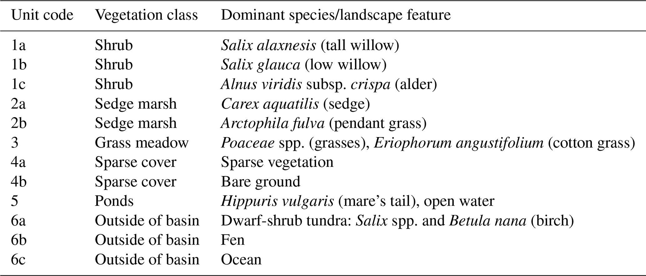
In the 39 years since drainage, Illisarvik has undergone rapid vegetation succession. After drainage, there were two remnant ponds. In the first 5 years after drainage, vegetation colonized the basin margins and wetter areas (Ovenden, 1986). By 1999, low vegetation had proliferated across most of the basin and taller willows had become established along the basin margins (Mackay and Burn; 2002). By 2010, some of the willows had grown to be 3 m in height (O'Neil and Burn; 2012). Current vegetation at Illisarvik is diverse relative to the dwarf-shrub tundra of the surrounding uplands (Table 1); the basin hosts a mix of woody shrubs (Salix spp., Betula spp., and Alnus spp.), wetland vegetation (Carex aquatilis, Arctophila fulva, etc.), and various grasses (Pocacea spp.) (Wilson et al., 2019). The basin is partly ringed by a terrace of peat that formed after a partial drainage event ∼5000 years BP and supports vegetation similar to the uplands (Michel et al., 1989). An ancient DTLB is located 100 m to the south of the Illisarvik basin, and the Arctic Ocean is to the west of the basin, separated by a ridge of upland tundra about 50 m wide at its narrowest (Fig. 1).
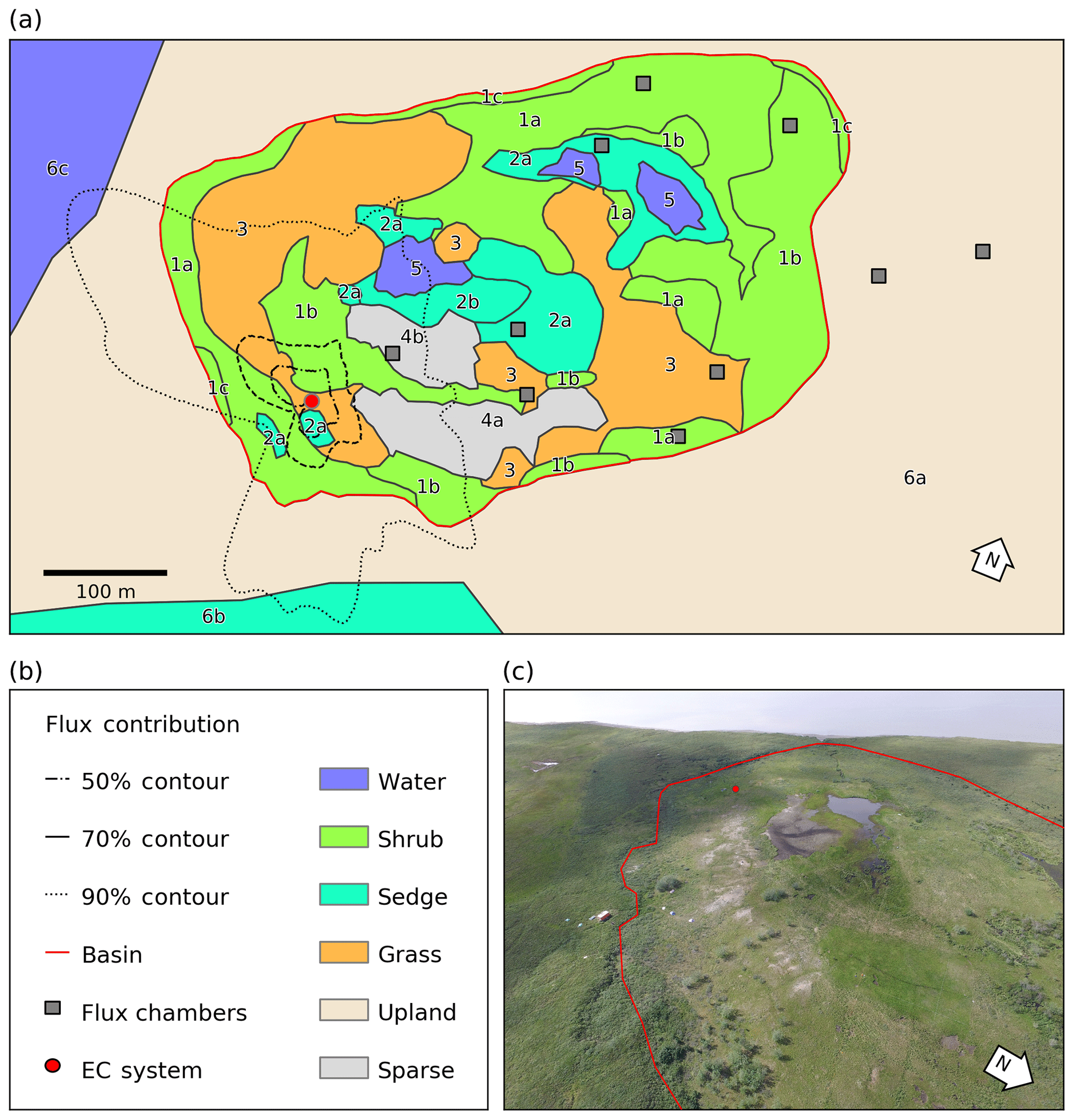
Figure 1(a) Map of the distribution of vegetation classes at Illisarvik, with the footprint climatology (FClim) over the study period, the locations of the chambers, and the eddy covariance (EC) system. The alphanumeric labels correspond to the unit codes in Table 1. (b) Legend for the map in (a). (c) Oblique drone image of Illisarvik, taken at the 16:40 23 July 2016 view from E of DTLB towards W. The basin and EC system are shown on the image using the same symbology as (a).
A vegetation survey of species composition and abundance was done on a 50 m grid in and around the basin during the 2016 study period (Wilson et al., 2019). A vegetation map was created with 10 units based on plant functional type and vegetation structure, with sub-units denoting sub-canopy vegetation. The unit boundaries between grid points were estimated visually by traversing the grid lines. Additional survey data on vegetation units and canopy height were collected manually with a GPS in the proximity of the EC station because greater resolution was needed for footprint modelling. Aerial imagery was collected on 23 July over two flights using a Phantom 2 drone (DJI, Shenzhen, China). The GPS points and drone imagery were used to cross-reference and modify the map of Wilson et al. (2019). The 10 units were then aggregated into six broader surface cover classes (listed from largest to smallest areal fraction within the footprint climatology (FClim); see Sect. 2.3 for definition): shrub, grass, sedge, upland, sparse, and water (Fig. 1 and Table 1).
2.2 Weather and soil measurements
Weather data were logged on a CR1000 data logger (Campbell Scientific Inc, Logan, UT, USA; CSI) at 5 min intervals. Net all-wave radiation (Rn) and photosynthetic photon flux density (PPFD) were measured with a NR Lite net radiometer (Kipp and Zonen, Delft, Netherlands) and a SQ-110 quantum sensor (Apogee Instruments, Logan, UT, USA), respectively, 3.2 m above the grass surface on the main EC system tripod (Fig. 1). A shielded HMP35 (CSI) recorded Ta and relative humidity (RH) 2 m above the surface. A tipping bucket rain gauge (R.M Young Company, Traverse City, MI, USA) was placed 3 m to the west of the main tripod. Soil temperature and moisture were measured within soil pits in two different vegetation types near the tripod: grass (30 m to the east) and shrub (40 m to the north). Measurements were made of ground heat flux (G) with custom-made heat flux plates, soil temperatures (Ts) with custom type-T thermocouples at depths of 0.08 m, and 0–20 cm integrated volumetric water content (VWC) with CS616 water content reflectometers (CSI). The soil measurements were recorded at 30 min intervals on CR10x data loggers (CSI). The climate and soil stations operated uninterrupted from 10 July (day 192) and 11 July (day 193), respectively, until 7 August 2016 (day 220). On 11 July and 6 August thaw depth was measured at each of the 10 chamber sites (see below). Thaw depth was measured by inserting a graduated steel probe into the ground to the point of refusal. Each site was probed five times: the median value has been used as the thaw depth at each location. On 12 and 15 July, a large herd of reindeer (∼500 animals) visited Illisarvik. They mostly avoided the tripod but did graze near it for about an hour on 12 July, which may have affected greenhouse gas fluxes.
2.3 EC fluxes
An EC system was placed in the southwestern portion of the basin (69∘28′47.82′′, −134∘35′18.6′′) and measured fluxes of CO2 () and CH4 () for the full study period between 10 July and 7 August 2016. The EC system consisted of an open-path infrared CO2∕H2O gas analyzer (IRGA) (model LI-7500, LI-COR Inc., Lincoln, NE, USA; LI-COR), an open-path CH4 analyzer (model LI-7700, LI-COR), and a CSAT3 sonic anemometer (CSI) mounted on a tripod at a measurement height (zm) of 3 m (Fig. 2). The EC data and air pressure (Pa) were logged at 10 Hz on the LI-7550 analyzer interface unit (LI-COR). The CSAT3 was oriented to the northeast (40∘) because climatology for Tuktoyaktuk indicated northerly and easterly winds are typical for July and August (Environment Canada, 2016).
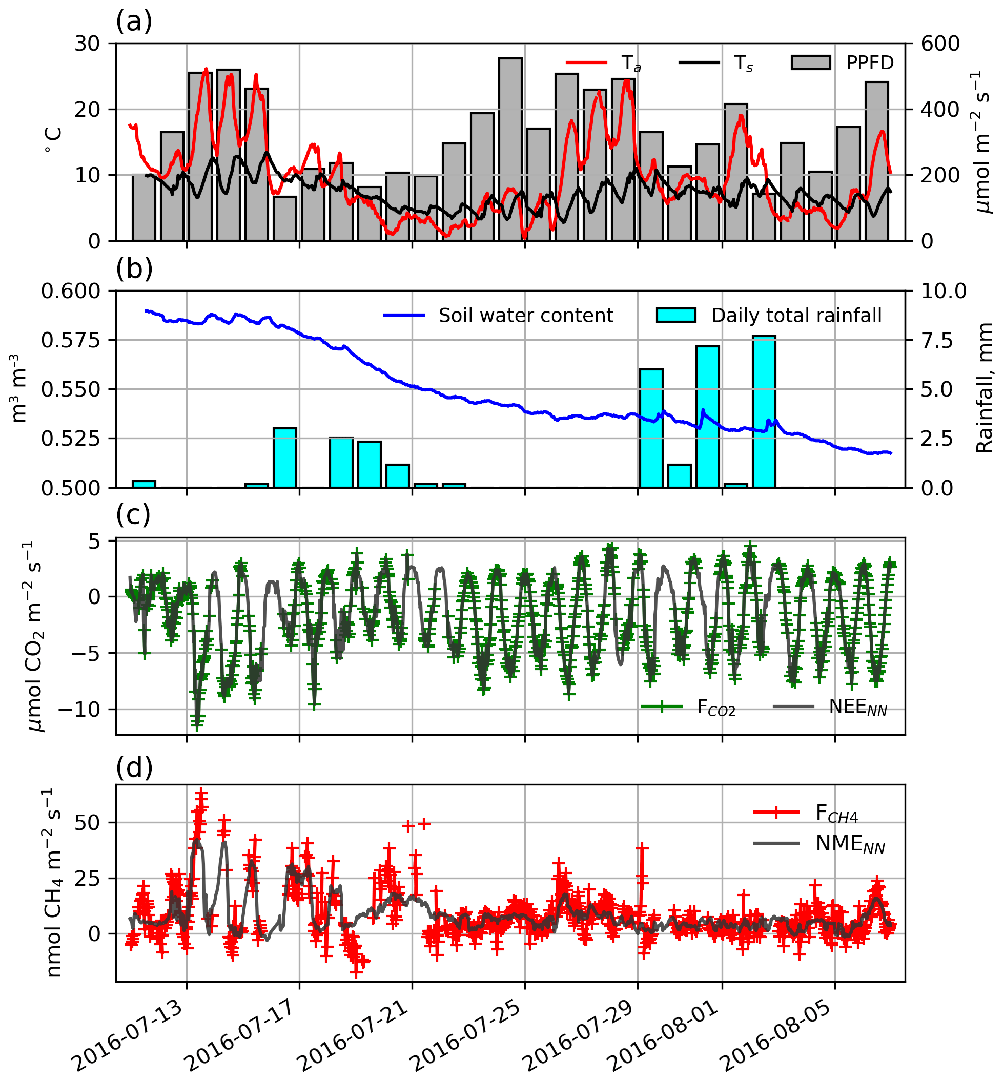
Figure 2(a) Half-hourly air and soil temperatures, displayed along with photosynthetic photon flux density (PPFD). (b) Hourly soil volumetric water content and daily total precipitation. (c) Half-hourly (green) and NEENN (grey) and (d) half-hourly (red) and NMENN (grey).
Half-hourly fluxes were calculated with EddyPro v.6.2.0 (LI-COR). The software performed statistical assessments (Vickers and Mart, 1997), performed low- and high-frequency spectral corrections (Moncrieff et al., 1997 and 2004), performed a double rotation (Wilczak et al., 2001), applied the WPL correction to account for density fluctuations (Webb et al., 1980), and computed quality control (qc) flags (Mauder and Foken, 2004). Post-processing treatments included storage correction (calculating the net flux as the sum of the observed scalar flux and the rate of change in scalar concentration at zm), filtering fluxes by friction velocities (u∗) below 0.1 m s−1, removing qc flags = 2 (Mauder and Foken, 2004), and the mean absolute deviation spike removal algorithm (Papale et al., 2006). Additionally, observations with mean winds of 220±30∘ were removed to avoid uncertainties associated with the wake of the sonic anemometer, and observations were removed during precipitation events and when the open-path analyzers indicated there were any other obstructions within the path (Aubinet et al., 2012). The data were gap-filled using neural networks (NNs) which have been applied to and in other studies (Moffat et al., 2010; Dengel et al., 2013). Details of the NN methodology are described in Appendix A.
The flux footprint represents the influence of upwind areas on a measured scalar flux, and the footprint climatology is the average of individual footprints over a time period. Evaluation of the flux footprints and climatology helps evaluate the reliability of the dataset and estimate the source area of each individual half-hourly EC flux measurement. A scalar flux Fc sampled at , where zm is the height of the EC instrumentation, can be represented as the integral of the flux footprint function f(x,y) and the distribution of sources–sinks (Qc) over a domain D (Kljun et al., 2015):
The flux contribution of upwind source areas increases sharply upwind from the measurement location to a peak and then decreases gradually with increasing distance (Schmid, 2002). The empirically derived flux footprint function of Kljun et al. (2015) was used to estimate the source area of each half-hourly flux measurement.
The model requires boundary layer heights which were not measured on site. Half-hourly boundary layer heights were interpolated from 3 h estimates obtained from the Global Data Assimilation System of the US National Oceanic and Atmospheric Administration. The model also requires the aerodynamic roughness length (z0), which is influenced by the canopy height and spacing. Canopy height (Ch) varied considerably within the basin (from >1 m in the north to ∼0 m in the bare-ground areas). Canopy height variability was lower in the vicinity of the EC tripod but ranged from 0.35 to 0.55 m with a few taller shrubs approaching 1 m. Median z0 was calculated for 30∘ wind sectors following Paul-Limoges et al. (2013). This calculation was performed for near-neutral conditions: , where L is the Obukhov length. The z0 for each wind sector was found to be insensitive to zero-plane displacement height, d, as zm≫d, so the mean value of d around the tripod was used, where . Zero-plane displacement did not change significantly over the course of the study so z0 remained fixed over the study period for each wind sector.
For each half-hourly flux observation, f(x,y)i was solved at 1 m2 resolution over a 1 km2 domain centred on the EC tripod. Then, f(x,y)i values were intersected with the surface classes to determine the relative contribution of each surface type to each flux observation (referred to as FShrub, FSedge, etc.). The footprint function is technically infinite so a fraction of each f(x,y)i was not contained within the model domain. The out-of-domain source fraction ranged from 1.8 % to 4.9 % with a mean of 3.2 % and was assumed to have minimal impact on the analysis. The flux footprint climatology (FClim) was calculated by averaging the half-hourly flux footprints over the study period and is shown in Fig. 1. Table 2 shows the flux contribution of each vegetation class.
Table 2The surface cover class fractions of the basin, along with the mean source area fractions of the footprint climatology (FClim) and the range of source area fractions for individual half-hourly observations shown in brackets.

2.4 Closed chamber measurements
In addition to EC measurements, fluxes of CO2 and CH4 were sampled using a static non-steady-state chamber flux technique on 11 dates between 12 July and 5 August 2016 (Laforce, 2018). Nineteen chamber collars were located at 10 sites, eight sites within and two outside the basin (Fig. 1). Each surface cover class was represented by at least one chamber site, except for open water. At each vegetated site a pair of collars were installed 20 cm apart, except at the “sparse” site where only one collar was installed. The above-ground biomass was removed from one of the collars at each vegetated site. There were three replicates (six collars) for the shrub class; two for the sedge; grass, and upland tundra; and no replicates for the Sparse class. PVC collars 30 cm long and 24.3 cm in diameter were inserted to a depth of approximately 15 cm. The chambers were 34 cm tall and made out of polycarbonate covered in black opaque tape to maintain dark conditions inside the chamber (for more details, see Martin et al., 2018). The chambers contained a small vent (10 cm coiled 1/8 in. diameter copper pipe) to ensure a constant pressure during measurements. The opaque chamber fluxes of CO2 provided an independent estimation of ER. This helped characterize ER given the challenges with standard NEE partitioning techniques at high-latitude sites during the Arctic summer as noted in Sect. 2.5.1.
Chamber flux measurements were made between 09:00 and 17:00 starting at a different collar set each day to randomize the sampling order to avoid a bias due to diurnal patterns. During gas flux measurements, the chambers were sealed to the top of the collars within a groove filled with water, and five 24 mL air samples were collected into evacuated 12 mL vials sealed with doubled septa. Each vial contained a small amount of magnesium perchlorate to dry the air sample. Samples were collected at 0, 5, 10, 15, and 20 min after the chambers were set on the collars. Air within the chamber was mixed with a 60 mL syringe attached to a three-way stopcock before each air sample was taken. Samples were stored until analysis 1 month later at Carleton University. The integrity of the vials through shipping, storage, and analysis was confirmed using a subset filled with helium before the field season began.
Concentrations of CO2, CH4, and N2O were determined using a CP 3800 gas chromatograph (Varian Inc., Palo Alto, CA, USA) as described by Wilson and Humphreys (2010). Three replicates of five CO2∕CH4 standards varying from 383.1 to 15 212.6 ppm CO2 and from 1.08 to 22.11 ppm CH4 were included in every set of measurements to create a linear relationship between gas concentration and chromatogram area. The chamber fluxes of CO2 and CH4 (FC) were calculated as follows:
where (dc∕dt) is the linear rate of change in the mixing ratio of the gas, A is the chamber area (0.0464 m3), V is the chamber volume (between 0.0182 and 0.0242 m3 adjusted for collar depth at each collar location), R is the ideal gas constant, P is pressure in pascals, and T is the air temperature in kelvin. P and T values corresponding to the time of each measurement were obtained from the EC station. Visual inspection of the linear trend of gas concentrations (dc∕dt) was used to identify and remove spurious point measurements associated with analysis errors, leaking chambers (isolated decreases in concentration), and contamination or ebullition events (isolated increases in concentration) (0.3 %, 0.7 %, and 2.0 % of CO2 samples and 2.1 %, 0.5 %, and 1.1 % of CH4 samples, respectively). In all flux measurements, at least three or more gas samples remained so that dc∕dt and its coefficient of determination (R2) were determined using least-squares linear regression. We did not use R2 as an additional quality control criterion as many of our CH4 fluxes were near zero and tended to have low R2 values due to only small variations in the point sample concentrations (see also Clark et al., 2020). A total of 40 % and 32 % of the 227 CH4 flux measurements and 97 % and 92 % of the 227 CO2 flux measurements had R2 over 0.80 and 0.90, respectively. No flux measurements were removed from the analysis. Positive fluxes indicate emissions of gases to the atmosphere, and negative fluxes indicate uptake by the surface.
2.4.1 Upscaling
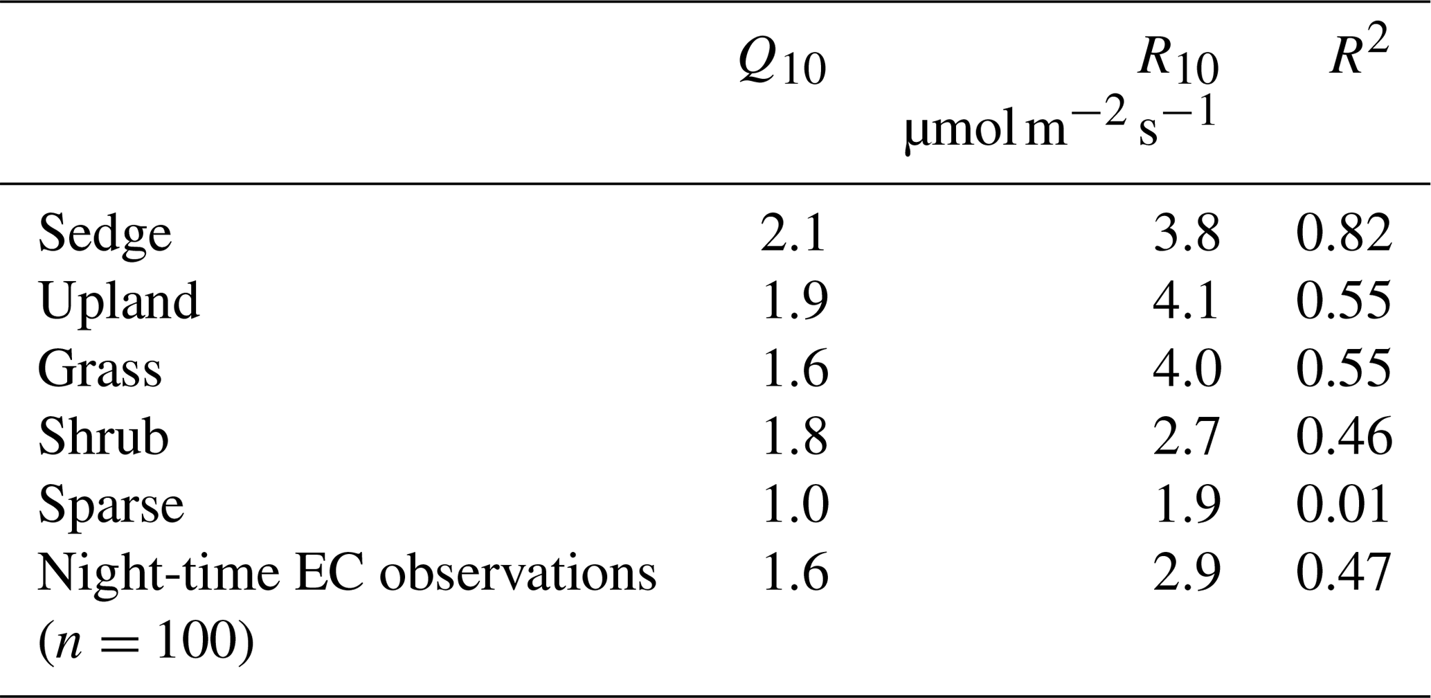
Chamber fluxes of ER were upscaled from the plot scale (individual chamber) to the footprint scale using the footprint-weighted average method and to the basin scale using the area-weighted average method (Budishchev et al., 2014). The chamber ER and air temperature from the EC tripod (Ta) were used to determine R10, the base respiration at 10 ∘C, and Q10, the temperature sensitivity coefficient, using Eq. (3) for five of the six surface classes (Fig. 1) (Laforce, 2018) (Table 3).
Half-hourly footprint-scale estimates (ERFS) were calculated by multiplying ER derived from Eq. (3) for each surface class by the footprint source area fraction and summing over classes. Basin-scale estimates (ERBS) were estimated the same way but using the mean source area fractions of the basin (Table 2). As there were no open water class ER estimates, ER from open water was assumed to be zero.
Table 3The ER temperature sensitivity (Q10) and base respiration (R10) estimated by Laforce (2018) and estimated from nighttime EC footprint observations.
In contrast to ER, there are no standard empirical functions to estimate temporal variations in NME. Instead, we used ordinary least-squares regression (OLS) to estimate NME. The most important environmental controls over were VWC and Ts (discussed below). Continuous observations of these factors at the flux chambers were not available; instead chamber NME values were grouped by vegetation class and fit to VWC and Ts measured in the soil pits near the EC station. Half-hourly footprint-scale (NMEFS) and basin-scale (NMEBS) estimates were then made using the OLS parameters for each surface class using the same procedures for ERFS and ERBS.
2.5 Factor selection and gap filling
We used an exploratory approach to identify the smallest set of factors that best predicted half-hourly EC-derived NEE and NME without overfitting the dataset using a series of neural networks (NNs). We started with 10 factors: four meteorological variables (PPFD, Ta, vapour pressure deficit (VPD) computed using the Ta and relative humidity (RH) data, and three-dimensional wind speed (U) measured using the CSAT3 sonic anemometer), two soil variables (VWC and Ts averaged between the two soil pits near the EC tripod), and four source area fractions (shrub, FShrub; grass, FShrub; sedge FSedge; and upland, FUpland). The four source area variables correspond to surface classes sampled by the chambers. We excluded water (FWater) and sparse (FSparse) fractions because its average contribution to the EC observations was only 0.2 % and 2.2 %, respectively, and there were no chamber measurements for the water class while chamber measurements indicated ER was low and NME was not significantly different from zero for the sparse class. A number of these prediction factors were highly correlated, but it was necessary to include them so the model could account for source area heterogeneity.
The NNs were trained iteratively on bootstrapped datasets. First NNs were trained on each factor individually, and the one with the lowest mean squared error (MSE) was selected. Next, NNs were trained on that factor in combination with one of the remaining nine. The best performing additional factor was again selected, and this process was repeated until MSE failed to improve. The most parsimonious model was identified using the 1 standard error (SE) rule. Dybowski and Roberts (2001) give the standard error of a bootstrap estimate of a given error metric (e.g. θ=MSE) to be
where θboot is the mean of the bootstrapped samples. The smallest set of factors where θboot was within one SEboot of the minimum θboot for both NEE and NME was selected for further analysis. The outputs from the selected models are referred to as NEENN and NMENN. NN modelling was done using the Keras Python library (Chollet et al., 2015); see Appendix A for a more detailed explanation of the NN analysis.
Multiple imputation (MI) was then used to gap-fill the NEE and NME with the NEENN and NMENN, respectively (Vitale et al., 2018). Of the 1296 half-hourly flux observations 28.9 % of and 31.3 % of were missing or filtered out. There were a few gaps in the source area fractions needed to gap-fill the flux time series because the footprint function is not valid when m s−1. When source area fractions were missing, they were gap-filled by using the mean source area fraction observed for winds within ±5∘ of the observed wind direction. The meteorological and soil data were continuous and did not need to be gap-filled.
2.5.1 Flux partitioning
NEE is negative when there is net uptake of CO2 by the ecosystem and positive when there is net emission. ER and GPP are always positive, ER represents the sum of heterotrophic and autotrophic respiration, and GPP represents photosynthetic uptake of CO2. Night-time NEE observations (e.g. PPFD≤10 ) are typically used to quantify ER because GPP is ∼0 (Aubinet et al., 2012). We fit the limited night-time EC observations available (n=95) to Eq. (3) for comparison with the ER measured using the chambers. We used the fitted values to model daytime ER and approximate NEE by fitting the daytime data to a light response curve (Aubinet et al., 2012).
Here α is the initial slope of the light response curve, β is GPP at saturation, and c is a curvature parameter. These estimates are referred to as ER and NEE.
Some NN analyses of NEE have trained separate models for night-time and daytime conditions for partitioning purposes (Papale and Valentini, 2003). However, these methods are not practical during the Arctic summer as the sun did not set at Illisarvik until 28 July, over halfway through the study period. There were not enough night-time samples to train a separate NN. Instead, we estimated ER by calculating NEENN at PPFD = 0 for all observations, henceforth referred to as ERNN. This is a projection outside of the observed parameter space resulting in greater uncertainty and a wider confidence interval around ERNN than NEENN. Calculation of confidence intervals for NN outputs is discussed in Appendix A.
2.5.2 Factor analysis
The trained NNs were used to investigate how individual factors influenced NEE and NME. The partial first derivative of the model response to one controlling factor was calculated while keeping all other inputs fixed. For example, the partial first derivative, , is an approximation of the NEE light response curve under a specific set of conditions. Similarly, NMENN can be used to approximate NME response to controls like VWC or Ts. For both fluxes, the selected models contained at least one source area fraction variable, indicating the vegetation type(s) which had significant influence over NEE and NME. Additionally, we mapped NEENN and NMENN to 100 % coverage for individual surface classes to see how fluxes at Illisarvik may change as vegetation succession continues. For example, to project to 100 % sedge coverage, we set the other surface classes to 0 % and left the other environmental factors unchanged. This allows for an estimation of how carbon fluxes may change if vegetation succession leads Illisarvik to look more like the DTLBs studied in Alaska.
During the 29 d study, half-hourly Ta and Ts ranged between 0.4 and 26.2 ∘C and 4.4 and 11.0 ∘C, respectively (Fig. 2a). Day length and maximum solar altitude decreased from 24 to 19.25 h and 41.6 to 35.4∘, but daily PPFD was more influenced by variations in cloud cover. Precipitation (19 mm) fell on 14 of the 28 d with trace snowfall on three of those days, but VWC of the soils decreased throughout the period (Fig. 2b). At the onset of the study period, VWC was high and soils were saturated with ponding in the sedge areas. By the end of the study most of this surface water had dried up. On 11 July average thaw depth (cm) was 37, 45, 51, 64, and 81 at upland, sedge, grass, shrub, and sparse classes, respectively. By 6 August, average thaw depth had increased to 45, 62, and 66 cm at upland, sedge, and grass surface classes and over 100 cm at both the shrub and sparse classes.
A strong low-pressure system stalled off the coast between day of year (DOY) 199 and 204. This caused westerly winds to occur much more frequently than is typical for July and August. The 50 %, 80 %, and 90 % flux FClim contours are shown in Fig. 1a. Mean source area fractions indicate the EC observations were skewed towards the grass surface class and under-sampled for the shrub class, but the range of surface classes sampled was diverse enough to allow for testing of the impact of source area fraction on the fluxes (Table 2).
3.1 EC observations
Half-hourly observations of and along with the NEENN and NMENN used to gap-fill the time series are shown in Fig. 2c and d. Gap-filled daily NEE ranged from −3.7 to −0.2 g C−CO2 with a mean of −1.5 [CI95 %±0.2] g C−CO2 . Day-to-day variability was considerable but there was no notable trend in NEE over the peak growing season. The half-hourly NEE during the study period reached a minimum of −10.4 just before solar noon and peaked at 4.7 around midnight (Fig. 2c). NEENN was used to gap-fill the flux data because it was in good agreement with observation (r2=0.91). Daily ERNN was estimated to be 2.2 [CI95 %±0.9] g C−CO2 with corresponding GPP of 3.7 g C−CO2 . ERNN was in poor agreement (R2=0.35, n=95) with night-time observations. For comparison, Eq. (3) provided a better fit (R2=0.47) with night-time EC data, and ER was estimated to be 3.0 g C−CO2 . However, NEE did not fit as well (r2=0.80) as NEENN.
Gap-filled daily NME was modest and decreased over the study period. It ranged from 2.0 to 25.1 mg C−CH4 with a mean of 8.7 [CI95 %±0.4] mg C−CH4 (Fig. 2d). NMENN was used to gap-fill the flux data because it provided a reasonable fit (r2=0.62) to observations. NME did not constitute a significant component of the carbon balance and thus the flux footprint area was a carbon sink during the peak growing season with negative global warming potential (GWP) after accounting for the greater GWP of CH4 (IPCC, 2104).
3.2 Chamber observations
ER was highest in the sedge, upland, and grass classes where fluxes were very similar at 5.5 [CI95 %±1.2], 5.4 [CI95 %±1.2], and 4.9 [CI95 %±0.7] g C−CO2 . Shrub ER was significantly less (3.5 [CI95 %±0.6] g C−CO2 ) than the other vegetated classes, and sparse ER was the lowest among the classes (2.0 [CI95 %±0.3] g C−CO2 ) (Fig. 3a). The Q10 and R10 values also differed between vegetation classes: ER in the sedge class was the most sensitive to changes in air temperature, and modelled values provided the best fit (R2=0.82) to observations. Upland and grass had the highest base respiration and fit observations moderately well (Table 3).
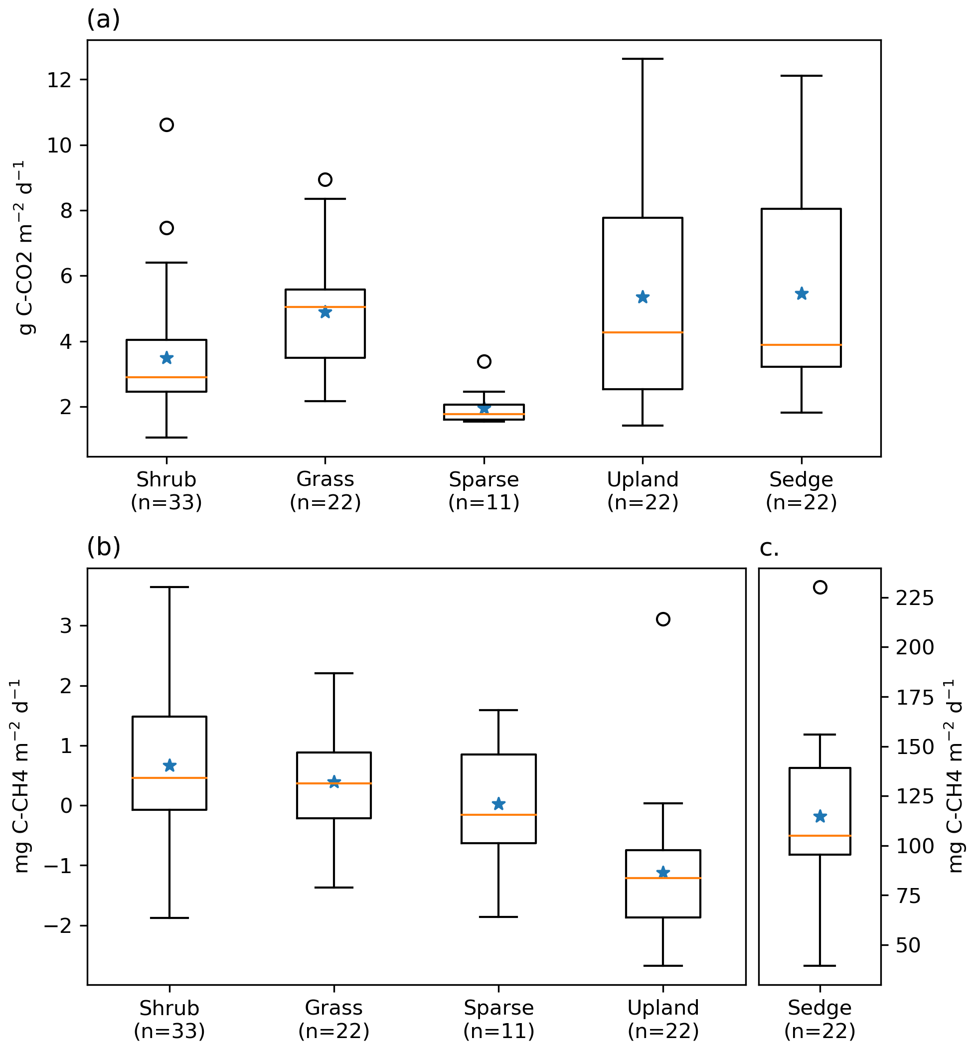
Figure 3Box plot of (a) ER, (b) NME, and (c) NME fluxes measured using closed chambers, grouped by vegetation class. The orange lines represent the median, blue stars represent means, the boxes indicate the interquartile range (Q1–Q3), the whiskers indicate and ), and the circles represent outliers extending beyond the whiskers. Note the scale for (c) sedge is different.
NME was more variable between vegetation classes than ER (Fig. 3b and c). Sedge was a very strong CH4 source at 114.7 [CI95 %±15.3] mg C−CH4 . Shrub and grass were very weak sources, 0.7 [CI95 %±0.3] and 0.4 [CI95 %±0.3] mg C−CH4 , respectively. Sparse was neutral. Upland was a net CH4 sink −1.1 [CI95 %±0.4] mg C−CH4 . Sedge and shrub NME values were positively correlated with Ts (r=0.61, p<0.01; r=0.35, p=0.04) and VWC (r=0.58, p<0.01; r=0.5, <0.01). They also had a positive correlation with Ta, while upland NME was negatively correlated with Ta. Grass and sparse did not have any significant correlations.
Footprint-scaled chamber fluxes were 59 % and 47 % higher than ERNN or gap-filled NME, respectively. Mean ERFS was 3.5 g C−CO2 [CI95 %±0.1], it fit ER very well (R2=0.95) as would be expected and ERNN moderately well (R2=0.46). Mean NMEFS was 12.8 [CI95 %±1.3] mg C−CH4 ; it did not fit NMENN well (R2=0.30). At the basin scale, ERBS (3.4 [CI95 %±0.1] g C−CO2 ) was slightly lower than ERFS because of the exclusion of upland areas. NMEBS was higher (15.2 [CI95 %±0.1] g C−CO2 ) because of the greater sedge fraction in the basin than the footprint (Table 2).
3.3 NEE response to environmental factors and vegetation type
NEENN (r2=0.91) was estimated using four factors: PPFD, VPD, VWC, and FShrub. PPFD is the primary control over NEE: a NN trained on PPFD alone provided a reasonable fit (r2=0.83). The three additional factors, VPD, VWC, and FShrub, helped NEENN fit a wider variety of conditions. Examining the partial first derivative of NEENN under different conditions provides interpretation of the modelled light response curves (Fig. 4). The minimum values represent the peak light use efficiency and are analogous to α in Eq. (5) (Fig. 4b). With increasing PPFD, light use becomes less efficient and approaches zeros as the light response nears light saturation (Fig. 4b).
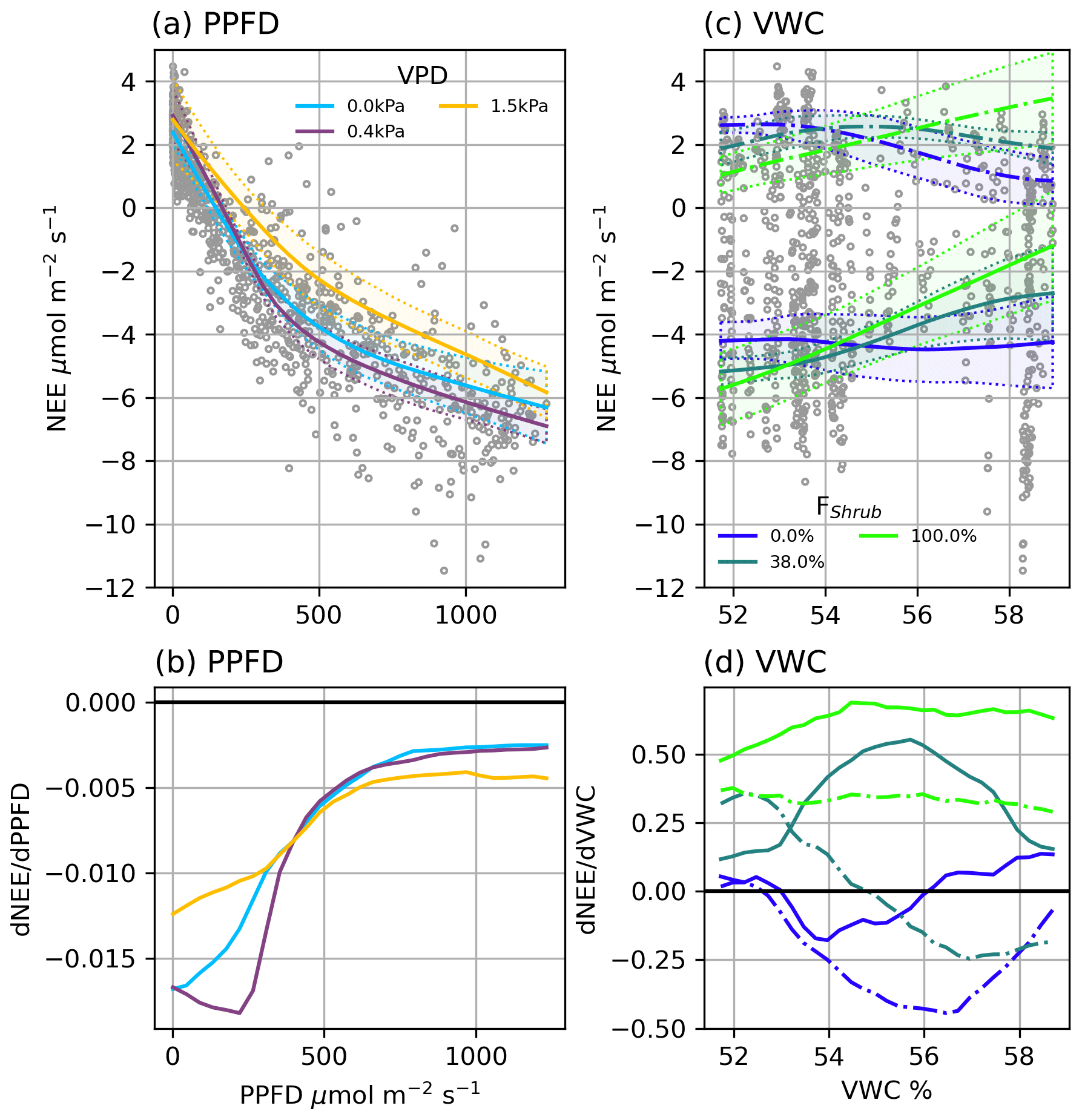
Figure 4(a) Modelled NEE response to PPFD under different VPD conditions and (b) the partial first derivatives of NEE with respect to PPFD. (c) Modelled ER (dashed line) and NEE (solid line) response to VWC at different Shrub% values and (d) the partial first derivatives of ER (dashed lined) and NEE (solid line) with respect to VWC. NEE in (c) was calculated at PPFD = 600 µmol m2 s−1. The shaded areas in (a) and (c) are 95 % confidence intervals and grey circles are the EC observations.
VPD was a secondary control over NEE. Increasing VPD increased peak light use efficiency and net CO2 uptake until a threshold, above which it had a strong limiting effect (Fig. 4a and b). For example, under dry atmospheric conditions (e.g. VPD = 1.5 kPa), peak light use is less efficient (−12 nmol CO2 µmol−1 photon) than under more humid conditions (−18 nmol CO2 µmol−1 photon). The value of this VPD threshold was dependent upon soil moisture: from 1 kPa when VWC was highest to 0.25 Pa when VWC was low. Mapping NEENN and ERNN at FShrub=100 %, FShrub=0 %, and FShrub=36 % (FClim) shows that VWC and FShrub were the primary controls over ER and thus influenced NEE (Fig. 4c and d). We can see from the partial first derivates of NEENN that increasing VWC increases ER from shrub areas. In the absence of shrubs, increasing VWC inhibits ER, although it is important to note that variations in VWC were subtle, ranging from 51.7 % to 59.0 %. The partial first derivative of NEENN shows that VWC slightly limits NEE from non-shrub areas and significantly reduces it in shrub areas.
3.4 NME response to environmental factors and vegetation type
NMENN (r2=0.62) was estimated using five factors: FSedge, FShrub, VWC, TS, and U. NME was more variable and less dependent on any one factor than NEE, which is why the NMENN needed an extra factor and had a lower r2 score. The source area had a significant effect on NME, and it was encouraging that the model contained FSedge and FShrub since sedge and shrub were the strongest CH4 source and largest footprint component, respectively. These two factors can combine to map NME under three general situations: we can extrapolate to FSedge=100 % and FShrub=0 % or FSedge=0 % and FShrub=100 %, or we can represent actual FClim, where FSedge=11 % and FShrub=37 % (Table 2). Some upland tundra was included in theFClim estimate, which reduced NME.

Figure 5(a) Modelled NME response to VWC at different source area fractions and (b) the partial first derivatives of NME with respect to VWC. (c) Modelled NME response to Ts at different source area fractions and (d) the partial first derivatives of NME with respect to Ts. The shaded areas in (a) and (c) are 95 % confidence intervals and grey circles are the EC observations.
VWC was the primary climatic driver identified by NMENN. Wetter soils had a consistent positive effect on NME, which was strongest when FSedgewas high (Fig. 5a and b). Between the driest and wettest conditions, estimated NME increased: by an order of magnitude at FSedge=100 %, 4-fold at FShrub=100 %, and from neutral to a source at FClim (Fig. 5a). Higher Ts generally had a negative effect on NME (Fig. 5c and d). The negative correlation between Ts and VWC (r=0.54, <0.01) may have contributed to this result. NMENN performance improved less with the addition of U, indicating the NMENN was near saturation and its effects are less relevant. Higher U had a weak limiting effect on NME when VWC was high and increased NME when VWC was low (not shown).
4.1 Carbon balance and controlling factors
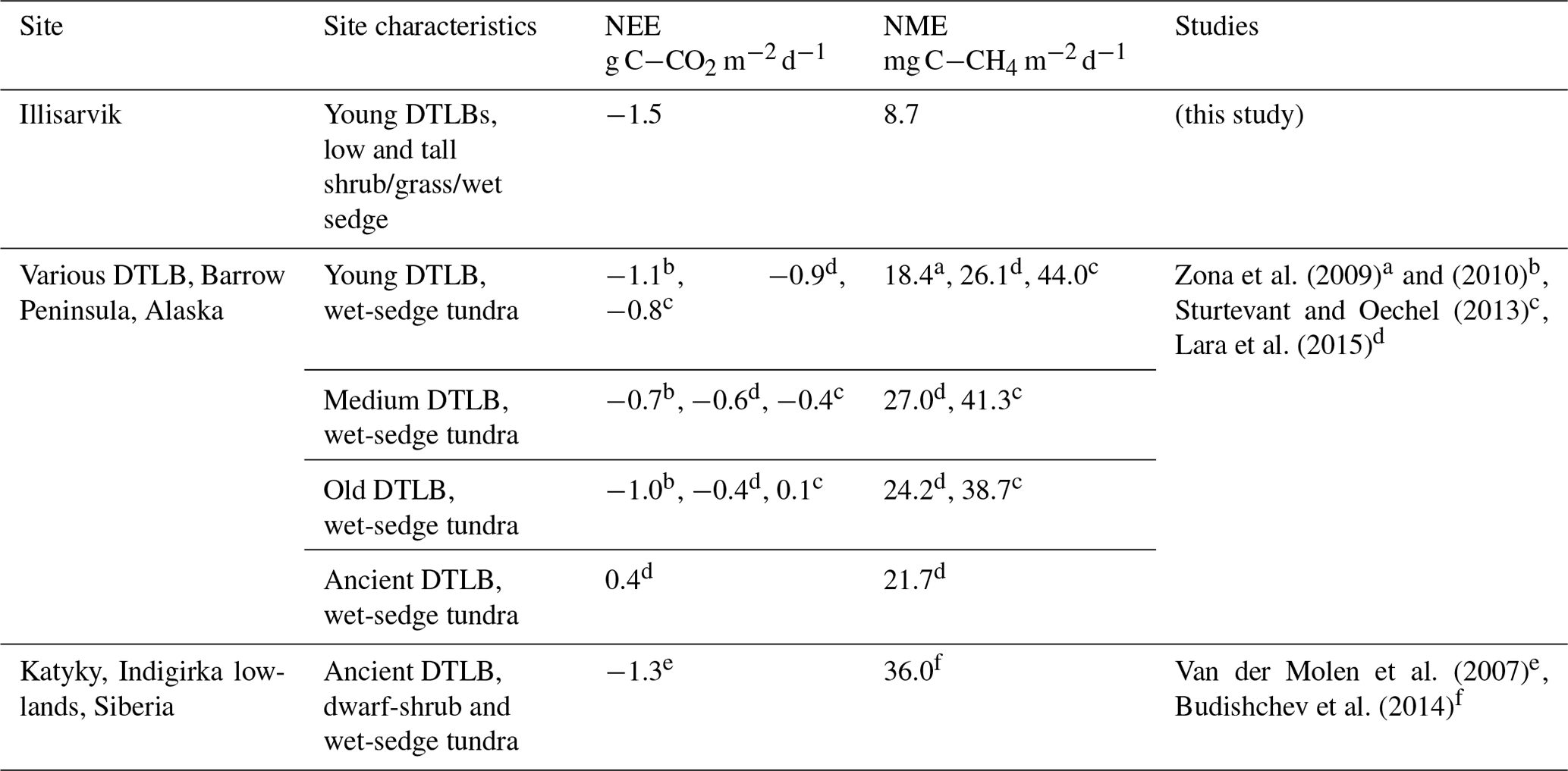
Compared to other DTLBs, Illisarvik has drier soils and greater shrub and grass cover (Table 4). Peak growing season CO2 uptake at Illisarvik was greater than at most wet-sedge-dominated DTLBs (Table 4; Zona et al., 2010, Sturtevant and Oechel, 2013; Lara et al., 2015). These differences may be due to differences in the periods of observation and year-to-year variability but may also be due to the presence of more productive shrubs and slightly warmer climate at Illisarvik. Mean 1980–2010 Ta at Utqiaġvik (formerly Barrow, AK) is −11.2 ∘C (US National Climate Data Centre, 2020). Tuktoyaktuk, the closest station to Illisarvik, is 1.1∘ warmer. Shrub cover is expected to have a number of impacts on the microclimate and carbon cycle of Arctic tundra (e.g. Myers-Smith et al., 2011). Typically, greater deciduous shrub cover is expected to increase GPP as a result of greater leaf area and photosynthetic potential compared to graminoid-dominated tundra (Sweet et al., 2015; Street et al., 2018). GPP was greater at Illisarvik compared to the young wet-sedge-dominated DTLBs in Alaska (Zona et al., 2010). It was more similar to Katyk, which has significant dwarf-shrub cover, predominately Betula nana and Salix pulchra (van der Molen et al., 2007).
Table 4Growing season (gs) daily range in eddy-covariance-derived NEE and NME from drained thermokarst lake basins (DTLBs) and other select wetland and coastal tundra sites across the Arctic.
The periods of study
measurements for the study observations are as follows.
a Mid-June–end of July.
b 12 June–28 August 2007, Fig. 4.
c 11 June–25 August 2011.
d Upscaled
chamber estimates, exact dates not specified.
e Mean 15 June–31 August 2003–2006.
f 5 July–4 August 2009.
Differences in ER among tundra environments can be related to substrate availability, soil moisture and temperature, and thaw depth, among other factors (Sturtevant and Oechel, 2013). The “snow-shrub hypothesis” (Sturm et al., 2001) describes the potential for greater snow trapping in shrub communities which insulates soils in winter, leads to increased decomposition and nutrient availability, and promotes further shrub growth. At Illisarvik, snow blowing in off the Arctic Ocean results in large snow drifts within the basin where snow depth correlates with vegetation height (Wilson et al., 2019). Wilson et al. (2019) concluded that the soils within the Illisarvik basin were warmer than those of the surrounding dwarf-shrub tundra in part through these snow–shrub interactions. Although our chamber observations suggested shrub ER is lower than ER from other vegetation classes, this may have been an artifact as the taller shrubs (>40 cm) could not fit inside the chambers. In another study, chamber ER increased with greater shrub cover in upland tundra (Ge et al., 2017). ER at Illisarvik was greater than the ER observed at both the young wet-sedge DTLB in Barrow (Zona et al., 2010) and at the shrub–wet-sedge DTLB at Katyk where thaw depth was much shallower (45 to >100 cm at Illisarvik vs. 25 to 40 cm at Katyk; van der Molen et al., 2007). The importance of FShrub in describing temporal variations in half-hourly NEE within the flux footprint at Illisarvik is further evidence of the importance of shrub cover on tundra carbon cycle processes in this environment.
PPFD and VPD were the most important factors for predicting half-hourly NEE. This was to be expected as they are typically the primary controls over GPP (Aubinet et al., 2012). The limiting effects of VPD are consistent with another study using NN to analyze NEE at a deciduous forest site (Moffat et al., 2010) and have been found at other tundra sites (Euskirchen et al., 2012; López-Blanco et al., 2017). VWC was also important at Illisarvik. Zona et al. (2010) found VWC could explain 70 % of the variability in daily peak season ER in a young DTLB. Similarly, Kittler et al. (2016) found drier soils increased ER and decreased NEE after a wet tundra drainage experiment in Siberia, consistent with our results at Illisarvik when FShrub was low.
As expected, NME at Illisarvik was about half that observed at the Alaskan DTLB sites where soils were wetter with greater sedge cover (Table 4, Zona et al., 2009; Lara et al., 2015). NME at Katyk was even higher than the Barrow DTLBs and had a significant impact on the greenhouse gas (GHG) balance for this site (van der Molen et al., 2007; Parmentier et al., 2011). In our NN modelling of NME at Illisarvik, FSedge was the most important factor for predicting half-hourly . Sedges are aquatic plant species with aerenchymatous tissues that act as conduits for CH4 from below the water table to the atmosphere and limit CH4 oxidation by methanotrophs in aerobic surface soils (Lai et al., 2009). The inclusion of FShrub further refined the model, allowing it to better fit the site-specific distribution of vegetation types. Budishchev et al. (2014) found shrub and sedge fraction had a significant influence on at Katyk. Vegetation type is the dominant control over NME across multiple tundra landscapes and our results further support that (Davidson et al., 2016).
VWC was the second most important factor, which was expected as CH4 production occurs in anaerobic environments and has been linked to variability in CH4 emission in many other studies (e.g. Zona et al., 2009; Nadeau et al., 2013; Olefeldt et al., 2013). Soil temperature (Ts) was the third most important factor. Higher Ts values increase the oxidation potential of methanotrophs (Liu et al., 2016; King and Adamsen, 1992), so this result was expected for the drier portions of the basin and upland tundra. However, this was not expected for the sedge areas because most studies find NME in sedges is positively correlated to Ts (Olefeldt et al., 2013). The negative correlation between Ts and VWC may partly explain this.
4.2 Upscaling
ERFS and NMEFS were about 59 % and 47 % greater than the gap-filled EC estimates. Discrepancies between EC and chamber observations are common and have been attributed to differences in measurement techniques, the small sample size of chamber observations, and sampling bias since all chamber measurements were taken during the day with fair weather (Katayanagi et al., 2005; Chaichana et al., 2018). Meijide et al. (2011) found that chamber NEE could be up to twice as large as EC observations, and Riederer et al. (2014) also found chamber NME estimates were about 30 % higher than EC estimates. Others have been more successful, yielding upscaled chamber NME fluxes within 10 % of EC observations (Zhang et al., 2012; Budishchev et al., 2014; Davidson et al., 2017). A potential reason for the disagreement with ERFS may be the lack of direct observations by the EC system under low-light conditions. Another potential source of error for the upscaling is inaccuracies in the vegetation map.
4.3 Future trajectories
Presently, peak growing season carbon uptake at Illisarvik is greater than similarly aged landscape features on the Barrow Peninsula, Alaska, and more similar to levels observed at Katyk, Siberia. NME is well below levels observed at any other DTLB studied, making this site a stronger GHG sink than other DTLBs. However, the basin at Illisarvik will continue to evolve, and the trajectory it takes could significantly alter its carbon balance. Historically, DTLBs on Richards Island and the Tuktoyaktuk Peninsula evolve into sedge wetlands, as do DTLBs on the Barrow Peninsula (Ovendend, 1986; Lara et al., 2015). Active maintenance of the outlet channel at Illisarvik has artificially lowered soil moisture and flooding and potentially limited this transition thus far (C. Burn, personal communication, 2016).
If Illisarvik follows the same trajectory as older DTLBs in the area and becomes dominated by sedge wetlands, NME will increase significantly. Figure 5a shows that with extrapolations to full sedge cover (FSedge=100 %), NME would be similar to values on the Barrow Peninsula (Zona et al., 2009). If the basin instead transitions into a shrub-dominated DTLB similar to those of Old Crow Flats, Yukon (Lantz and Turner, 2015), NMENN would remain similar to current levels, meaning the basin would remain a weak source of CH4. These are projections well beyond FClim fractions observed, so confidence in the specific values predicted is low.
The effects of changing shrub and sedge cover on Illisarvik's growing season NEE are less straightforward than on NME, partly because shrub cover had less overall influence on NEENN. Figure 4c shows that the model suggests ER decreases and NEE increases with increasing shrub coverage when soils are slightly drier but has the opposite effect under wetter conditions. To our knowledge, only a few winter season (e.g. Zona et al., 2016) and no year-round studies of DTLB NEE and NME have been published to help evaluate the factors influencing carbon losses through the non-growing-season months. Further observation year-round is needed to better understand the implications of continued vegetation change for the carbon balance of DTLBs such as Illisarvik.
This study investigated NEE, GPP, ER, and NME in the Illisarvik experimental DTLB using EC and chamber data. To our knowledge this is the first such study conducted in a DTLB outside of the Barrow Peninsula or Siberia. Illisarvik is a carbon sink during the growing season with NME only having a small effect on the net carbon balance. Our flux observations were generally in agreement with other studies but show how shrub-dominated DTLBs such as Illisarvik and Katyk in Siberia differ from sedge-dominated DTLBs on the Barrow Peninsula. Illisarvik's growing season net carbon uptake was greater than young and ancient DTLBs on the Barrow Peninsula and more similar to the shrub-dominated ancient DTLB in Siberia. NME at Illisarvik was lower than all published DTLB studies, likely due to better drainage and more diverse vegetation. A longer, more comprehensive study would be needed to resolve the annual carbon budget for Illisarvik.
Chamber measurements of ER and NME from different land cover classes within and outside the Illisarvik basin added context to the EC observations. Vegetation class (and associated difference in terrain and soil properties) had only a small but significant impact on NEE and ER but was one of the dominant controls over NME. Sedge areas were a strong source of CH4, other vegetation types in the basin were weak sources, and upland areas were a net sink. These results suggest that NME in particular will change as the Illisarvik DTLB vegetation communities continue to evolve.
Typically, NEE is gap-filled using flux-partitioning algorithms that model ER and GPP separately using TS and PPFD, respectively (e.g. Lee et al., 2017; Aubinet et al., 2012). However, this method requires night-time observations and thus does not perform well for Arctic summertime measurements due to the limited number of samples available during low-light conditions. There are no widely agreed upon functional relationships for gap-filling NME since CH4 production and consumption vary considerably between both different land cover types and environmental conditions. Some methods that have been used include general linear models (GLMs) (Zona et al., 2009), mean diurnal variation (Nadeau et al., 2013), and classification and regression trees (CARTs) (Nadeau et al., 2013; Sachs et al., 2008). We attempted to use a GLM and CART but they were not flexible enough to account for source area variability.
Neural networks (NNs) are flexible machine-learning methods that are ideally suited to perform non-linear, multivariate regression. They make no a priori assumptions about the functional relationships between the factors and responses (Melesse and Hanley, 2005; Desai et al., 2008). NNs are universal approximators; given enough hidden nodes a NN is capable of mapping any continuous function to an arbitrary degree of accuracy (Hornik, 1991). If all relevant climate and ecosystem information is available to a network, the remaining variability can be attributed to noise in the measurement (Moffat et al., 2010).
NNs have been shown to be among the best performing methods for gap-filling NEE data for temperate forest and wetland sites (Papale and Valentini, 2003; Moffat et al., 2007; Knox et al., 2016). They have also been used to gap-fill NME time series in sub-Arctic wetlands, tundra sites, and wet-sedge tundra (Dengel et al., 2013). NNs have been used to identify and model factors influencing NEE and to partition NEE into ER and GPP (Moffat et al., 2010). NNs have even been used to upscale fluxes from the ecosystem level to the continental scale (Dou and Yang, 2018; Papale et al., 2003).
A NN approximates a true regression function F(X):
where t(X) is the target function and ε(X) the noise (Khosravi et al., 2011). , where x0=1 is a bias term and represents the independent variables. M denotes the number of independent variables. The network approximates F(X) as f(X,w) by mapping the relationship between X and the target. Here we used feed-forward dense NNs with a single hidden layer:
g(⋅) is a non-linear transfer function; here we used the rectified linear activation unit (ReLu) (Anders and Korn, 1999). H denotes the number of hidden nodes in the network and must be assigned before training. Too many hidden nodes and the NN will overfit the training data, too few and it will underfit. Early stopping will prevent NNs from overfitting training sets (Weigend and Lebaron, 1994; Tetko et al., 1995). Therefore, it is more important to ensure a NN has enough hidden nodes to adequately map the target function (Smith, 1993). We set H to a function of M, the number of targets (1), the number of training samples (N), and a scaling parameter (a) which was set to 2:
This rule of thumb ensures a NN has sufficient flexibility to approximate the target response. The weights are randomly initialized and after each model iteration are updated by back-propagating the error through the network. N denotes the number of observations or targets. The error metric most commonly used is the mean squared error, MSE:
The weights are adjusted in the direction that will decrease the error, and training continues until a stopping criterion is reached. We chose to set aside 20 % of the training data as a test set to be used for early stopping, and we terminated training when the MSE of the test set failed to improve for 10 consecutive iterations.
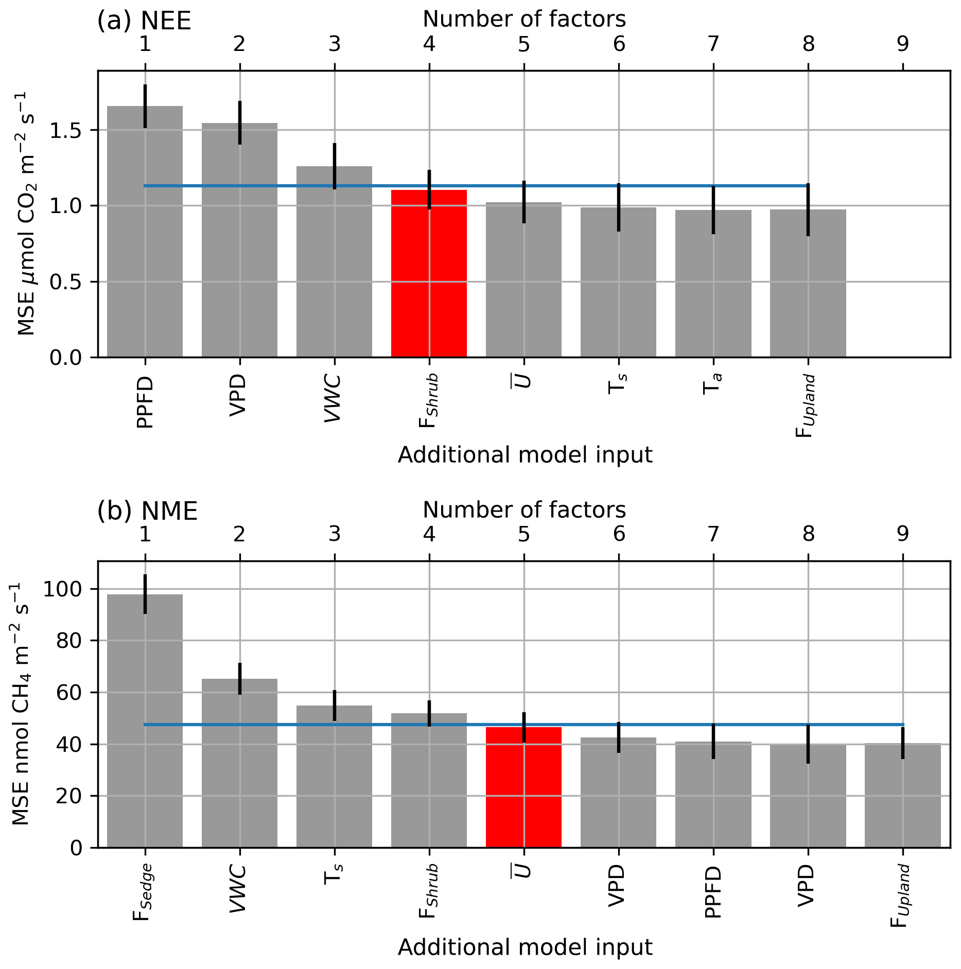
Figure A1The averaged mean squared error (θ) of the bootstrapped neural network model validation datasets, with error bars showing 1 standard error (SE). The x axis shows models of increasing size from left to right (one to nine factors), and the label indicates the factor added to the model at each step. The blue line indicates the 1 SE rule threshold, and the red bar indicates the model selected by the 1 SE rule.
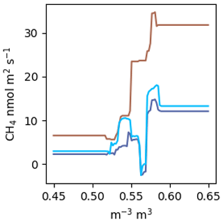
Figure A2 estimated by a RF using the same factors as the NN model. The colours correspond to the scenarios in Fig. 5a. VWC was estimated over the range from 0.45 to 0.65.
Bootstrapping is used to account for model variability and estimate confidence and prediction intervals by training NNs on B different realizations of the dataset, where B is the number of bootstrapped samples, we used B=30 (Heskes, 1997; Khosravi et al., 2011). An individual NN generates point outputs approximating a target function with no information on the confidence in those estimates (Khosravi et al., 2011). However, there are usually multiple f(X,w) values that approximate F(X) because of the random weight initializations (Weigend and LeBaron, 1994). As such, there are two sources of error we are concerned with, the accuracy of our estimation of F(X) and the accuracy of our estimates with respect to the target. A confidence interval describes the first (e.g. while a prediction interval describes the latter (e.g. (Heskes, 1997). By definition, a prediction interval contains the confidence interval because
For b=1…B, a random sample with replacement of size p is drawn from the original dataset. Setting p equal to the size of the original dataset yields a set of B training sets each containing approximately 67 % of the original dataset. The 33 % leftover from each bootstrap sampled can be used for model validation (Heskes, 1997). The average of our ensemble of networks can then serve as our approximation of F(X):
The variance of the model outputs is
A confidence interval (CI) for F(X) can be calculated as , where t is the Student t score, 1-α is the desired confidence level, and df is the degrees of freedom which are set to the number of bootstrapped samples B. NN performance can be seen to improve with the inclusion of more factors, until the model saturates and becomes over-parameterized (Fig. A1).
Random forests (RFs) are said to be among the best performing gap-filling methods for NME (Kim et al., 2020), and it has been claimed that aggregating many regression trees in a RF prevents overfitting (Breiman, 2001). We did not find this to be the case. Following the methods outlined in Kim et al. (2020): a RF with 400 trees and no restrictions on tree size fit nearly perfectly (R2=0.98). Without considerable limitations on tree size, the RF will just learn the dataset rather than the relationships present. It is our view that this tree is extremely overfit, as highlighted by the example in Fig. A2. Further, RFs do not allow for straightforward visualization functional relationships in a dataset. Plotting against VWC, which is the dominant environmental control identified, does not reveal a meaningful relationship like Fig. 5a and c. You can look at an individual decision tree within the RF, but those are difficult to interpret beyond the first few splits, and each tree will be different. Lastly, RFs are incapable of projecting beyond the parameter space observed, which limited their applicability for this study (Fig. A2). This presents an issue because many gaps in EC data arise from data filtering (e.g. clear calm nights, precipitation events) and are by definition outside the parameter space observed.
Our data and code are available on GitHub: https://github.com/June-Spaceboots/Illisarvik_CFluxes (Skeeter, 2019).
JS, AC, and GH designed the EC study. AL and EH designed the chamber study. JS collected, processed, and analyzed the EC data. AL and EH collected the chamber data with help from JS. AL and EH processed the chamber data. JS designed and conducted the NN analysis. JS prepared the manuscript with input from all co-authors.
The authors declare that they have no conflict of interest.
Funding was provided by the Canada Foundation of Innovation and the Natural Sciences and Engineering Research Council (NSERC) of Canada. Additional logistical support was provided by the Polar Continental Shelf Program, Natural Resources Canada.
This research has been supported by the Canada Foundation for Innovation – IF 2015 (grant no. 33600), NSERC Discovery Grants Program (grant no. RGPIN-2017-03958), NSERC Discovery Grants – Northern Research Supplement (grant no. RGPNS-503529), and NSERC Discovery Grants Program – Accelerator Supplement (grant no. RGPAS-507854).
This paper was edited by Lutz Merbold and reviewed by Norbert Pirk and one anonymous referee.
Anders, U. and Korn, O.: Model selection in neural networks, Neural Networks, 12, 309–323, https://doi.org/10.1016/S0893-6080(98)00117-8, 1999.
Aubinet, M., Vesala, T., and Papale, D. (Eds.): Eddy Covariance: A Practical Guide to Measurement and Data Analysis, 2012 edition, Springer, Dordrecht, New York., 2012.
Biasi, C., Meyer, H., Rusalimova, O., Hämmerle, R., Kaiser, C., Baranyi, C., Daims, H., Lashchinsky, N., Barsukov, P., and Richter, A.: Initial effects of experimental warming on carbon exchange rates, plant growth and microbial dynamics of a lichen-rich dwarf shrub tundra in Siberia, Plant Soil, 307, 191–205, https://doi.org/10.1007/s11104-008-9596-2, 2008.
Billings, W. and Peterson, K.: Vegetational Change and Ice-Wedge Polygons Through the Thaw-Lake Cycle, Arc. Antarct. Alp. Res., 12, 413–432, https://doi.org/10.2307/1550492, 1980.
Breiman, L.: Random forests, Mach. Learn., 45, 5–32, 2001.
Budishchev, A., Mi, Y., van Huissteden, J., Belelli-Marchesini, L., Schaepman-Strub, G., Parmentier, F. J. W., Fratini, G., Gallagher, A., Maximov, T. C., and Dolman, A. J.: Evaluation of a plot-scale methane emission model using eddy covariance observations and footprint modelling, Biogeosciences, 11, 4651–4664, https://doi.org/10.5194/bg-11-4651-2014, 2014.
Cahoon, S. M. P., Sullivan, P. F., Shaver, G. R., Welker, J. M., and Post, E.: Interactions among shrub cover and the soil microclimate may determine future Arctic carbon budgets, Ecol. Lett., 15, 1415–1422, https://doi.org/10.1111/j.1461-0248.2012.01865.x, 2012.
Chaichana, N., Bellingrath-Kimura, S. D., Komiya, S., Fujii, Y., Noborio, K., Dietrich, O., and Pakoktom, T.: Comparison of Closed Chamber and Eddy Covariance Methods to Improve the Understanding of Methane Fluxes from Rice Paddy Fields in Japan, Atmosphere, 9, 356, https://doi.org/10.3390/atmos9090356, 2018.
Chollet, F., Rahman, F., Lee, T., et al.: Keras, available at: https://keras.io (last access: 2 September 2020), 2015.
Clark, M. G., Humphreys, E. R., and Carey, S. K.: Low methane emissions from a boreal wetland constructed on oil sand mine tailings, Biogeosciences, 17, 667–682, https://doi.org/10.5194/bg-17-667-2020, 2020.
Davidson, S. J., Sloan, V. L., Phoenix, G. K., Wagner, R., Fisher, J. P., Oechel, W. C., and Zona, D.: Vegetation Type Dominates the Spatial Variability in CH4 Emissions Across Multiple Arctic Tundra Landscapes, Ecosystems, 19, 1116–1132, https://doi.org/10.1007/s10021-016-9991-0, 2016.
Davidson, S. J., Santos, M. J., Sloan, V. L., Reuss-Schmidt, K., Phoenix, G. K., Oechel, W. C., and Zona, D.: Upscaling CH4 Fluxes Using High-Resolution Imagery in Arctic Tundra Ecosystems, Remote Sens.-Basel, 9, 1227, https://doi.org/10.3390/rs9121227, 2017.
Dengel, S., Zona, D., Sachs, T., Aurela, M., Jammet, M., Parmentier, F. J. W., Oechel, W., and Vesala, T.: Testing the applicability of neural networks as a gap-filling method using CH4 flux data from high latitude wetlands, Biogeosciences, 10, 8185–8200, https://doi.org/10.5194/bg-10-8185-2013, 2013.
Desai, A. R., Richardson, A. D., Moffat, A. M., Kattge, J., Hollinger, D. Y., Barr, A., Falge, E., Noormets, A., Papale, D., Reichstein, M., and Stauch, V. J.: Cross-site evaluation of eddy covariance GPP and RE decomposition techniques, Agr. Forest Meteorol., 148, 821–838, https://doi.org/10.1016/j.agrformet.2007.11.012, 2008.
Dou, X. and Yang, Y.: Estimating forest carbon fluxes using four different data-driven techniques based on long-term eddy covariance measurements: Model comparison and evaluation, Sci. Total Environ., 627, 78–94, https://doi.org/10.1016/j.scitotenv.2018.01.202, 2018.
Dybowski, R. and Roberts, S. J.: Confidence intervals and prediction intervals for feedforward neural networks, in: Clinical Applications of Artificial Neural Networks, edited by: Dybowski, R. and Gant, V., Cambridge University Press, Cambridge, 298–326, 2001.
Environment Canada: Climate Data Online, available at: https://climate.weather.gc.ca/historical_data/search_historic_data_e.html (last access: 2 September 2020), 2016.
Euskirchen, E. S., Bret-Harte, M. S., Scott, G. J., Edgar, C., and Shaver, G. R.: Seasonal patterns of carbon dioxide and water fluxes in three representative tundra ecosystems in northern Alaska, Ecosphere, 3, art4, https://doi.org/10.1890/ES11-00202.1, 2012.
French, H. M.: Thermokarst Processes and Landforms, in: The Periglacial Environment 4e, John Wiley & Sons, Ltd, Oxford, 169–192, 2017.
Heskes, T.: Practical Confidence and Prediction Intervals, in: Advances in Neural Information Processing Systems, MIT press, Cambridge, 176–182, 1997.
Ge, L., Lafleur, P. M., and Humphreys, E. R.: Respiration from Soil and Ground Cover Vegetation Under Tundra Shrubs, available at: https://pubag.nal.usda.gov/catalog/5943221 (last access: 28 April 2020), 2017.
Hornik, K.: Approximation capabilities of multilayer feedforward networks, Neural Networks, 4, 251–257, 1991.
Intergovernmental Panel on Climate Change (IPCC): Climate Change 2014: Synthesis Report, Fifth Assessment Report of the Intergovernmental Panel on Climate Change, IPCC, Geneva, Switzerland, 2014..
Jones, B. M., Grosse, G., Arp, C. D., Jones, M. C., Anthony, K. M. W., and Romanovsky, V. E.: Modern thermokarst lake dynamics in the continuous permafrost zone, northern Seward Peninsula, Alaska, J. Geophys. Res.-Biogeo., https://doi.org/10.1029/2011JG001666, 2018.
Katayanagi, N.: Spatial variability of greenhouse gas fluxes from soils of various land uses on a livestock farm in southern Hokkaido, Japan, Phyton, 45, 309–318, 2005.
Khosravi, A., Nahavandi, S., Creighton, D., and Atiya, A. F.: Comprehensive Review of Neural Network-Based Prediction Intervals and New Advances, IEEE Transactions on Neural Networks, 22, 1341–1356, https://doi.org/10.1109/TNN.2011.2162110, 2011.
Kim, Y., Johnson, M. S., Knox, S. H., Black, T. A., Dalmagro, H. J., Kang, M., Kim, J., and Baldocchi, D.: Gap-filling approaches for eddy covariance methane fluxes: A comparison of three machine learning algorithms and a traditional method with principal component analysis, Glob. Change Biol., 26, 1499–1518, https://doi.org/10.1111/gcb.14845, 2020.
King, G. M. and Adamsen, A. P. S.: Effects of Temperature on Methane Consumption in a Forest Soil and in Pure Cultures of the Methanotroph Methylomonas rubra, Appl. Environ. Microbiol., 58, 2758–2763, 1992.
Kittler, F., Burjack, I., Corradi, C. A. R., Heimann, M., Kolle, O., Merbold, L., Zimov, N., Zimov, S., and Göckede, M.: Impacts of a decadal drainage disturbance on surface-atmosphere fluxes of carbon dioxide in a permafrost ecosystem, Biogeosciences, 13, 5315–5332, https://doi.org/10.5194/bg-13-5315-2016, 2016.
Kljun, N., Calanca, P., Rotach, M. W., and Schmid, H. P.: A simple two-dimensional parameterisation for Flux Footprint Prediction (FFP), Geosci. Model Dev., 8, 3695–3713, https://doi.org/10.5194/gmd-8-3695-2015, 2015.
Knox, S. H., Matthes, J. H., Sturtevant, C., Oikawa, P. Y., Verfaillie, J., and Baldocchi, D.: Biophysical controls on interannual variability in ecosystem-scale CO2 and CH4 exchange in a California rice paddy, J. Geophys. Res.-Biogeo., 121, 978–1001, https://doi.org/10.1002/2015JG003247, 2016.
Lafleur, P. M., Humphreys, E. R., St. Louis, V. L., Myklebust, M. C., Papakyriakou, T., Poissant, L., Barker, J. D., Pilote, M., and Swystun, K. A.: Variation in Peak Growing Season Net Ecosystem Production Across the Canadian Arctic, Environ. Sci. Technol., 46, 7971–7977, https://doi.org/10.1021/es300500m, 2012.
Laforce, A.-A.: Spatial variability of carbon emissions within a drained lake basin and its surrounding tundra, Illisarvik, Northwest Territories, Carleton University, 2018.
Lai, D. Y. F.: Methane Dynamics in Northern Peatlands: A Review, Pedosphere, 19, 409–421, 2009.
Lantz, T. C. and Turner, K. W.: Changes in lake area in response to thermokarst processes and climate in Old Crow Flats, Yukon, J. Geophys. Res.-Biogeo., 120, 513–524, https://doi.org/10.1002/2014JG002744, 2015.
Lara, M. J., McGuire, A. D., Euskirchen, E. S., Tweedie, C. E., Hinkel, K. M., Skurikhin, A. N., Romanovsky, V. E., Grosse, G., Bolton, W. R., and Genet, H.: Polygonal tundra geomorphological change in response to warming alters future CO2 and CH4 flux on the Barrow Peninsula, Glob. Change Biol., 21, 1634–1651, https://doi.org/10.1111/gcb.12757, 2015.
Lee, S.-C., Christen, A., Black, A. T., Johnson, M. S., Jassal, R. S., Ketler, R., Nesic, Z., and Merkens, M.: Annual greenhouse gas budget for a bog ecosystem undergoing restoration by rewetting, Biogeosciences, 14, 2799–2814, https://doi.org/10.5194/bg-14-2799-2017, 2017.
Liu, Y., Liu, X., Cheng, K., Li, L., Zhang, X., Zheng, J., Zheng, J., and Pan, G.: Responses of Methanogenic and Methanotrophic Communities to Elevated Atmospheric CO2 and Temperature in a Paddy Field, Front. Microbiol., 7, 1895, https://doi.org/10.3389/fmicb.2016.01895, 2016.
López-Blanco, E., Lund, M., Williams, M., Tamstorf, M. P., Westergaard-Nielsen, A., Exbrayat, J.-F., Hansen, B. U., and Christensen, T. R.: Exchange of CO2 in Arctic tundra: impacts of meteorological variations and biological disturbance, Biogeosciences, 14, 4467–4483, https://doi.org/10.5194/bg-14-4467-2017, 2017.
Mackay, J. R.: A full-scale field experiment (1978–1995) on the growth of permafrost by means of lake drainage, western Arctic coast: a discussion of the method and some results, Can. J. Earth Sci., 34, 17–33, https://doi.org/10.1139/e17-002, 1997.
Mackay, J. R.: Periglacial features developed on the exposed lake bottoms of seven lakes that drained rapidly after 1950, Tuktoyaktuk Peninsula area, western Arctic coast, Canada, Permafrost Periglac., 10, 39–63, https://doi.org/10.1002/(SICI)1099-1530(199901/03)10:1{<}39::AID-PPP305{>}3.3.CO;2-I, 1999.
Mackay, J. R. and Burn, C. R.: The first 20 years (1978–1979 to 1998–1999) of active-layer development, Illisarvik experimental drained lake site, western Arctic coast, Canada, Can. J. Earth Sci., 39, 1657–1674, https://doi.org/10.1139/E02-068, 2002.
Marsh, P., Russell, M., Pohl, S., Haywood, H., and Onclin, C.: Changes in thaw lake drainage in the Western Canadian Arctic from 1950 to 2000, Hydrol. Process., 23, 145–158, https://doi.org/10.1002/hyp.7179, 2009.
Martin, A. F., Lantz, T. C., and Humphreys, E. R.: Ice wedge degradation and CO2 and CH4 emissions in the Tuktoyaktuk Coastlands, Northwest Territories, Arct. Sci., 4, 130–145, 2018.
Mauder, M. and Foken, T.: Documentation and Instruction Manual of the Eddy Covariance Software Package TK2, Univ. Bayreuth Abt. Mikrometeorologie, Bayreuth, 2004.
McGuire, A. D., Anderson, L. G., Christensen, T. R., Dallimore, S., Guo, L., Hayes, D. J., Heimann, M., Lorenson, T. D., Macdonald, R. W., and Roulet, N.: Sensitivity of the carbon cycle in the Arctic to climate change, Ecol. Monogr., 79, 523–555, https://doi.org/10.1890/08-2025.1, 2009.
Meijide, A., Manca, G., Goded, I., Magliulo, V., di Tommasi, P., Seufert, G., and Cescatti, A.: Seasonal trends and environmental controls of methane emissions in a rice paddy field in Northern Italy, Biogeosciences, 8, 3809–3821, https://doi.org/10.5194/bg-8-3809-2011, 2011.
Melesse, A. M. and Hanley, R. S.: Artificial neural network application for multi-ecosystem carbon flux simulation, Ecol. Model., 189, 305–314, https://doi.org/10.1016/j.ecolmodel.2005.03.014, 2005.
Michel, F. A., Fritz, P., and Drimmie, R. J.: Evidence of climatic change from oxygen and carbon isotope variations in sediments of a small arctic lake, Canada, J. Quaternary Sci., 4, 201–209, https://doi.org/10.1002/jqs.3390040302, 1989.
Moffat, A. M., Papale, D., Reichstein, M., Hollinger, D. Y., Richardson, A. D., Barr, A. G., Beckstein, C., Braswell, B. H., Churkina, G., Desai, A. R., Falge, E., Gove, J. H., Heimann, M., Hui, D., Jarvis, A. J., Kattge, J., Noormets, A., and Stauch, V. J.: Comprehensive comparison of gap-filling techniques for eddy covariance net carbon fluxes, Agr. Forest Meteorol., 147, 209–232, https://doi.org/10.1016/j.agrformet.2007.08.011, 2007.
Moffat, A. M., Beckstein, C., Churkina, G., Mund, M., and Heimann, M.: Characterization of ecosystem responses to climatic controls using artificial neural networks, Glob, Change Biol,, 16, 2737–2749, https://doi.org/10.1111/j.1365-2486.2010.02171.x, 2010.
Moncrieff, J., Clement, R., Finnigan, J., and Meyers, T.: Averaging, Detrending, and Filtering of Eddy Covariance Time Series, in: Handbook of Micrometeorology, edited by: Lee, X., Massman, W., and Law, B., Springer Netherlands, 7–31, 2004.
Moncrieff, J. B., Massheder, J. M., de Bruin, H., Elbers, J., Friborg, T., Heusinkveld, B., Kabat, P., Scott, S., Soegaard, H., and Verhoef, A.: A system to measure surface fluxes of momentum, sensible heat, water vapour and carbon dioxide, J. Hydrol., 188, 589–611, https://doi.org/10.1016/S0022-1694(96)03194-0, 1997.
Myers-Smith, I. H., Forbes, B. C., Wilmking, M., Hallinger, M., Lantz, T., Blok, D., Tape, K. D., Macias-Fauria, M., Sass-Klaassen, U., Lévesque, E., Boudreau, S., Ropars, P., Hermanutz, L., Trant, A., Collier, L. S., Weijers, S., Rozema, J., Rayback, S. A., Schmidt, N. M., Schaepman-Strub, G., Wipf, S., Rixen, C., Ménard, C. B., Venn, S., Goetz, S., Andreu-Hayles, L., Elmendorf, S., Ravolainen, V., Welker, J., Grogan, P., Epstein, H. E., and Hik, D. S.: Shrub expansion in tundra ecosystems: dynamics, impacts and research priorities, Environ. Res. Lett., 6, 045509, https://doi.org/10.1088/1748-9326/6/4/045509, 2011.
Nadeau, D. F., Rousseau, A. N., Coursolle, C., Margolis, H. A., and Parlange, M. B.: Summer methane fluxes from a boreal bog in northern Quebec, Canada, using eddy covariance measurements, Atmos. Environ., 81, 464–474, https://doi.org/10.1016/j.atmosenv.2013.09.044, 2013.
Olefeldt, D., Turetsky, M. R., Crill, P. M., and McGuire, A. D.: Environmental and physical controls on northern terrestrial methane emissions across permafrost zones, Glob. Change Biol., 19, 589–603, https://doi.org/10.1111/gcb.12071, 2013.
O'Neill, H. B. and Burn, C. R.: Physical and temporal factors controlling the development of near-surface ground ice at Illisarvik, western Arctic coast, Canada, Can. J. Earth Sci., 49, 1096–1110, 2012.
Ovenden, L.: Vegetation Colonizing the Bed of a Recently Drained Thermokarst Lake (illisarvik), Northwest-Territories, Can. J. Bot., 64, 2688–2692, 1986.
Papale, D. and Valentini, R.: A new assessment of European forests carbon exchanges by eddy fluxes and artificial neural network spatialization, Glob. Change Biol., 9, 525–535, https://doi.org/10.1046/j.1365-2486.2003.00609.x, 2003.
Papale, D., Reichstein, M., Aubinet, M., Canfora, E., Bernhofer, C., Kutsch, W., Longdoz, B., Rambal, S., Valentini, R., Vesala, T., and Yakir, D.: Towards a standardized processing of Net Ecosystem Exchange measured with eddy covariance technique: algorithms and uncertainty estimation, Biogeosciences, 3, 571–583, https://doi.org/10.5194/bg-3-571-2006, 2006.
Parmentier, F. J. W., van Huissteden, J., van der Molen, M. K., Schaepman-Strub, G., Karsanaev, S. A., Maximov, T. C., and Dolman, A. J.: Spatial and temporal dynamics in eddy covariance observations of methane fluxes at a tundra site in northeastern Siberia, J. Geophys. Res.-Biogeo., 116, G3, https://doi.org/10.1029/2010JG001637, 2011.
Paul-Limoges, E., Christen, A., Coops, N., Black, T., and Trofymow, J.: Estimation of aerodynamic roughness of a harvested Douglas-fir forest using airborne LiDAR, Remote Sens. Environ., 136, 225–233, https://doi.org/10.1016/j.rse.2013.05.007, 2013.
Riederer, M., Serafimovich, A., and Foken, T.: Net ecosystem CO2 exchange measurements by the closed chamber method and the eddy covariance technique and their dependence on atmospheric conditions, Atmos. Meas. Tech., 7, 1057–1064, https://doi.org/10.5194/amt-7-1057-2014, 2014.
Sachs, T., Wille, C., Boike, J., and Kutzbach, L.: Environmental controls on ecosystem-scale CH4 emission from polygonal tundra in the Lena River Delta, Siberia, J. Geophys. Res.-Biogeo., 113, G00A03, https://doi.org/10.1029/2007JG000505, 2008.
Schmid, H. P.: Footprint modeling for vegetation atmosphere exchange studies: a review and perspective, Agr. Forest Meteorol., 113, 159–183, https://doi.org/10.1016/S0168-1923(02)00107-7, 2002.
Skeeter, J.: June-Spaceboots/Illisarvik_CFluxes, available at: https://github.com/June-Spaceboots/Illisarvik_CFluxes, last access: 3 December 2019.
Street, L. E., Subke, J.-A., Baxter, R., Dinsmore, K. J., Knoblauch, C., and Wookey, P. A.: Ecosystem carbon dynamics differ between tundra shrub types in the western Canadian Arctic, Environ. Res. Lett., 13, 084014, https://doi.org/10.1088/1748-9326/aad363, 2018.
Sturm, M., Racine, C., and Tape, K.: Increasing shrub abundance in the Arctic, Nature, 411, 546–547, https://doi.org/10.1038/35079180, 2001.
Sturtevant, C. S. and Oechel, W. C.: Spatial variation in landscape-level CO2 and CH4 fluxes from arctic coastal tundra: influence from vegetation, wetness, and the thaw lake cycle, Glob. Change Biol., 19, 2853–2866, https://doi.org/10.1111/gcb.12247, 2013.
Sweet, S. K., Griffin, K. L., Steltzer, H., Gough, L., and Boelman, N. T.: Greater deciduous shrub abundance extends tundra peak season and increases modeled net CO2 uptake, Glob. Change Biol., 21, 2394–2409, https://doi.org/10.1111/gcb.12852, 2015.
Tarnocai, C., Canadell, J. G., Schuur, E. A. G., Kuhry, P., Mazhitova, G., and Zimov, S.: Soil organic carbon pools in the northern circumpolar permafrost region: Soil organic carbon pools, Global Biogeochem. Cy., 23, 1–11, https://doi.org/10.1029/2008GB003327, 2009.
Tetko, I. V., Livingstone, D. J., and Luik, A. I.: Neural network studies. 1. Comparison of overfitting and overtraining, J. Chem. Inf. Model., 35, 826–833, https://doi.org/10.1021/ci00027a006, 1995.
van der Molen, M. K., Huissteden, J. van, Parmentier, F. J. W., Petrescu, A. M. R., Dolman, A. J., Maximov, T. C., Kononov, A. V., Karsanaev, S. V., and Suzdalov, D. A.: The growing season greenhouse gas balance of a continental tundra site in the Indigirka lowlands, NE Siberia, Biogeosciences, 4, 985–1003, https://doi.org/10.5194/bg-4-985-2007, 2007.
van Huissteden, J., Berrittella, C., Parmentier, F. J. W., Mi, Y., Maximov, T. C., and Dolman, A. J.: Methane emissions from permafrost thaw lakes limited by lake drainage, Nat. Clim. Change, 1, 119–123, https://doi.org/10.1038/nclimate1101, 2011.
Vickers, D. and Mahrt, L.: Quality Control and Flux Sampling Problems for Tower and Aircraft Data, J. Atmos. Oceanic Technol., 14, 512–526, https://doi.org/10.1175/1520-0426(1997)014<0512:QCAFSP>2.0.CO;2, 1997.
Virkkala, A.-M., Virtanen, T., Lehtonen, A., Rinne, J., and Luoto, M.: The current state of CO2 flux chamber studies in the Arctic tundra: A review, Prog. Phys. Geog., 42, 030913331774578, https://doi.org/10.1177/0309133317745784, 2018.
Vitale, D., Bilancia, M., and Papale, D.: A Multiple Imputation Strategy for Eddy Covariance Data, J. Environ. Inform., 34, 68–87, 2018.
Walker, D., Raynolds, M., Daniëls, F., Einarsson, E., Elvebakk, A., Gould, W., Katenin, A., Kholod, S., Markon, C., Melnikov, E., Moskalenko, N., Talbot, S., Yurtsev, B., and Team, T.: The Circumpolar Arctic Vegetation Map, J. Veg. Sci., 16, 267–282, https://doi.org/10.1111/j.1654-1103.2005.tb02365.x, 2005.
Walter, K. M., Smith, L. C., and Chapin, F. S.: Methane Bubbling from Northern Lakes: Present and Future Contributions to the Global Methane Budget, Philosophical Transactions: Mathematical, Phys. Eng. Sci., 365, 1657–1676, 2007.
Webb, E., Pearman, G., and Leuning, R.: Correction of Flux Measurements for Density Effects Due to Heat and Water-Vapor Transfer, Q. J. Roy. Meteor. Soc., 106, 85–100, https://doi.org/10.1002/qj.49710644707, 1980.
Weigend, A. S. and Lebaron, B.: Evaluating Neural Network Predictors by Bootstrapping, Humboldt University of Berlin, Interdisciplinary Research Project 373: Quantification and Simulation of Economic Processes, available at: https://ideas.repec.org/p/zbw/sfb373/199435.html (last access: 21 January 2019), 1994.
Whalen, S. C. and Reeburgh, W. S.: Consumption of atmospheric methane by tundra soils, Nature, 346, 160–162, https://doi.org/10.1038/346160a0, 1990.
Wilczak, J. M., Oncley, S. P., and Stage, S. A.: Sonic Anemometer Tilt Correction Algorithms, Bound.-Lay. Meteorol., 99, 127–150, https://doi.org/10.1023/A:1018966204465, 2001.
Wilson, M. A., Burn C. R., and Humphreys E. R.: Vegetation Development and Variation in Near-Surface Ground Temperatures at Illisarvik, Western Arctic Coast, Cold Regions Engineering 2019, 687–695, https://doi.org/10.1061/9780784482599.079, 2019.
Wilson, K. S. and Humphreys, E. R.: Carbon dioxide and methane fluxes from arctic mudboils, Can. J. Soil Sci., 90, 441–449, https://doi.org/10.4141/CJSS09073, 2010.
Zhang, Y., Sachs, T., Li, C., and Boike, J.: Upscaling methane fluxes from closed chambers to eddy covariance based on a permafrost biogeochemistry integrated model, Glob. Change Biol., 18, 1428–1440, https://doi.org/10.1111/j.1365-2486.2011.02587.x, 2012.
Zona, D., Oechel, W. C., Kochendorfer, J., Paw U, K. T., Salyuk, A. N., Olivas, P. C., Oberbauer, S. F., and Lipson, D. A.: Methane fluxes during the initiation of a large-scale water table manipulation experiment in the Alaskan Arctic tundra, Glob. Biogeochem. Cy., 23, GB2013, https://doi.org/10.1029/2009GB003487, 2009.
Zona, D., Oechel, W. C., Peterson, K. M., Clements, R. J., Paw, U. K. T., and Ustin, S. L.: Characterization of the carbon fluxes of a vegetated drained lake basin chronosequence on the Alaskan Arctic Coastal Plain, Glob. Change Biol., 16, 1870–1882, https://doi.org/10.1111/j.1365-2486.2009.02107.x, 2010.
Zona, D., Lipson, D. A., Paw U, K. T., Oberbauer, S. F., Olivas, P., Gioli, B., and Oechel, W. C.: Increased CO2 loss from vegetated drained lake tundra ecosystems due to flooding, Glob. Biogeochem. Cy., 26, GB2004, https://doi.org/10.1029/2011GB004037, 2012.
Zona, D., Gioli, B., Commane, R., Lindaas, J., Wofsy, S. C., Miller, C. E., Dinardo, S. J., Dengel, S., Sweeney, C., Karion, A., Chang, R. Y.-W., Henderson, J. M., Murphy, P. C., Goodrich, J. P., Moreaux, V., Liljedahl, A., Watts, J. D., Kimball, J. S., Lipson, D. A., and Oechel, W. C.: Cold season emissions dominate the Arctic tundra methane budget, P. Natl. Acad. Sci. USA, 113, 40–45, https://doi.org/10.1073/pnas.1516017113, 2016.
Zulueta, R. C., Oechel, W. C., Loescher, H. W., Lawrence, W. T., and Paw U. K. T.: Aircraft-derived regional scale CO2 fluxes from vegetated drained thaw-lake basins and interstitial tundra on the Arctic Coastal Plain of Alaska, Glob. Change Biol., 17, 2781–2802, https://doi.org/10.1111/j.1365-2486.2011.02433.x, 2011.