Mapping the Sensitivity of Population Exposure to Changes in Flood Magnitude: Prospective Application From Local to Global Scale

Introduction

Floods are a substantial threat to societies around the world, hampering sustainable development (UNISDR, 2015). Especially in developing countries, flood events are a key factor that can push additional people into poverty (Winsemius et al., 2018). Moreover, floods are expected to become more frequent in several regions as a result of climatic changes (IPCC, 2012). Hence, flooding and flood risk have become major topics for investigation in both the disaster risk and the climate change impact research community. The scale and spatial resolution are crucial for studying floods and their impacts (Kundzewicz et al., 2019). Studying floods on a global scale requires different approaches than studying floods on a local or regional scale. Modeling floods on a global scale requires the use of simplified models on a coarse spatial and temporal scale and is often based on several assumptions that are used to parametrize the effects of local-scale processes (Ward et al., 2015). In contrast, modeling floods on a local scale requires specific data and high spatial resolution (Bermúdez and Zischg, 2018). However, cross-scale issues arise when studying the impact of climatic change on floods and flood risk (Mateo et al., 2017; Fleischmann et al., 2019), meaning that techniques for downscaling or disaggregation are required. Global climate models (GCMs) provide the basis for flood models, but the outputs of these models need to be downscaled to continental or regional scales with regional climate models (RCMs) and then coupled with regional- and local-scale hydrological and inundation models to provide flood projections (Gusyev et al., 2016; Felder et al., 2018). In these approaches, simulations of river flows are run continuously over a selected period, and the resulting flood events are analyzed using extreme value statistics. Examples of this type of modeling approach are given in IPCC (2012), Pappenberger et al. (2012), Hirabayashi et al. (2013), Ward et al. (2013), Dottori et al. (2018), Winsemius et al. (2018). These models provide global information concerning the regions in which river flow and thus flooding is likely to increase or decrease. Several recent studies analyzing these changes in flood risk have included more drivers of change, such as an increase in population or economic growth. For example, Jongman et al. (2012), Winsemius et al. (2015), Güneralp et al. (2015), Kinoshita et al. (2017), and Aerts et al. (2018) consider the future spatiotemporal patterns of settlements and socio-economic activities in their model cascades.

However, the use of model cascades that are driven by global and RCMs is controversial. The precipitation output of a GCM/RCM model cascade often exhibits significant biases (Smith et al., 2014; Felder et al., 2018), and methods to correct these biases are therefore required (Prudhomme et al., 2002). Thus, uncertainties can occur in model cascades as a result of the climate model structure selected and the choice of technique used for downscaling and correction (Prudhomme et al., 2010; Cloke et al., 2013; Steinschneider et al., 2015a). Moreover, the results of these models have been found to be sensitive to climate forcing and the structure of the GCM used (Ward et al., 2013), resulting in uncertainties that also propagate through the coupled hydrologic and hydraulic models (Steinschneider et al., 2015b; Trigg et al., 2016; Grimaldi et al., 2019). Significant uncertainties are also associated with return period estimates under current and future climatic conditions (Winsemius et al., 2013), depending on the length of observation and the periods simulated, and thus on the sample size used for extreme value statistics (Smith et al., 2014; Trigg et al., 2016). Hence, the capacity of this approach to identify and analyze extreme flood events is still under discussion (Felder et al., 2018).

To overcome the uncertainties and problems associated with model cascades, alternative approaches are currently being developed (Guo et al., 2017; Knighton et al., 2017; Kim et al., 2018; Broderick et al., 2019; Keller et al., 2019a; Keller et al., 2019b). In studies investigating the impacts of climate change on hydrology, a scenario-neutral approach has been used to analyze the sensitivity of river flows to changes in temperature and precipitation, where the observed rainfall and temperature data are modified by stepwise increases or decreases in the value of associated parameters. The disturbed data are then fed into a hydrological model, and the resulting changes in river flow are analyzed in relation to the changes in the atmospheric parameters. Another approach to analyze the sensitivity of flood impacts to changing environmental conditions is based on downward counterfactual analysis (Aspinall and Woo, 2019; Woo, 2019). According to Roese (1997), a downward counterfactual is a thought about the past in which the outcome is worse than what actually happened. The concept of counterfactual thinking initially comes from cognitive psychology (Roese and Olson, 1995) and is used in natural hazard research to extend the range of possible hazard events. The exploration of alternative (worse) realizations of past hazardous events is used to extend knowledge concerning the impact of rare extreme events. If applied in flood risk analyses, an extreme meteorological event is perturbed and alternative, physically plausible scenarios of the same event are modeled. The impacts of the counterfactual outcomes are analyzed and compared with the impacts of the observed event; for example, the consequences of a hypothetical deviation of the observed track of a storm or an increase in rainfall (Staffler et al., 2008; Guo et al., 2016).

This allows to answer questions as, for example, “What if the rainfall event had been 10% more intense?” The artificial worsening of a historic flood event by computer simulations is similar to sensitivity analysis in model experiments, but the selection of the changes to be analyzed differs. Conventional sensitivity analysis makes “blind” changes in both directions (increases and decreases in the input parameters) within specified limits, which can lead to higher or lower impacts. In downward counterfactual analysis, the range over which the vulnerability of a system is tested is driven by searching for different future, plausible scenarios in which flood impacts will increase. The scenarios considered in downward counterfactual analysis are thus a subset of scenarios of a sensitivity analysis. Given the large uncertainty associated with projections of future climate change, such analyses typically encompass a wide range of possible futures.

Despite the growing interest in flood risk analyses under changing climate conditions, an explicit method for mapping the sensitivity of flood exposure or risk estimates to climatic changes is currently lacking. Hence, the main aim of this paper is to develop and evaluate a generalized method that can be used to analyze the sensitivity of floodplains to changes in the magnitude of floods in terms of exposure. In terms of exposure, we focus on population. Thus, exposure here is defined as the absolute number of population potentially affected by a specific flood scenario. Furthermore, we present the possible application of this method to fluvial floods at various spatial scales. However, the examples presented below can also be used as a blueprint for analyzing the exposure of other categories, such as infrastructure and assets.

Materials and Data

The method used for mapping the sensitivity of population exposure to changes in the magnitude of floods consists of performing a geographical overlay of flood hazard maps with population data. We focus on riverine floods and do not consider coastal floods or the flooding of small mountain rivers. Datasets are available from which the proposed method can be applied without the need for purposefully performing flood simulations. The main requirements are datasets that include both flood maps and information about the population in the area investigated. The flood maps and population datasets are then brought to the same spatial resolution. Flood maps with a coarse resolution compared to the population maps can be downscaled by a water volume distribution approach and projected onto a digital elevation model with a higher spatial resolution following the procedure by Winsemius et al. (2015). Coarse population data can be downscaled and disaggregated to the spatial resolution of the flood hazard maps according to the procedures outlined in Stevens et al. (2015), Calka et al. (2017), Lloyd et al. (2017), and Tatem (2017).

Flood Hazard Maps

Flood hazard maps are usually based on regional flood frequency approaches. Flood flows are estimated from pooled river gauged data (Trigg et al., 2016) and upstream catchment characteristics (Sampson et al., 2015), or regional hydrologic simulations (UNISDR, 2015). These approaches represent the present day frequency of river flooding. In general, flood hazard maps with specific return periods (or exceedance probabilities) are modeled, using periods such as 10, 20, 50, 100, 200, 500, or 1,000 years.

The application of this method on the local scale is based on hydraulic simulations and synthetic hydrographs describing a wide range of flood magnitudes. The synthetic hydrographs were derived from the analysis of typical flood events and typical shapes of hydrographs and flood peak-volume relationships were extracted from historic flood events to be used for scaling the flood magnitude as outlined in Zischg et al. (2018a) and Zischg et al. (2018c). The synthetic hydrographs with increasing flood magnitudes were subsequently used to elaborate a set of inundation maps that can be overlaid with population data. This allows the analysis of the relationship between flood magnitude and exposure.

Detailed maps of flood prone areas are available on a national scale for many countries. In order to test the proposed method at this scale, data from the National Mapping System for Floodable Zones (Sistema Nacional de Cartografía de Zonas Inundables, hereafter SNCZI) was used, which includes information for return periods of 10, 50, 100, and 500 years (MARM, 2011). These maps were developed by the Spanish Ministry of Ecological Transition and are freely available on the SNCZI website. The maps combine information obtained from historical flood records, hydrological-hydraulic studies, and geomorphological analyses.

Flood maps from the Joint Research Centre of the European Commission JRC (Alfieri et al., 2016; Dottori et al., 2016; Dottori et al., 2018) were used to test the applicability of the method on a global scale. Flood scenarios with return periods of 10, 20, 50, 100, 200, and 500 years were used. Alternative datasets include the flood hazard maps from the European Center for Medium-Range Weather Forecasts (Pappenberger et al., 2012) and the maps from the University of Bristol and Fathom Global (Sampson et al., 2015; Smith et al., 2019). The GFPLAIN250m dataset of Earth’s floodplains (Nardi et al., 2019) can be used to delimit the floodplains as spatial reference units for analysis. The hydrosheds dataset (Lehner et al., 2008; Lehner et al., 2011) and the MERIT Hydro dataset (Yamazaki et al., 2019) are important basic datasets from which the river network can be delineated and river reaches and basins can be distinguished. The global database FLOPROS (Scussolini et al., 2016) can be used to consider flood protection standards. For the application of the method to historical events, the flood maps compiled from historic floods that are collected by the Dartmouth Flood Observatory (http://floodobservatory.colorado.edu/) can be used.

Population Data

At the local scale, the most reliable exposure data are geolocated residential registers, (e.g., Fuchs et al., 2015; Fuchs et al., 2017; Zischg et al., 2018b) or disaggregated population statistics at a high spatial resolution (such as 100 m × 100 m, as used in Zischg et al., 2013). If available, residential register databases cover a national administrative unit. Hence, either residential registers or gridded population data can also be used for analysis at the national scale. In the case of Spain, estimates of the population affected by each flood magnitude were obtained from SNCZI. The spatial information on population density that was used to obtain these estimates draws on Eurostat data, the National Geographic Service database, aerial photography, and cadastral databases. These estimates of the exposed population are available for 10, 100, and 500-years floods. Reference datasets that provide spatial data of the population at a global scale are the Gridded Population of the World (GPW) v4 dataset from the Center for International Earth Science Information Network at Columbia University (CIESIN, 2016) and the Global Human Settlement Layer GHSL dataset from the Joint Research Centre of the European Commission (ghsl.jrc.ec.europa.eu). Other datasets, such as the WorldPop dataset (Lloyd et al., 2017; Tatem, 2017) have been elaborated by means of spatial disaggregation and downscaling using ancillary data such as nighttime lights from satellite images. A further high-resolution settlement layer was compiled by Tiecke et al. (2017). An overview of the available gridded population datasets and their spatial resolutions is given by Calka et al. (2017) and Stevens et al. (2015).

At a second level of analysis, it is possible to identify floodplains in which population growth drives the increase in the gradient between changes in flood magnitude and exposure. In order to specify which floodplains exhibit the highest rates of population increase, data on population dynamics from the IPCC Shared Socio-economic Pathways scenarios SSP can be used (Jones and O’Neill, 2016; Kc and Lutz, 2017; Rozell, 2017).

Method

The main goals are to analyze and map the sensitivity of human exposure to floods and climatic changes by means of a downward counterfactual approach. The main principle is the geographical overlay of the spatial extent of a basic flood event and of a downward counterfactual event with spatial data of the socio-economic exposure. The latter can include people, infrastructure, cultural sites, or any other socio-economic asset.

In the general case, a basic flood event of a certain magnitude is therefore the starting point for the analysis, and its magnitude is increased by a specified amount to simulate a counterfactual event. However, there is typically limited information available on observed flood events for larger areas. Thus, we propose to extend the counterfactual analysis beyond its original meaning of perturbing one specific observed event. A flood can be either a design event or a simulated flood of certain magnitude characterized by a hydrograph. Indicators of flood magnitude include peak discharge, flood volume, flood extent, and flood return period. The analysis of the exposed population or other resources at risk is then repeated using the perturbed flood event with a higher flood magnitude. The gradient between the increase in the flood magnitude and the exposure can be described as the sensitivity of the exposure footprint of a floodplain to changes in flood magnitude (Figure 1). The steeper the slope, the higher the sensitivity of the floodplain to floods of increasing magnitudes. Downward counterfactual analysis can either start from a frequent flood event (e.g., a return period of 10–50 years) or an extreme flood event (e.g., a return period of 100–500 years). Differences in this gradient indicate whether a floodplain exhibits a higher sensitivity to changes in the extremes or to changes in the lower magnitudes. Gradients that are calculated using normalized values of magnitude and exposure can be used to compare the sensitivity of one floodplain with another. Finally, the gradients can be used to map and compare the sensitivities of multiple floodplains. The gradient is normalized as follows:

where g_norm is the normalized gradient, exp_bs the number of exposed population of the basic scenario, exp_dc the exposure of the downward counterfactual, RP_bs the return period of the basic scenario, and RP_dc the return period of the downward counterfactual.

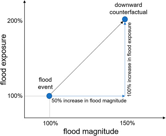
FIGURE 1. Generalized scheme of the proposed method for mapping the sensitivity of floodplains to changes in flood magnitude in terms of exposure using downward counterfactual analysis.

The proposed method extends classical flood risk analyses where the damage-exceedance probability function is used for quantifying flood risk, such as the cost-benefit analysis in flood risk management. The flood exposure or impact is calculated for each flood hazard scenario (return period or exceedance probability, respectively). If plotted on a two-dimensional graph with the exceedance probability of a flood hazard scenario on the x-axis and the number of people exposed as a result of the flood scenario on the y-axis, the exposure footprint of a floodplain can be derived. The slope of the interpolated curve between the basepoints of the hazard scenarios shows how an increase in the probability of a flood relates to an increase in the exposed population, and the range of flood magnitudes over which the sensitivity of the floodplain is highest can be identified. For example, a river reach or floodplain without lateral levees or flood protection might exhibit a population, that is, exposed to floods with a return period as low as 50 years, but the rise in exposure will be relatively linear (Figure 2A) with flood magnitude. In contrast, a river with a high standard of flood protection, e.g., with lateral dikes protecting the floodplain from floods with return periods up to 100 years will not be sensitive to an increase in the frequency of floods of lower magnitudes. In contrast, a significant increase in the affected population will occur when the flood magnitude of the river system exceeds the standard of protection (Figure 2B). These floodplains are sensitive to changes in flooding over the middle range of magnitudes. The third example shows a restored river with a large riverbed (Figure 2C). In this, example, an increase in the flood magnitude will only lead to a slight increase in the area inundated, and a steep increase in flood exposure will only occur in the case of an extreme flood. This means that this floodplain is only sensitive to flood magnitudes in the upper extremes. These characteristics of the exposure functions can be simplified by stating whether a curve is convex, concave, or linear. A concave curve (e.g., Figure 2B) indicates that the sensitivity of the exposure of a floodplain to changes in flood magnitude is higher in the lower range, while a convex curve (e.g., Figure 2C) indicates a higher sensitivity in the upper range of magnitudes. A floodplain with a nearly linear form (e.g., Figure 2A) of the exposure footprint function shows the same sensitivity across all flood magnitudes. The curve also allows the identification of the range of flood magnitudes in which the gradient is steepest as well as the magnitude at which abrupt changes in gradient occur.

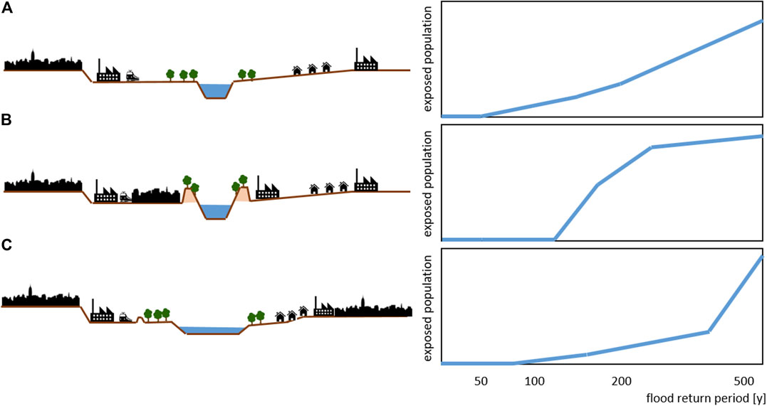
FIGURE 2. Schema of different characteristics of the exposure footprint of the floodplain. (A) A nearly linear increase in the exposed population with increasing flood magnitude. (B) A concave shape, meaning that exposure increases sharply following levee overtopping. This floodplain is sensitive to changes in floods with return periods around the standard of protection. (C) A relatively robust behavior to changes in lower flood magnitudes. This floodplain is mostly sensitive to flood magnitudes in the upper extremes.

In the specific case of climate change, design flood events representative of the current climate can be considered as a starting point for these approaches. The worsening of a today’s design flood event as a result of climatic changes, such as an increase in the frequency or intensity, can be interpreted as a downward counterfactual. The increase in the impact of a current design flood compared to its counterfactual illustrates the sensitivity to changes in hazard. Changes in the frequency or magnitude of specific frequency events are, in fact, the type of indicators that are typically used in the assessment of climate-driven changes in flooding (Arnell and Gosling, 2016). For example, several studies that rely on climate projections have shown that the current 100-years flood can be expected to occur more frequently in many regions over the coming decades, becoming a 10-years return period event in some areas by 2100 (Hirabayashi et al., 2013). It is necessary to understand the sensitivity of our floodplains to these changes and translate this into impacts. Even if climate change predictions are significantly uncertain, which is currently the case, the analysis of sensitivity can offer valuable insights on the types of change that could lead to higher impacts and the adaptation strategies that are best suited to manage the risk. For example, rivers with flood defense structures will not be affected by a substantial increase in the frequency of events below the level of protection but might be affected significantly by a small increase in the magnitude of extreme events.

Prospective Applications

We first tested the application of the proposed method on a local scale using the floodplain of the Emme River between Burgdorf and Gerlafingen in the Canton of Bern, Switzerland, as an example. This example aims to demonstrate the approach based on hydraulic and flood impact simulations only, without the addition of a full model chain of climate/precipitation modeling and hydrologic modeling. The hydraulic simulations were conducted in the 2D BASEMENT modeling environment (Vetsch et al., 2017). The validation of the hydraulic model is described in Zischg et al. (2018d). This numerical model solves the shallow water equations on the basis of an irregular mesh, which was generated from a digital elevation model with a spatial resolution of 0.5 m, as described in detail in Zischg et al. (2018c). In the local case study, flood events were scaled from bankfull discharge (i.e., the river discharge capacity) to very extreme events. The scaling was carried out by increasing the flood magnitude, in a similar manner to that used for sensitivity analysis. To test the different possible indicators, flood magnitude was expressed as a) peak discharge (measured in m³/s), b) extent of the flood (measured in m²), and c) return period (measured in years). Data from the residential register of the Swiss Federal Office of Statistics was used to map the spatial distribution of the residential population, as described in Zischg et al. (2018c). Exposure analysis was then performed at the scale of a single building, and the exposed population was aggregated over the whole floodplain. The floodplain is delimited by the extent of the most extreme flood. When a high number of scenarios is available, as in this case, the gradient can be calculated between pairs of events along the entire range of magnitudes. This allows us to make a detailed analysis of the sensitivity of human exposure on this floodplain to changes over a wide range of flood magnitudes. This example therefore aims to demonstrate changes in the gradient with magnitude.

In the second step, the application of the proposed method was tested at the national scale using Spain as an example. Publicly available flood hazard maps were used together with the associated affected population data compiled by the water basin authorities in Spain. These flood maps, which include the exposed population, represent flood magnitudes with return periods of 10, 100, and 500 years. Both the return period and the extent of flooding are considered indicators of flood magnitude. In the counterfactual analysis for analyzing the sensitivity of floodplains to changes in flood magnitude, the gradient in population exposure between the 1-in-10-years and the 1-in-100-years flood magnitude, and the gradient between the 1-in-100-years and the 1-in-500-years flood magnitude are calculated. The gradients describing the river floodplains and administrative units of the river basin authorities are then mapped. The floodplains are delimited by the topologically connected extent of the most extreme flood. Floodplains that are not connected along the whole of the river are considered floodplains of individual reaches of the river. For visualization purposes, we attribute the calculated gradients to the river lines.

The application of the proposed method was then tested on a global scale using the global flood hazard maps from the European Commission JRC (Alfieri et al., 2016; Dottori et al., 2016; Dottori et al., 2018). The return period was again used as an indicator of flood magnitude and the FLOPROS dataset (Scussolini et al., 2016) was used to consider protection standards. This means that the inundation was set to null for flood maps with return periods below that of the flood protection standard. In contrast to the former example, a population density map from the GPW v4 dataset was used to calculate the number of exposed populations on the basis of population density and the area flooded. The gradients were calculated for the spatially connected floodplains. For visualization purposes, we attribute the calculated gradients to the lines of the main rivers.

Results

The application of this method on a local scale shows the relevance of the indicator used to describe flood magnitude. In this example, 12 synthetic flood events were simulated, ranging from 200 m³/s (return period 1.3 years) to 750 m³/s (return period 960 years), with incremental increases of 50 m³/s in the peak flow (Figures 3 and 4). The 1-in-100 years event has a peak discharge of 600 m³/s. The high number of simulations can be used to assess multiple downward counterfactuals, such as calculating the effect of a downward counterfactual event with an increase of 50 m³/s in peak discharge from several starting points. Downward counterfactual analysis can be performed for flood events of lower as well as for higher magnitudes. In this case, the downward counterfactual analysis corresponds to sensitivity analysis in the conventional sense. The gradient between the flood magnitude and exposed population varies along the axis describing magnitude. When taking the peak discharge as the main indicator for the flood event (i.e., when the magnitude of a flood is perturbed by scaling up the synthetic hydrographs), the floodplains show very linear behavior in terms of changes to flood exposure (Figure 4, left). The number of exposed residents is irrelevant up to a peak discharge of 400 m³/s. This corresponds to a return period of approximately 7.5 years. Above this threshold, the number of residents exposed rises with a steep gradient. The gradient is steeper in the upper range than it is in the lower range of flood magnitudes. In contrast, when return period is used as the indicator for flood magnitude (Figure 4, center), the gradient is steeper in the lower range of magnitudes. This corresponds to the situation in Figure 2B. A curve in between those calculated with the other indicators is obtained when the extent of the flooded area is considered as flood magnitude (Figure 4, right). Here, the gradient is lowest in the middle range of flood magnitudes.

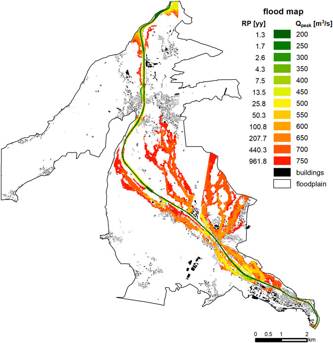
FIGURE 3. Flood map of the Emme River floodplain downstream of Burgdorf, Canton of Bern, Switzerland. The colors show the peak discharge required to flood the spatial subunits and the corresponding return periods.

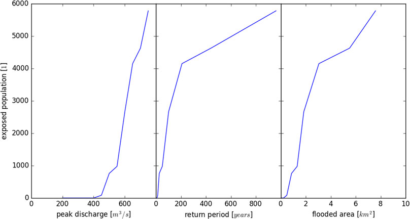
FIGURE 4. Exposure footprint of the Emme River floodplain downstream of Burgdorf, Canton of Bern, Switzerland. Left: Relationship between flood magnitude expressed as peak discharge (m³/s) and exposed population. Center: Relationship between flood magnitude expressed as return period (years) and exposed population. Right: Relationship between flood magnitude expressed as flood extent (km²) and exposed population.

In summary, Figure 4 highlights the importance of the indicator used to describe flood magnitude. Thus, a possible pitfall in applying the proposed method could be a misinterpretation of the absolute values of the sensitivity of a floodplain against changes in flood magnitude. Therefore, the indicator must be explicitly mentioned and care is required when comparing the gradients. As a way of illustration, in the left side of Figure 4, the shape of the curve is mainly determined by the morphology of the river channel, with peak discharges up to 400 m³/s contained within the banks and overflow only occurring at higher discharges. In the right side of Figure 4, the shape of the curve describing exposure is mainly determined by the morphology of the floodplain, producing small changes in inundation up to considerably high discharges. However, these small changes in the area flooded result in significant increases in the exposure values because of the distribution of the population within the floodplain. The population is primarily concentrated along the river, which means that they are affected as soon as the river overflows. The curve in the middle of Figure 4 is determined by the shape of the flood frequency curve, which is nearly a straight line on a semi-logarithmic plot.

This effect of the indicator used to describe flood magnitude is also apparent when the method is applied at a national scale. Figure 5 illustrates the sensitivity of the floodplains of the main rivers in Spain to changes in flood magnitude. In this application, the return period and the flood extent were used as indicators of the flood magnitude and two different flood magnitudes were used for the counterfactual analysis. The first starting point is the event with a return period of 10 years (RP10), and the “perturbed” event is the 1-in-100 years design event (RP100). The gradient is calculated based on the difference between these events (RP10/100). For the higher range of flood magnitudes, the 1-in-100 years design event was selected as the starting point for counterfactual analysis and the 1-in-500 years (RP500) design event as the perturbed event. The gradient is expressed in absolute values, that is, the increase in population exposure (number of people exposed) vs. an increase in the return period (years). It is notable that population exposure shows a high sensitivity to an increasing flood magnitude in some river reaches, while in others the sensitivity differs with the parameter used to indicate magnitude and the range of magnitudes. As shown in the local example, the gradients are, on average, steeper at lower flood magnitudes than at higher magnitudes when return period is considered an indicator of flood magnitude. When flood extent is used as an indicator, the differences between the gradients of the lower and upper magnitude ranges are minor. Interesting examples are the middle reach of the Ebro River in the province of Zaragoza and the rivers at the East coast near Valencia. Flood exposure in these river reaches is sensitive to changes at both magnitude ranges, regardless of the indicator used for the calculation of the gradients. However, only considering the two gradients results in a reduction in the information gathered when compared to that obtained using the entire range of magnitudes, as seen in the application at local scale.

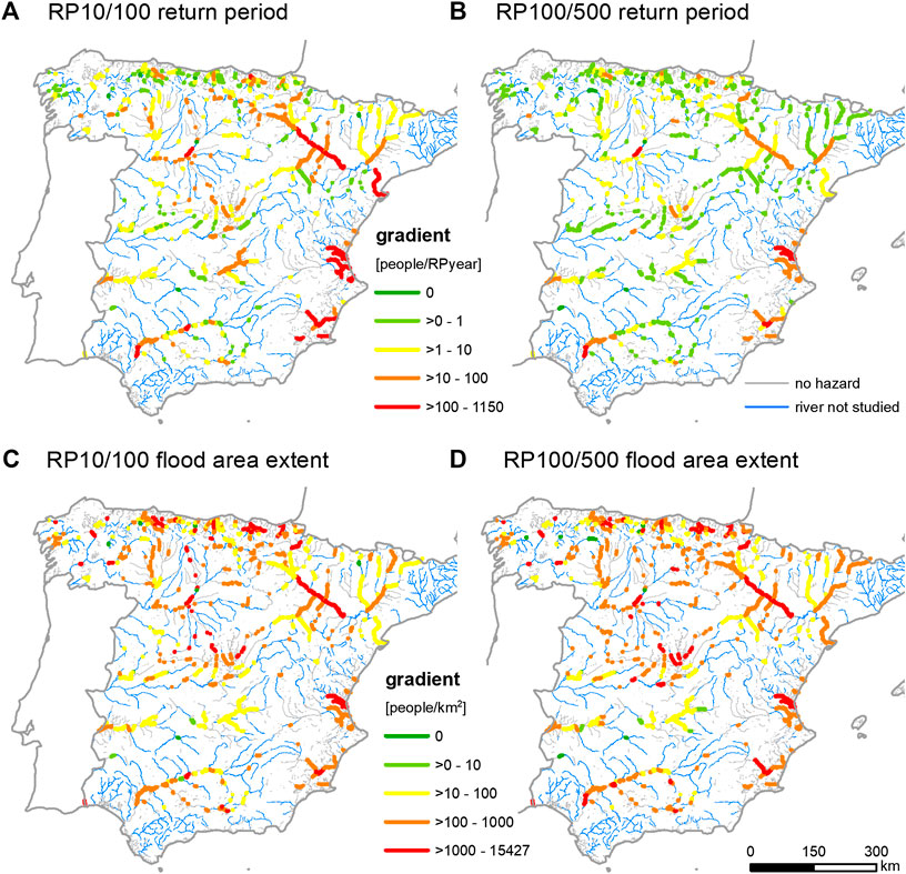
FIGURE 5. Sensitivity of population exposure to changes in flood magnitude in the main river floodplains of Spain: (A) Gradient between an increase in exposed population and an increase in frequency (return period in years) from downward counterfactual analysis of a 1-in-10 years design flood. (B) Gradient derived from downward counterfactual analysis of a 1-in-100 years design flood. (C) Gradient between the increase in the exposed population and the increase in flood extent (km²) from downward counterfactual analysis of a 1-in-10 years design flood. (D) Gradient derived from downward counterfactual analysis of a 1-in-100 years design flood.

Figure 6 shows the normalized gradients of the exposure function, as a complement to the analysis of absolute gradients. The increase in population exposure from the basic scenario to its counterfactual is expressed relative to the population exposure of the basic scenario, as outlined in Figure 1. The increase in the return period is also expressed relative to the return period of the basic scenario. In this way, a gradient of 1 means that a specific percentage increase in the flood magnitude causes an identical percentage increase in the exposure. The spatial pattern of the normalized gradients is similar to that of the absolute gradients when the return period is used as an indicator of flood magnitude. In contrast, the spatial pattern changes when the extent of flooding is used as an indicator of flood magnitude. This is a result of the relatively slight increase in the area flooded caused by an increase in the return period; in many cases this is determined by the orographic lateral constraints of a floodplain. A normalized gradient cannot be calculated if the basic scenario does not affect the population (no exposure), even if the downward counterfactual does. A sudden increase from no exposure to exposure is therefore marked with a different color in Figure 6.

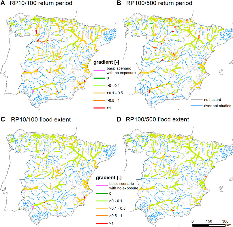
FIGURE 6. Sensitivity of population exposure to changes in the flood magnitude of the main river floodplains of Spain: (A) Normalized gradient between an increase in the exposed population and an increase in the frequency from downward counterfactual analysis of a 1-in-10 years design flood. (B) Normalized gradient derived from downward counterfactual analysis of a 1-in-100 years design flood. (C) Normalized gradient between an increase in the exposed population and an increase in flood extent from the downward counterfactual analysis of a 1-in-10 years design flood. (D) Normalized gradient derived from the downward counterfactual analysis of a 1-in-100 years design flood.

In the application on a global scale, the return periods were used as indicators for flood magnitude and five flood magnitudes were considered for the counterfactual analysis. The first basic scenario is the design event with a return period of 10 years (RP10) and the “perturbed” event is the 1-in-20 years (RP20) event. The gradient was calculated by comparing both events. In the same way, the following pairs of scenarios were considered: RP20/50, RP50/100, RP100/200, and RP200/500. We calculated the normalized gradients, that is, the increase in the exposure and magnitude of the perturbed event relative to the exposure and magnitude of the basic scenario. The gradients vary remarkably across the globe (Figure 7). In the lower range of flood magnitudes, the highest gradients are found in the rivers in South America, Africa, Asia, and Eastern Europe. The Mississippi River system, most European rivers, Indian, and Australian rivers do not show any increase in exposed population when the flood magnitude increases within this range because these rivers have a high flood protection standard. In contrast, the Indian and European rivers show a higher sensitivity in the upper extremes of the flood magnitudes. These flood magnitudes are generally above the standard of protection according to the FLOPROS database. Exceptions are river systems in Western and Eastern United States that have a protection standard for floods of up to a 1-in-200 years design event. Figure 7 indicates that the gradients are overall smaller in the upper range of flood magnitudes than in the lower range. Only 43 river reaches have gradients higher than 1. Figure 8 synthesizes the analyses by highlighting the flood magnitude range with the highest sensitivity gradient. Rivers in South America, Equatorial and Sub Saharan Africa, Eastern Europe, Middle East, and Southeast Asia exhibit the highest sensitivity to changes in flood magnitudes in the lower range (RP10/20, RP20/50). These river reaches have relatively low protection standards and their flood exposure function is concave in shape. In contrast, the rivers of India, North America, Europe, Australia, Asia, and South Africa are more sensitive to changes in the upper range of flood magnitudes (RP100/200, RP200/500) and thus have convex exposure functions. The rivers of Central and East Asia are most sensitive to changes in the upper range of flood magnitudes since they have protection standards in the middle of the flood magnitudes range.

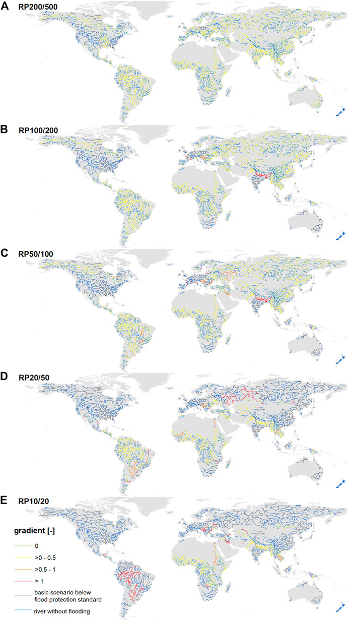
FIGURE 7. Sensitivity of population exposure in the world’s main river floodplains to changes in flood magnitude. Normalized gradient between the increase in exposed population and the increase in frequency from the downward counterfactual analysis of a design flood of (A) 1-in-200 years, (B) 1-in-100 years, (C) 1-in-50 years, (D) 1-in-20 years, and (E) 1-in-10 years.

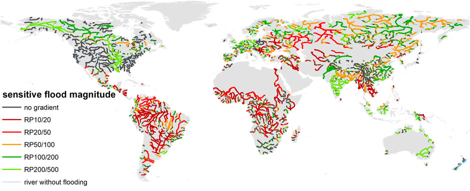
FIGURE 8. Range of flood magnitudes showing the highest relative gradient for sensitivity to change.

Table 1 shows the average gradients for all river reaches where the basic event has a flood exposure greater than 0. If weighted by reach length, the percentage of rivers with no gradients range from 8.8 to 12.7%. The average gradients are generally smaller for the upper flood magnitude ranges. Up to a return period of 100 years, the length-averaged gradients are greater than 1. The maximum gradients range from a factor of 53.2–5,177.8. The maximum gradient can be found in the basic scenario of a return period of 20 years with its counterfactual of 50 years (RP20/50). However, only a small share of rivers has exposure values greater than 0 of floods with return periods up to 20 years.

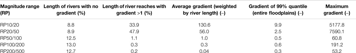
TABLE 1. Mean and maximum values of normalized gradients of river reaches where the basic event has a flood exposure greater than 0.

Discussion

In this study, a method for analyzing and mapping the sensitivity of population exposure in floodplains to changes in the magnitude of flooding was presented. The method is based on downward counterfactuals, namely perturbations of a selected flood scenario by increasing its magnitude. We applied the method at three different scales: local, national, and global. The presented examples demonstrate the significant spatial differences in the exposure of a population to a selected event and its counterfactual. This variability is interesting for further in-depth analysis. The proposed method offers a high potential for gaining insights into why and where settlements and infrastructure in floodplains might be sensitive to climatic changes. This information is mostly contained in flood risk change studies, but the mapping of the gradients allows to make it explicit. The used indicators for flood magnitude are directly correlated. However, the relationship depends on the morphology of the floodplain. The area affected by floods in topographically constrained valleys will not remarkably increase with flood magnitude once the lateral valley slopes are reached. In contrast, the flooded area continuously increases with flood magnitude in flat terrain. The sensitivity indicators can be overlaid with other indicators describing the geomorphological characteristics of floodplains (Allen and Pavelsky, 2018), hydrological characteristics as described in various hydrological datasets, and indicators describing the characteristics of the settlements as well as their topological connectivity to the rivers, as outlined by Zischg et al. (2018a).

The method was proved to be very flexible and applicable on a range of scales. Nevertheless, the suitability of the information content of globally available datasets requires further validation. A thorough comparison between the outcomes of national and global applications must be one of the next steps in the further development of the method. This in turn will enable a robust comparison of the drivers of the sensitivity in different parts of the world.

The calculation of the gradients depends on both the indicator of flood magnitude used and the spatial units in which the gradients are aggregated. In this study, we aggregated the results to topologically connected floodplains, that is, the extent of the maximum flooding of a particular river. If the sensitivity of the floodplain is expressed as the absolute numbers of the increase in exposed population vs. the increase in the area flooded, the numbers will differ between small and large floodplains. Thus, a comparison between spatial units of different sizes is difficult to interpret. The modifiable areal unit problem can be avoided by normalizing gradient values or by harmonizing the spatial units (Röthlisberger et al., 2017); for example, by dividing the river network into reaches of the same length. However, dividing the river networks in this manner also requires dividing the adjacent floodplains into adequate sections for conducting the exposure analysis. The floodplains are preferably delimited on the basis of their geomorphological conditions, and thus we suggest using normalization and calculating relative gradients. Expressing the gradients in relative numbers (i.e., dimensionless) eases interpretation and thus might be preferred for communicating potential risks. A gradient of 1 means that a 1% increase in flood exposure corresponds to a 1% increase in flood magnitude. The normalization enables the comparison of river reaches across wider areas and across a wide range of flood exposures. The maps demonstrating the sensitivity of the floodplains to changes in the flood magnitude can be used to identify river reaches with the highest relative gradients. These river reaches might be the most affected by climate change and thus deserve an in-depth investigation of the underlying characteristics of the floodplains and the potential for climate change adaptation.

On the other hand, the use of absolute numbers to express gradients can support priority setting in national adaptation plans. River reaches with a high increase to exposure in absolute terms might be prioritized over others when developing plans for adapting local or regional flood risk management to the effects of climate change. Analysis at the global scale also showed that the method is sensitive to the standard of flood protection. On a local scale, the standard of flood protection is considered using a high-resolution digital elevation model in the inundation model. The exact river morphology is hardly represented in global scale flood models (Wing et al., 2019). Therefore, the FLOPROS database of flood protection standards was used to consider the effects of measures in river engineering and flood protection. We assumed that no flooding occurs when the return period of the flood map is below the flood protection standard and floods of higher magnitude are not reduced by engineering measures. These assumptions are simplifications and must be considered when interpreting the results. Further analyses must explicitly consider river morphology and flood protection measures. The case studies presented rely on existing data, and the results thus depend significantly on the reliability of the input data.

In the examples shown, we focused only on the exposed population. The method should also be tested in order to analyze application in terms of the sensitivity of infrastructure systems, traffic systems, and other resources that are at risk from changes in flood magnitude. It would be of interest to analyze whether the sensitivity of population exposure differs widely from other types of exposure. However, the application of the presented method for calculating gradients of flood damages will introduce the non-linearity of vulnerability functions in the sensitivity analysis. This effect must be considered when comparing gradients of exposure with gradients of flood damages. Future applications must also focus on the meaning of the gradients and analyze and compare different case studies. However, the explorative application does not allow the assessment of which gradients are to be considered as extreme. The classification of the gradients into legend categories is based on approximative quintiles only.

The exploratory applications showed that the presented exposure-centered approach for mapping the sensitivity of the floodplains to a potential increase in the magnitude of flooding has a high potential for extracting information from flood model applications. This method contributes to understanding the potential drivers of flood risk change; the topological connection between rivers and settlements. The method is neutral to climate scenarios and thus could partially explain the spatial variation in the outcomes of modeling cascades driven by GCMs. This potentially supports the elaboration of narratives and storylines concerning the drivers of future changes in flood risk, and can ultimately contribute to setting priorities for the allocation of financial resources for climate adaptation in flood risk management based on local vulnerabilities (Thaler et al., 2018). Maps of the most sensitive floodplains could support to identify those areas where flood adaptation is needed in a framework of vulnerability-centered flood risk management strategies. However, if cost-benefit analyses and their future changes are needed, climate change simulations are required.

Data Availability Statement

The study was done by using available datasets. These datasets are all cited and listed in the references. Spanish flood maps were downloaded from the website of the “Ministerio para la Transición Ecológica” (MITECO https://www.miteco.gob.es/es/cartografia-y-sig/ide/descargas/agua/zi-lamina.aspx).

Author Contributions

Both authors contributed to the conception and implementation of the study.

Funding

AZ was funded by the Mobiliar Lab for Natural Risks, Oeschger Centre for Climate Change Research, University of Bern. MB was funded by the European Union’s Horizon 2020 research and innovation program under the Marie Skłodowska-Curie Grant Agreement No. 754446 and UGR Research and Knowledge Transfer Fund-Athenea3i. AZ and MB received funds from the University of Granada to support the research stay of AZ at this institution.

Conflict of Interest

The authors declare that the research was conducted in the absence of any commercial or financial relationships that could be construed as a potential conflict of interest.

References

Aerts, J. C. J. H., Botzen, W. J., Clarke, K. C., Cutter, S. L., Hall, J. W., Merz, B., et al. (2018). Integrating human behaviour dynamics into flood disaster risk assessment. Nat. Clim. Change 8, 193–199. doi: 10.1038/s41558-018-0085-1
Alfieri, L., Bisselink, B., Dottori, F., Naumann, G., de Roo, A., Salamon, P., et al. (2016). Global projections of river flood risk in a warmer world. Earth’s Future 5, 171–182. doi: 10.1002/2016EF000485
Allen, G. H., and Pavelsky, T. M. (2018). Global extent of rivers and streams. Science 361, 585–588. doi: 10.1126/science.aat0636
Arnell, N. W., and Gosling, S. N. (2016). The impacts of climate change on river flood risk at the global scale. Clim. Change 134, 387–401. doi: 10.1007/s10584-014-1084-5
Aspinall, W., and Woo, G. (2019). Counterfactual analysis of runaway volcanic explosions. Front. Earth Sci. 7, 1215. doi: 10.3389/feart.2019.00222
Bermúdez, M., and Zischg, A. P. (2018). Sensitivity of flood loss estimates to building representation and flow depth attribution methods in micro-scale flood modelling. Nat. Hazards 92, 1633–1648. doi: 10.1007/s11069-018-3270-7
Broderick, C., Murphy, C., Wilby, R. L., Matthews, T., Prudhomme, C., and Adamson, M. (2019). Using a scenario-neutral framework to avoid potential maladaptation to future flood risk. Water Resour. Res. 16, 1137. doi: 10.1029/2018WR023623
Calka, B., Nowak Da Costa, J., and Bielecka, E. (2017). Fine scale population density data and its application in risk assessment. Geomat. Nat. Hazards Risk 8, 1440–1516. doi: 10.1080/19475705.2017.1345792
CIESIN (2016). High resolution settlement layer (HRSL). Columbia, NY: CIESIN—Facebook Connectivity Lab and Center for International Earth Science Information Network, Columbia University.
Cloke, H. L., Wetterhall, F., He, Y., Freer, J. E., and Pappenberger, F. (2013). Modelling climate impact on floods with ensemble climate projections. Q. J. R. Meteorol. Soc. 139, 282–297. doi: 10.1002/qj.1998
Dottori, F., Salamon, P., Bianchi, A., Alfieri, L., Hirpa, F. A., and Feyen, L. (2016). Development and evaluation of a framework for global flood hazard mapping. Adv. Water Resour. 94, 87–102. doi: 10.1016/j.advwatres.2016.05.002
Dottori, F., Szewczyk, W., Ciscar, J.-C., Zhao, F., Alfieri, L., Hirabayashi, Y., et al. (2018). Increased human and economic losses from river flooding with anthropogenic warming. Nat. Clim. Change 8, 781. doi: 10.1038/s41558-018-0257-z
Felder, G., Gómez-Navarro, J. J., Zischg, A. P., Raible, C. C., Röthlisberger, V., Bozhinova, D., et al. (2018). From global circulation to local flood loss: coupling models across the scales. Sci. Total Environ. 635, 1225–1239. doi: 10.1016/j.scitotenv.2018.04.170
Fleischmann, A., Paiva, R., and Collischonn, W. (2019). Can regional to continental river hydrodynamic models be locally relevant? A cross-scale comparison. J. Hydrol. X 3, 100027. doi: 10.1016/j.hydroa.2019.100027
Fuchs, S., Keiler, M., and Zischg, A. (2015). A spatiotemporal multi-hazard exposure assessment based on property data. Nat. Hazards Earth Syst. Sci. 15, 2127–2142. doi: 10.5194/nhess-15-2127-2015
Fuchs, S., Röthlisberger, V., Thaler, T., Zischg, A., and Keiler, M. (2017). Natural hazard management from a coevolutionary perspective: exposure and policy response in the European Alps. Ann. Assoc. Am. Geogr. 107, 382–392. doi: 10.1080/24694452.2016.1235494
Grimaldi, S., Schumann, G. J.‐P., Shokri, A., Walker, J. P., and Pauwels, V. R. N. (2019). Challenges, opportunities and pitfalls for global coupled hydrologic‐hydraulic modeling of floods. Water Resour. Res. 55, 5277–5300. doi: 10.1029/2018WR024289
Güneralp, B., Güneralp, İ., and Liu, Y. (2015). Changing global patterns of urban exposure to flood and drought hazards. Global Environ. Change 31, 217–225. doi: 10.1016/j.gloenvcha.2015.01.002
Guo, D., Westra, S., and Maier, H. R. (2017). Use of a scenario-neutral approach to identify the key hydro-meteorological attributes that impact runoff from a natural catchment. J. Hydrol. 554, 317–330. doi: 10.1016/j.jhydrol.2017.09.021
Guo, D., Westra, S., and Maier, H. R. (2018). An inverse approach to perturb historical rainfall data for scenario-neutral climate impact studies. J. Hydrol. 556, 877. doi: 10.1016/j.jhydrol.2016.03.025
Gusyev, M., Gädeke, A., Cullmann, J., Magome, J., Sugiura, A., Sawano, H., et al. (2016). Connecting global- and local-scale flood risk assessment: a case study of the Rhine River basin flood hazard. J. Flood Risk Manage. 9, 343–354. doi: 10.1111/jfr3.12243
Hirabayashi, Y., Mahendran, R., Koirala, S., Konoshima, L., Yamazaki, D., Watanabe, S., et al. (2013). Global flood risk under climate change. Nat. Clim. Change 3, 816–821. doi: 10.1038/nclimate1911
IPCC (2012). Managing the risks of extreme events and disasters to advance climate change adaptation: special report of the Intergovernmental Panel on Climate Change. New York, NY: Cambridge University Press, Vol. x, 582.
Jones, B., O’Neill, B. C. (2016). Spatially explicit global population scenarios consistent with the shared socioeconomic pathways. Environ. Res. Lett. 11, 084003. doi: 10.1088/1748-9326/11/8/084003
Jongman, B., Ward, P. J., and Aerts, J. C. J. H. (2012). Global exposure to river and coastal flooding: long term trends and changes. Global Environ. Change 22, 823–835. doi: 10.1016/j.gloenvcha.2012.07.004
Kc, S., and Lutz, W. (2017). The human core of the shared socioeconomic pathways: population scenarios by age, sex and level of education for all countries to 2100. Global Environ. Change 42, 181–192. doi: 10.1016/j.gloenvcha.2014.06.004
Keller, L., Rössler, O., Martius, O., and Weingartner, R. (2019a). Comparison of scenario‐neutral approaches for estimation of climate change impacts on flood characteristics. Hydrol. Process. 33, 535–550. doi: 10.1002/hyp.13341
Keller, L., Zischg, A. P., Mosimann, M., Rössler, O., Weingartner, R., and Martius, O. (2019b). Large ensemble flood loss modelling and uncertainty assessment for future climate conditions for a Swiss pre-alpine catchment. Sci. Total Environ. 693, 133400. doi: 10.1016/j.scitotenv.2019.07.206
Kim, D., Chun, J. A., and Aikins, C. M. (2018). An hourly-scale scenario-neutral flood risk assessment in a mesoscale catchment under climate change. Hydrol. Process. 32, 3416. doi: 10.1002/hyp.13273
Kinoshita, Y., Tanoue, M., Watanabe, S., and Hirabayashi, Y. (2018). Quantifying the effect of autonomous adaptation to global river flood projections: application to future flood risk assessments. Environ. Res. Lett. 13, 014006. doi: 10.1088/1748-9326/aa9401
Knighton, J., Steinschneider, S., and Walter, M. T. (2017). A vulnerability-based, bottom-up assessment of future riverine flood risk using a modified peaks-over-threshold approach and a physically based hydrologic model. Water Resour. Res. 53, 10043–10064. doi: 10.1002/2017WR021036
Kundzewicz, Z. W., Su, B., Wang, Y., Wang, G., Wang, G., and Jiang, T. (2019). Flood risk in a range of spatial perspectives – from global to local scales. Nat. Hazards Earth Syst. Sci. 19, 1319–1328. doi: 10.5194/nhess-19-1319-2019
Lehner, B., Liermann, C. R., Revenga, C., Vörösmarty, C., Fekete, B., Crouzet, P., et al. (2011). High‐resolution mapping of the world’s reservoirs and dams for sustainable river‐flow management. Front. Ecol. Environ. 9, 494–502. doi: 10.1890/100125
Lehner, B., Verdin, K., and Jarvis, A. (2008). New global hydrography derived from spaceborne elevation data. Eos Trans. AGU 89, 93. doi: 10.1029/2008EO100001
Lloyd, C. T., Sorichetta, A., and Tatem, A. J. (2017). High resolution global gridded data for use in population studies. Sci. Data 4, 170001. doi: 10.1038/sdata.2017.1
MARM (2011). Guía metodológica para el desarrollo del sistema. Madrid, Spain: Nacional de Cartografía de Zonas Inundables.
Mateo, C. M. R., Yamazaki, D., Kim, H., Champathong, A., Vaze, J., and Oki, T. (2017). Impacts of spatial resolution and representation of flow connectivity on large-scale simulation of floods. Hydrol. Earth Syst. Sci. 21, 5143–5163. doi: 10.5194/hess-21-5143-2017
Nardi, F., Annis, A., Di Baldassarre, G., Vivoni, E. R., and Grimaldi, S. (2019). GFPLAIN250m, a global high-resolution dataset of Earth’s floodplains. Sci. Data 6, 180309. doi: 10.1038/sdata.2018.309
Pappenberger, F., Dutra, E., Wetterhall, F., and Cloke, H. L. (2012). Deriving global flood hazard maps of fluvial floods through a physical model cascade. Hydrol. Earth Syst. Sci. 16, 4143–4156. doi: 10.5194/hess-16-4143-2012
Prudhomme, C., Reynard, N., and Crooks, S. (2002). Downscaling of global climate models for flood frequency analysis: where are we now? Hydrol. Process. 16, 1137–1150. doi: 10.1002/hyp.1054
Prudhomme, C., Wilby, R. L., Crooks, S., Kay, A. L., and Reynard, N. S. (2010). Scenario-neutral approach to climate change impact studies: application to flood risk. J. Hydrol. 390, 198–209. doi: 10.1016/j.jhydrol.2010.06.043
Roese, N. J. (1997). Counterfactual thinking. Psychol. Bull. 121, 133–148. doi: 10.1037/0033-2909.121.1.133
Roese, N. J., and Olson, J. M. (1995). What might have been: the social psychology of counterfactual thinking. Mahwah, NJ: Lawrence Erlbaum Ass, Vol. XI, 408.
Röthlisberger, V., Zischg, A. P., and Keiler, M. (2017). Identifying spatial clusters of flood exposure to support decision making in risk management, Sci. Total Environ. 598, 593–603. doi: 10.1016/j.scitotenv.2017.03.216
Rozell, D. (2017). Using population projections in climate change analysis. Clim. Change 142, 521–529. doi: 10.1007/s10584-017-1968-2
Sampson, C. C., Smith, A. M., Bates, P. D., Neal, J. C., Alfieri, L., and Freer, J. E. (2015). A high-resolution global flood hazard model. Water Resour. Res. 51, 7358–7381. doi: 10.1002/2015WR016954
Scussolini, P., Aerts, J. C. J. H., Jongman, B., Bouwer, L. M., Winsemius, H. C., de Moel, H., et al. (2016). FLOPROS: an evolving global database of flood protection standards. Nat. Hazards Earth Syst. Sci. 16, 1049–1061. doi: 10.5194/nhess-16-1049-2016
Smith, A., Bates, P. D., Wing, O., Sampson, C., Quinn, N., and Neal, J. (2019). New estimates of flood exposure in developing countries using high-resolution population data. Nat. Commun. 10, 1814. doi: 10.1038/s41467-019-09282-y
Smith, A., Freer, J., Bates, P., and Sampson, C. (2014). Comparing ensemble projections of flooding against flood estimation by continuous simulation. J. Hydrol. 511, 205–219. doi: 10.1016/j.jhydrol.2014.01.045
Staffler, H., Pollinger, R., Zischg, A., and Mani, P. (2008). Spatial variability and potential impacts of climate change on flood and debris flow hazard zone mapping and implications for risk management. Nat. Hazards Earth Syst. Sci. 8, 539–558. doi: 10.5194/nhess-8-539-2008
Steinschneider, S., McCrary, R., Mearns, L. O., and Brown, C. (2015a). The effects of climate model similarity on probabilistic climate projections and the implications for local, risk-based adaptation planning. Geophys. Res. Lett. 42, 5014–5044. doi: 10.1002/2015GL064529
Steinschneider, S., Wi, S., and Brown, C. (2015b). The integrated effects of climate and hydrologic uncertainty on future flood risk assessments. Hydrol. Process. 29, 2823–2839. doi: 10.1002/hyp.10409
Stevens, F. R., Gaughan, A. E., Linard, C., and Tatem, A. J. (2015). Disaggregating census data for population mapping using random forests with remotely-sensed and ancillary data. PloS One 10, e0107042. doi: 10.1371/journal.pone.0107042
Tatem, A. J. (2017). WorldPop, open data for spatial demography. Sci. Data 4, 170004. doi: 10.1038/sdata.2017.4
Thaler, T., Zischg, A., Keiler, M., and Fuchs, S. (2018). Allocation of risk and benefits-distributional justices in mountain hazard management. Reg. Environ. Change 18, 353–365. doi: 10.1007/s10113-017-1229-y
Tiecke, T. G., Liu, X., Zhang, A., Gros, A., Li, N., Yetman, G., et al. (2017). Mapping the world population one building at a time. World Bank. doi: 10.1596/33700
Trigg, M. A., Birch, C. E., Neal, J. C., Bates, P. D., Smith, A., Sampson, C. C., et al. (2016). The credibility challenge for global fluvial flood risk analysis. Environ. Res. Lett. 11, 094014. doi: 10.1088/1748-9326/11/9/094014
UNISDR (2015). Making development sustainable: the future of disaster risk management, Global assessment report on disaster risk reduction. Geneva, Switzerland: United Nations, 311.
Vetsch, D., Siviglia, A., Ehrbar, D., Facchini, M., Gerber, M., Kammerer, S., et al. (2017). BASEMENT—basic simulation environment for Computation of environmental flow and natural hazard simulation. Zurich, Switzerland: ETH Zürich.
Ward, P. J., Jongman, B., Salamon, P., Simpson, A., Bates, P., De Groeve, T., et al. (2015). Usefulness and limitations of global flood risk models. Nat. Clim. Change 5, 712–715. doi: 10.1038/nclimate2742
Ward, P. J., Jongman, B., Weiland, F. S., Bouwman, A., van Beek, R., Bierkens, M. F. P., et al. (2013). Assessing flood risk at the global scale: model setup, results, and sensitivity. Environ. Res. Lett. 8, 044019. doi: 10.1088/1748-9326/8/4/044019
Wing, O. E. J., Bates, P. D., Neal, J. C., Sampson, C. C., Smith, A. M., Quinn, N., et al. (2019). A new automated method for improved flood defense representation in large‐scale hydraulic models. Water Resour. Res. 55, 11007–11034. doi: 10.1029/2019WR025957
Winsemius, H. C., Aerts, J. C. J. H., van Beek, L. P. H., Bierkens, M. F. P., Bouwman, A., Jongman, B., et al. (2015). Global drivers of future river flood risk. Nat. Clim. Change 6, 381. doi: 10.1038/nclimate2893
Winsemius, H. C., Jongman, B., Veldkamp, T. I. E., Hallegatte, S., Bangalore, M., and Ward, P. J. (2018). Disaster risk, climate change, and poverty: assessing the global exposure of poor people to floods and droughts. Environ. Dev. Econ. 56, 1–21. doi: 10.1017/S1355770X17000444
Winsemius, H. C., Van Beek, L. P. H., Jongman, B., Ward, P. J., and Bouwman, A. (2013). A framework for global river flood risk assessments. Hydrol. Earth Syst. Sci. 17, 1871–1892. doi: 10.5194/hess-17-1871-2013
Woo, G. (2019). Downward counterfactual search for extreme events. Front. Earth Sci. 7, 7. doi: 10.3389/feart.2019.00340
Yamazaki, D., Ikeshima, D., Sosa, J., Bates, P. D., Allen, G., and Pavelsky, T. (2019). MERIT hydro: a high‐resolution global hydrography map based on latest topography datasets. Water Resour. Res. 55, 5053–5073. doi: 10.1029/2019WR024873
Zischg, A. P., Felder, G., Mosimann, M., Röthlisberger, V., and Weingartner, R. (2018a). Extending coupled hydrological-hydraulic model chains with a surrogate model for the estimation of flood losses. Environ. Model. Softw. 108, 174–185. doi: 10.1016/j.envsoft.2018.08.009
Zischg, A. P., Felder, G., Weingartner, R., Quinn, N., Coxon, G., Neal, J., et al. (2018b). Effects of variability in probable maximum precipitation patterns on flood losses. Hydrol. Earth Syst. Sci. 22, 2759–2773. doi: 10.5194/hess-22-2759-2018
Zischg, A. P., Hofer, P., Mosimann, M., Röthlisberger, V., Ramirez, J. A., Keiler, M., et al. (2018c). Flood risk (d)evolution: disentangling key drivers of flood risk change with a retro-model experiment. Sci. Total Environ. 639, 195–207. doi: 10.1016/j.scitotenv.2018.05.056
Zischg, A. P., Mosimann, M., Bernet, D. B., and Röthlisberger, V. (2018d). Validation of 2D flood models with insurance claims. J. Hydrol. 557, 350–361. doi: 10.1016/j.jhydrol.2017.12.042
Keywords: floodplain, population exposure, climate change sensitivity, flood magnitude, flood risk, local to global scale, downward counterfactual, sensitivity analysis
Citation: Zischg AP and Bermúdez M (2020) Mapping the Sensitivity of Population Exposure to Changes in Flood Magnitude: Prospective Application From Local to Global Scale. Front. Earth Sci. 8:390. doi: 10.3389/feart.2020.534735
Received: 13 February 2020; Accepted: 17 August 2020;
Published: 03 September 2020.
Edited by:
Jorge Eduardo Teixeira Leandro, Technical University of Munich, GermanyReviewed by:
Daniel Caviedes-Voullieme, Brandenburg University of Technology Cottbus-Senftenberg, GermanyDennis Wagenaar, Deltares, Netherlands
Copyright © 2020 Zischg and Bermúdez. This is an open-access article distributed under the terms of the Creative Commons Attribution License (CC BY). The use, distribution or reproduction in other forums is permitted, provided the original author(s) and the copyright owner(s) are credited and that the original publication in this journal is cited, in accordance with accepted academic practice. No use, distribution or reproduction is permitted which does not comply with these terms.
*Correspondence: Andreas Paul Zischg, andreas.zischg@giub.unibe.ch