How to Deal With Multi-Proxy Data for Paleoenvironmental Reconstructions: Applications to a Holocene Lake Sediment Record From the Tian Shan, Central Asia
 Natalie Schroeter1
  Jaime L. Toney2
  Stefan Lauterbach3,4
  Julia Kalanke5
  Anja Schwarz6
  Stefan Schouten7,8
  Gerd Gleixner1*
- 1Max Planck Institute for Biogeochemistry, Research Group Molecular Biogeochemistry, Jena, Germany
- 2School of Geographical and Earth Sciences, University of Glasgow, Glasgow, United Kingdom
- 3Kiel University, Leibniz Laboratory for Radiometric Dating and Stable Isotope Research, Kiel, Germany
- 4Kiel University, Institute of Geosciences, Kiel, Germany
- 5Section 4.3 – Climate Dynamics and Landscape Evolution, GFZ German Research Centre for Geosciences, Potsdam, Germany
- 6Technische Universität Braunschweig, Institute of Geosystems and Bioindication, Braunschweig, Germany
- 7Department of Marine Microbiology and Biogeochemistry, NIOZ Royal Netherlands Institute for Sea Research, Den Burg, Netherlands
- 8Department of Earth Sciences, Faculty of Geosciences, Utrecht University, Utrecht, Netherlands
Multi-proxy investigations on geological archives provide valuable information about environmental variations in the past. As opposed to single-proxy studies, the combination of several proxies can reveal more detailed information and strengthen subsequent paleoenvironmental reconstructions. However, there is still no consensus about how to deal with resulting highly dimensional datasets in a statistical manner. In many cases, the interpretations of multi-proxy datasets rely on visually matching several proxy records, which can lead to incorrect or insufficient interpretations. Here we report an innovative approach that combines the novel dimension reduction technique Uniform Manifold Approximation and Projection (UMAP) and the time series analysis R package asdetect to identify and characterize Holocene environmental phases and phase boundaries in a sediment core from Lake Chatyr Kol, southern Kyrgyzstan. Despite the fact that the Holocene climate evolution of Central Asia has been intensively studied during the last decades, knowledge about regional climate development during the Holocene and the underlying mechanisms is still relatively scarce. We particularly focus on phase transitions and differentiate between event-based shifts as opposed to gradual phase transitions. For this study, long-chain alkenones were used as a paleotemperature proxy and variations in long-chain alkyl diol distributions were ascribed to relative changes of algal input. The compound-specific stable hydrogen isotope compositions (δD) of individual n-alkanes were utilized as paleohydrological proxies, with the δD of mid-chain n-alkanes reflecting changes in the δD of the lake water and the δD of long-chain n-alkanes recording the δD of the meteoric water. We show the potential of modern analysis tools for data-driven paleoenvironmental reconstructions and advocate for their more frequent implementation in multi-proxy studies.
Introduction
Paleoenvironmental reconstructions are essential to elucidate the Earth’s natural environmental variability in the past. This knowledge enables projections for future climate changes by providing possible analogs for future scenarios (Aichner et al., 2015). Proxy analyses provide a unique tool, often quantitative, to gain insights into past climate conditions since instrumental records mostly cover only the last ∼170 years (Guillot et al., 2015). In particular molecular organic geochemical proxies, so-called biomarkers that have been preserved in natural archives have been extensively used in the field of paleoclimatology and paleoenvironment, especially over the last two decades (Eglinton and Eglinton, 2008; Wang et al., 2016). Biomarkers derive from distinct biotic sources and their abundance and composition is diagnostic for environmental parameters of their formation (Meyers, 2003). Although they typically constitute only <5% of bulk organic matter, biomarkers are widely deployed tools for reconstructing past environmental conditions (Aichner et al., 2010; Feng et al., 2015). Combining the analyses of multiple biomarkers has proven to be more robust as opposed to single-proxy analyses because complementary information and thus a broader perspective can be obtained (Birks and Birks, 2006). However, despite the recent methodological advances, the subsequent data-evaluation and interpretation of biomarker analyses are frequently carried out rather subjectively (“by eye”) with little statistical or computational techniques. Consequently, this approach can be misleading and does not exploit the full potential of these complex datasets. Yet, as the number of large datasets increases and the temporal resolution of the data becomes higher, the need for a concordant approach to summarize patterns in complex multi-proxy datasets becomes even greater. Even though techniques for reducing the dimensionality of multi-proxy data already exist and may be suitable for paleoenvironmental datasets, there are still reservations about their applications. Traditionally, the most commonly used method for dimensionality reduction has been Principal Component Analysis (PCA). PCA is a multivariate statistical analysis that utilizes matrix factorization for projecting high-dimensional data on a lower dimensional subspace comprized of the so-called principal components, while retaining the maximum variability present in the original variables (Ringnér, 2008; Abdi and Williams, 2010; Naik, 2018). Thus, by creating new variables, which are linear combinations of the original variables, PCA allows comparing similarities and potential interdependencies between the original variables (Abdi and Williams, 2010). In the context of paleoenvironmental reconstructions, the described function of PCA could be problematic for two reasons: First, as the variance in multi-proxy data spans across scales and PCA primarily seeks major variability components, small-scale variance may be disregarded even though it might still contain important environmental information. And second, paleoenvironmental data are often nonlinear, especially around phase transitions. In many paleoenvironmental studies, the identification of phases and their boundaries is one of the major objectives, yet PCA may be unable to represent the variability at these critical points in time adequately. Therefore, a novel nonlinear dimension reduction technique for visualization has recently been proposed. This technique, Uniform Manifold Approximation and Projection (UMAP), is generally valued for being both locally and globally optimized (McInnes et al., 2018). This means that while it is a neighbor-embedding method that seeks to resolve the local structure within clusters of data points, it can also define the distance between these clusters in a low-dimensional space in such a way that the original global data structure is optimally represented (McInnes et al., 2018). Since its introduction, UMAP has received considerable attention in a variety of fields (Becht et al., 2018; Diaz-Papkovich et al., 2019; Smets et al., 2019), yet has so far not received full attention in paleoenvironmental reconstructions. In a previous study we showed the effectiveness of applying UMAP to biomolecular data obtained from a lake sediment core, allowing to clearly divide the record into distinct phases in a data-driven manner (Schroeter et al., 2020). Nevertheless, it is unclear whether phase boundaries ascertained by UMAP reflect true abrupt shifts in time series, often classified as tipping points (Lenton et al., 2008; Lenton, 2011; Scheffer et al., 2012), or if these changes can also occur gradually within a determined phase. The identification of tipping points is of particular interest since they can shift a system from one state to another, but the objective identification of them in a time series remains challenging (Marwan et al., 2018). Recently, Boulton and Lenton (2019) introduced a statistical method, implemented in R, for detecting abrupt shifts in time series, which is called asdetect. As opposed to other methods of anomalous change detection that search for significant changes in mean values, asdetect differs by looking for significant changes of gradients within the series (Boulton and Lenton, 2019). However, as asdetect was originally designed for single-proxy investigations, the authors emphasize the need for novel or extended statistical analyses that can be applied to multi-proxy datasets.
Here we combine the results of PCA, UMAP and asdetect as an innovative statistical approach to define and characterize phase boundaries in a more robust approach than previously applied in paleoenvironmental studies. We utilized a multi-proxy dataset of terrestrial and aquatic biomarkers obtained from a sediment core from Lake Chatyr Kol, Kyrgyzstan, Central Asia, reflecting hydrological, and environmental changes of the lake and its catchment area, respectively. Located in Central Asia, the Tian Shan is one of the largest mountain ranges in the world, playing an important role in determining the hydrological and climatological regime of northern Central Asia. Owing to the lake’s position at the intercept between the extent of the mid-latitude Westerlies, the Siberian Anticyclone and partially also the Asian monsoon system (Aizen et al., 2001; Cheng et al., 2012), the Tian Shan represents a key location to study paleoenvironmental changes at high resolution. Although different types of natural archives, such as speleothems (Cheng et al., 2012; Wolff et al., 2017), tree-rings (Esper et al., 2002), loess sequences (Machalett et al., 2008) and lake sediments (Ricketts et al., 2001; Beer et al., 2007; Lauterbach et al., 2014; Mathis et al., 2014; Schwarz et al., 2017) have been analyzed during the last two decades to understand climatic and environmental fluctuations in Central Asia, knowledge about the regional climate development during the Holocene and the underlying mechanisms is still relatively scarce.
The multi-proxy assessment in this study includes the analysis of long-chain alkenones (LCAs) and the respective alkenone unsaturation index as a temperature proxy (Brassell et al., 1986). By analyzing long-chain alkyl diols (LCDs) as an indicator for the presence of algae (Rampen et al., 2012), we connect the intra-lake bio-productivity to variable environmental conditions. We further investigated n-alkanes and their stable hydrogen isotope composition (δD) to assess the lake water budget as well as to evaluate contributions of aquatic and terrestrial sources of organic matter. By applying PCA, UMAP, and asdetect to this multi-proxy dataset, we evaluate the potential of these data analysis approaches for multi-proxy datasets, particularly regarding their ability to differentiate between event-based phase transitions and more gradual shifts. Based on our results, we emphasize the necessity of utilizing data-driven and statistical methods for paleoenvironmental and paleoclimatological studies.
Study Area
Lake Chatyr Kol is an endorheic lake located at 3545 m above sea level (a.s.l.) in the southern Kyrgyz Tian Shan (40°37′N, 75°18′E) (Figure 1). Extending ∼12 km in width (NW-SE) and ∼23 km in length (SW–NE), it encompasses a surface area of ∼159 km2, thus being the third largest lake in Kyrgyzstan. The maximum water depth is 20 m. To the north and south, the basin (catchment area 1084 km2) is limited by the At Bashy Range (∼4600 m) and the Torugart Range (>4800 m), respectively. The extensive pasture-covered plains surrounding the lake predominantly consist of eroded Quaternary material from the mountain ranges. Besides several small tributaries and rivers, the Kekagyr River is the largest and only permanent inflow. During summer, the water balance is predominantly influenced by glacier surface melting and summer storm precipitation. The current climatic regime in the Kyrgyz Tian Shan is primarily determined by the interaction between the Siberian anticyclonic circulation and the mid-latitude Westerlies (Aizen et al., 1997; Lauterbach et al., 2014), whose moisture likely originates in the North Atlantic, the Mediterranean and Caspian Sea (Aizen et al., 2001, 2006; Cheng et al., 2016). Mean annual precipitation amounts to ∼300 mm year–1 in this region (Koppes et al., 2008). The high mountain ranges surrounding Lake Chatyr Kol largely prevent the transport of moisture, resulting in dry conditions and reduced winter precipitation, especially in January and February (Aizen et al., 1995, 2001). In summer, convection increases and strengthens unstable atmospheric stratification, leading to a summer maximum of precipitation brought by cold and moist westerly air masses (Aizen et al., 1995, 2001; Bershaw and Lechler, 2019). Mean annual air temperatures in this region are variable; ranging from −0.34°C in Naryn (∼103 km northeast of Lake Chatyr Kol, 2045 m a.s.l.) (Ilyasov et al., 2013) to −7.2°C in Ak Say (∼30 km east of Lake Chatyr Kol, 3135 m a.s.l.) (Giese et al., 2007), with highest temperatures occurring in July and August. These cold and arid conditions also favor the preservation of permafrost soils (Shnitnikov et al., 1978) and thermokarst formations are widely distributed in this region (Abuduwaili et al., 2019). Vegetation in the region is sparse and characterized by desert and semi-desert vegetation with dominance of montane grassland and no trees (Taft et al., 2011). Since the lake is not inhabited by fish, a considerable number of the amphipod species Gammarus alius sp. nov., which is mostly confined to continental freshwater/brackish habitats, have colonized aquatic plants up to a depth of 50 cm (Sidorov, 2012).
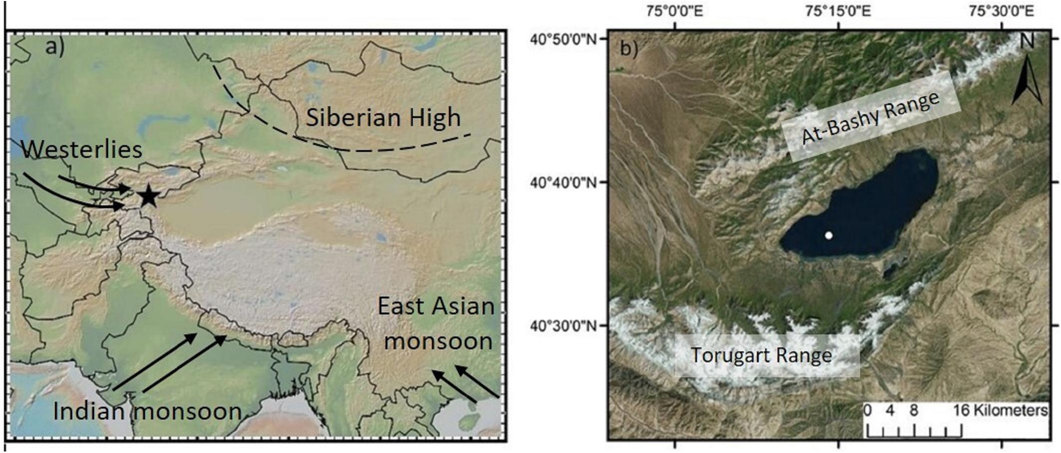
Figure 1. (a) Location of the study site Lake Chatyr Kol (black star) and the dominant circulation systems. (b) Map of Lake Chatyr Kol with coring location (white dot). Figure made with GeoMapApp (www.geomapapp.org).
Materials and Methods
Coring and Chronology
Several vertically overlapping piston cores of 3 m length were retrieved in summer 2012 from a coring site at ∼20 m water depth in the southwestern part of Lake Chatyr Kol (40°36.37′N, 75°14.02′E) by using a 60 mm UWITEC piston corer. In addition, seven gravity cores were collected in autumn 2017 by using a 90 mm UWITEC gravity corer with hammer weight (SC17_1–7). By identification and comparison of distinct macroscopic marker layers, the individual sediment cores could be correlated and merged into a continuous 623.5-cm-long composite profile (Kalanke et al., 2020). By seasonal deposition, the sediments are almost continuously annually laminated (varved) except for the upper 63 cm, allowing the establishment of a floating varve chronology (“Chatvd19”) through microscopic varve counting below 63 cm composite depth (Figure 2). The formation of varves at Lake Chatyr Kol is highly linked to the seasonality of ice coverage during winter and annual variations in temperature and precipitation (Kalanke et al., 2020). A detailed description of the sediments and the age model can be found in Kalanke et al. (2020) and Schroeter et al. (2020). Briefly, microfacies analysis was performed by examining petrographic thin sections, which were prepared at the GFZ German Research Center for Geosciences, Potsdam, Germany, following the method described by Brauer and Casanova (2001). Analysis included counting of individual varves, varve thickness measurements, varve type identification and varve boundary assessment. A total of 11,259 varves were counted twice and interpolated and the mean deviation (∼5%) between the two countings was implemented as the counting uncertainty. Based on the age model, the core has a basal age of 11,619 ± 603 a BP. The floating varve chronology is further supported by accelerator mass spectrometry (AMS) 14C measurements (Poznań Radiocarbon Laboratory, Poznań, Poland) of two wood remains at 380.5 and 528.0 cm composite depth, dating to 6140 ± 137 cal. a BP (Poz-63307) and 9988 ± 203 cal. a BP (Poz-54302), respectively. Calibrated 14C ages (cal. a BP) were calculated in OxCal 4.3 (Bronk Ramsey, 2009) using IntCal13 (Reimer et al., 2013). Gamma spectrometric analysis of 210Pb and 137Cs on continuous 0.5-cm-thick sediment slices of gravity core SC17_7 was performed at the GFZ German Research Center for Geosciences, Potsdam, Germany in order to complement the chronology in the uppermost, non-varved 63 cm of the composite profile (Kalanke et al., 2020). Activity concentrations of 210Pb were incorporated both in a constant initial concentration (CIC) model (Robbins, 1978) and in a constant rate of supply (CRS) model (Appleby and Oldfield, 1978). The onset of enhanced 137Cs concentrations, originating from global nuclear weapon tests (Pennington et al., 1973; Kudo et al., 1998; Wright et al., 1999), was dated to 1945 by both CIC and CRS model assumptions. Consequently, AD 1945 was chosen to constrain the age-depth relationship of the upper homogenous sediments (Kalanke et al., 2020). All ages of Lake Chatyr Kol sediment record mentioned in this study refer to the described age model (Kalanke et al., 2020).
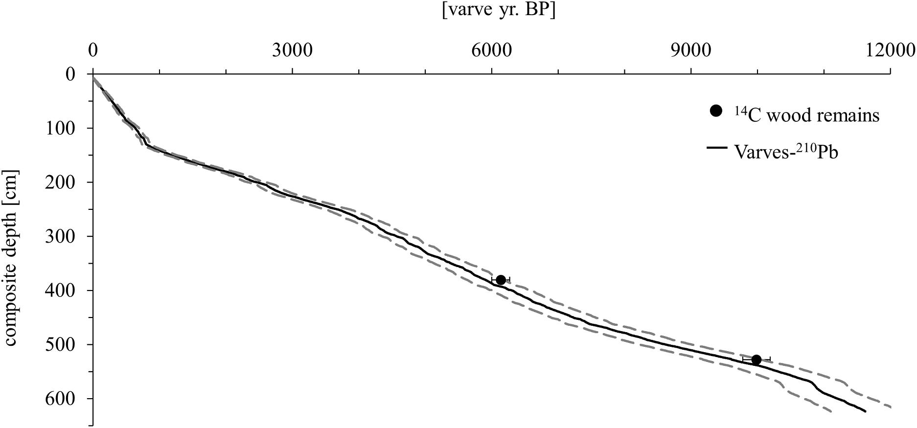
Figure 2. Age model of the Lake Chatyr Kol sediment record. Black dots represent 14C ages of terrestrial macro remains with two σ error ranges. The age model (solid black line) is based on varve counting combined with 210Pb measurements. Dashed lines represent the uncertainty of the varve chronology (Kalanke et al., 2020).
Analysis of Lipid Biomarkers
In total, 89 bulk sediment samples of 1 cm thickness were taken from the composite profile at a mean interval of ∼5 cm. These sediment samples were freeze-dried and extracted in a dichloromethane (DCM) and methanol (MeOH) solvent mixture (9:1, v:v) on a pressurized solvent speed extractor (E-916, BÜCHI, Essen, Germany), which was operated at 100°C and 120 bar for 15 min in two cycles. Biomarker separation was conducted according to Richey and Tierney (2016). The resulting total lipid extract was separated into acid and neutral fractions using aminopropyl gel columns (CHROMABOND® NH2 polypropylene columns, 60 Å, Macherey-Nagel GmbH & Co., KG, Düren, Germany), with neutral compounds eluting in 3:1 DCM:isopropanol and acids eluting in 19:1 diethyl ether:acetic acid. Neutral fractions were further separated over an activated silica gel column (∼2 g, 0.040–0.063 mm mesh, Merck, Darmstadt, Germany) into hydrocarbon (n-alkanes), ketone (alkenones), and polar (diols) fractions by elution with hexane, DCM and MeOH, respectively. Elemental sulfur was removed by adding HCl- activated copper.
Analysis of Sedimentary n-Alkanes
Quantification and identification of n-alkanes were performed on a gas chromatograph with flame ionization detector (GC-FID, Agilent 7890B Gas Chromatograph), based on retention time and peak area comparison with an external n-alkanes standard mixture (nC15 to nC33). Separation of the hydrocarbon fraction was achieved on an Ultra two column (50 m length, 0.32 mm inner diameter, 0.52 μm film thickness, Agilent Technologies, Santa Clara, United States) at a constant helium carrier gas flow of 2 mL min–1. The PTV injector in splitless mode started at 45°C for 0.1 min, then heating up to 300°C with a ramp of 14.5 °C s–1 (held for 3 min). The GC oven temperature program increased from 140°C (held for 1 min) to 310 at 4°C min–1 (held for 15 min) and finally to 325°C with a ramp of 30°C min–1. The final temperature of 325°C was held for 3 min.
The average chain length (ACL) (Poynter and Eglinton, 1990) was calculated according to the following equation:
Analysis of δD of Sedimentary n-Alkanes
δD of the n-alkanes was measured using a coupled GC-IRMS system (GC: HP 7890, Agilent Technologies, Palo Alto United States; IRMS: Delta V Plus, Thermo Fisher Scientific, Bremen, Germany) equipped with a DB1 ms column (length 30 m, 0.25 mm inner diameter, 0.25 μm film thickness; Agilent Technologies, Palo Alto, United States). Column flow was constant at 1.3 ml min–1 and the injector was operated at 280 °C in splitless mode. The oven program started at 110°C (held for 1 min), heated to 320°C (held for 8 min) at a rate of 5°C min–1 and finally to 350°C (held for 3 min) at 30°C min–1. Injection volume was 2 μL and each sample was measured in triplicate followed by a measurement of an external n-alkane standard mixture (nC15 to nC33). The H3+ factor was determined daily to confirm stable ion source conditions and was about 6.8 ± 0.4 over the course of analysis. δD values are reported as per mille relative to VSMOW using the standard δ notation:
where, R = the ratio of deuterium to hydrogen (2H/1H) and VSMOW = Vienna Standard Mean Ocean Water.
The Evaporation-to-Inflow ratio (E/I) was calculated based on the stable isotope approach by Gat and Levy (1978):
with h = relative humidity [0.44 for Lake Chatyr Kol, obtained for the Kashi station 1971–2011 AD, NOAA IGRA (Durre et al., 2006)], δD = stable hydrogen isotope values of lake water (δDnC23) and inflow water (δDnC29) and δD° = limiting isotopic enrichment for a desiccating water body. An average Lake Surface Temperature of 9°C was selected for the calculations. A more detailed explanation of the calculation is provided in Günther et al. (2016).
Analysis of Sedimentary Long-Chain Alkenones
Prior to analysis, ketone fractions containing LCAs were saponified in 0.5 M potassium hydroxide in a MeOH/water solution (95:5, v:v) at 60°C for 12 h (Plancq et al., 2018) to remove alkenoates that could interfere with the identification of LCAs. LCAs were recovered by liquid-liquid extraction using 3 × 1 mL hexane and subsequently analyzed using GC-FID. The analysis was performed at the University of Glasgow, United Kingdom, on an Agilent 7890B GC System equipped with an Agilent VF-200 ms capillary column (60 m length, 0.25 mm inner diameter, 0.10 μm film thickness) (Longo et al., 2013) using hydrogen as carrier gas at a column flow rate of 36 cm s–1. The oven temperature was programmed from 50°C (held for 1 min) to 255 °C at 20 °C min–1, then to 300°C at 3°C min–1 and finally to 320°C at 10°C min–1 followed by 10 min hold time. Peak identification was achieved by gas chromatography-mass spectrometry (GC-MS) using an Agilent 7890B GC coupled with a 5977A GC-EI mass spectrometer and comparing peak retention times and mass spectral data with published data (de Leeuw et al., 1980; Marlowe et al., 1984). The GC conditions were the same as for GC-FID analyses. The MS conditions were as follows: ion energy 70 eV; mass range 40–600 m/z. LCA concentrations were assigned using hexatriacontane (nC36 alkane) as an internal standard. The alkenone unsaturation index was calculated as follows:
A potential alternative alkenone unsaturation index is the index, which excludes contributions of the tetra-unsaturated nC37 methyl alkenone and is frequently utilized in marine settings (e.g. Prahl and Wakeham, 1987; Sikes and Volkman, 1993; Müller et al., 1998; Conte et al., 2006). In lacustrine environments, several studies found a significant relationship of the index and lake water temperature but no correlation between the index and lake water temperature (Toney et al., 2010; Nakamura et al., 2014; Zhao et al., 2017). We therefore chose the index over the index in this study.
Analysis of Sedimentary Long-Chain Alkyl Diols
Polar fractions were analyzed for their LCDs concentration at the Royal Netherlands Institute for Sea Research (NIOZ), Texel, Netherlands. Samples were evaporated to dryness under nitrogen and silylated with a mixture of 10 μL N,O-bis(trimethylsilyl)trifluoroacetamide (BSTFA) and 10 μL pyridine at 60°C for 30 min. Squalane was added as an internal standard. Samples were dissolved in 80 μL ethyl acetate and analyzed by GC-MS using an Agilent 7890B GC equipped with a Agilent CP Sil-5 fused silica capillary column (25 m length, 0.32 mm inner diameter, 0.12 μm film thickness), coupled to an Agilent 5977A MSD mass spectrometer. Instrumental conditions were the same as described by de Bar et al. (2019): the temperature program started at 70°C, increased to 130°C at a rate of 20°C min–1, heated to 320°C at 4°C min–1 and was held at 320°C for 25 min. Flow rate was 2 mL min–1. The quadrupole was held at 150°C and the electron impact ionization energy of the MS source was 70 eV. Fractional abundances were obtained using SIM of m/z = 313.3 (C28 1,13-diol, C30 1,15-diol, C34 1,19-diol) and 341.3 (C30 1,13-diol, C32 1,15-diol, C34 1,17-diol, C36 1,19-diol) ions (Versteegh et al., 1997; Rampen et al., 2012).
Analysis of Diatoms
Subsamples for diatom analyses (∼0.1 g) were taken in 1–32 cm intervals, depending on diatom preservation. If the valves were well preserved, a sample was analyzed at least every 8 cm. Diatom sample preparation followed Kalbe and Werner (1974). The diatom concentration was established by adding known quantities of microspheres (Battarbee and Kneen, 1982). If possible, at least 400 valves were counted in each sample at 1000× magnification and differential interference contrast (DIC) using a Leica DM 5000B microscope. Diatom species were identified based on Lange-Bertalot and Moser (1994); Lange-Bertalot (2001), Oliva et al. (2008); Krammer and Lange-Bertalot (2008), Krammer and Lange-Bertalot (2010); Houk et al. (2010), Hofmann et al. (2011), and Genkal (2012).
Data Analysis
Linear Dimension Reduction by PCA
A PCA was generated using the function “prcomp” in R 3.6 (R Core Team, 2019). The settings for “prcomp” were: scale = TRUE, center = TRUE. The function was supplied with concentrations of the lipid biomarkers and winter solar insolation data at 40°N over the course of the Holocene (Berger and Loutre, 1991). Data visualization was performed using the R package factoextra 1.0.6. (Kassambara and Mundt, 2019) with the function “fviz_pca_var” (repel = TRUE). A scree plot showing the cumulative variance explained by each principal component can be found in Supplementary Figure S1.
Nonlinear Dimension Reduction by UMAP
UMAP was performed using a R 3.6 implementation as package umap 0.2.3.1 (Konopka, 2019; R Core Team, 2019). The UMAP algorithm was supplied with the concentrations of n-alkanes, LCAs, LCDs, the E/I data, the index and the ratio of planktonic and periphytic diatoms. If not specified differently, default options were adopted. To compute the UMAP layout, we used a Manhattan distance metric and fixed the starting conditions to random state = 3 for future reproducibility. A density-based spatial clustering was applied on the resulting layout using the function “hdbscan” within the R package dbscan 1.1-5 and a minimum number of six points per cluster (minPts = 6) (Hahsler et al., 2019). Visualizations of the results were created in the R package ggplot2 3.2.1 (Wickham, 2016).
We also compared the results of UMAP with those of the more commonly used dimensionality reduction technique t-Distributed Stochastic Neighbor Embedding (t-SNE) (Supplementary Figure 2). Both dimension reduction techniques captured the same overall variability pattern. However, UMAP performed better on our dataset as it preserved more of the global structure than t-SNE, resulting in a more distinct clustering using the same settings (Figure 6 and Supplementary Figure S2). Consequently, lake phases were separated more clearly in the UMAP embedding. We therefore implemented the results of UMAP in our further discussion.
Abrupt Shift Detection
Time series analysis was performed using the package asdetect 0.1.0 in R 3.6 (Boulton and Lenton, 2019; R Core Team, 2019). Asdetect was installed using GitHub. The package asdetect was run for each biomarker individually using the default time steps and window lengths fixed between 3 (lowwl) and 1/6 (highwl) of the respective time series. Points in the time series that contribute to significant gradients have a value of 1 added or subtracted to a detection time series, which is then divided by the window length l, resulting in a function-specific detection value.
Results and Discussion
Biomarker Results
Sedimentary n-Alkanes
n-alkanes are aliphatic hydrocarbons that are relatively resistant to degradation (Meyers, 2003). Generally, their distribution and the ACL are used to distinguish different origins of organic matter sources. Long-chain n-alkanes (including nC27, nC29, nC31) with a strong odd-over-even predominance are common components of vascular plant epicuticular waxes (Eglinton and Hamilton, 1967). Therefore, an increase in their concentration would entail higher terrestrial organic productivity (Meyers, 2003). In contrast, short-chain n-alkanes (nC15 to nC19) are synthesized by photosynthetic bacteria and algae (Cranwell et al., 1987; Meyers and Ishiwatari, 1993), whereas submerged and floating aquatic plants produce higher amounts of the mid-chain n-alkanes nC21 to nC25 (Ficken et al., 2000). Consequently, these compounds reflect lacustrine productivity levels (Meyers, 2003).
The sediments of Lake Chatyr Kol contained mainly nC17 and nC23 – nC31 n-alkanes with a strong odd-over-even predominance and a changing distribution pattern within the sediment record (Figure 3). This suggests that the source of n-alkanes primarily derived from allochthonous material (e.g., terrestrial plants). Total n-alkane concentrations ranged from 1.1 to 172.4 μg g–1 dry weight (d.w.) (median: 19.7 μg g–1 d.w., Figure 4). The ACL varied between 17.9 and 29.3, with a median of 25.4. A k-means cluster analysis revealed that the Lake Chatyr Kol sediment record consists of three clusters based on the n-alkane distribution (Figure 3). Sediment samples combined in cluster 1 (n = 13) are characterized by a bimodal pattern of nC23/nC25 and nC29/nC31 (ACL = 26.5), thus reflecting a higher contribution from aquatic macrophytes. Cluster 2 is the most abundant cluster (n = 55), containing primarily long-chain n-alkanes nC27 to nC31 (ACL = 27). Consequently, cluster 2 indicates predominantly terrestrial vegetation input. Cluster 3 is characterized by a dominance of the short-chain n-alkane nC17, therefore suggesting higher proportions of microorganism-derived material, likely from cyanobacteria (Lea-Smith et al., 2015).
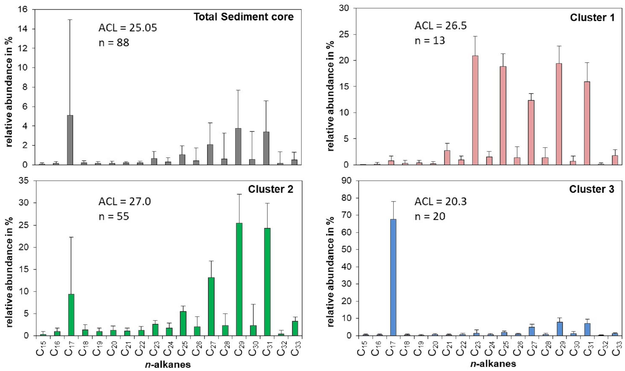
Figure 3. Relative distribution, abundance and ACL [average chain length = Σ(Cn × n)/ΣCn)] of n-alkanes for the entire Lake Chatyr Kol sediment core as well as for the three principal clusters.
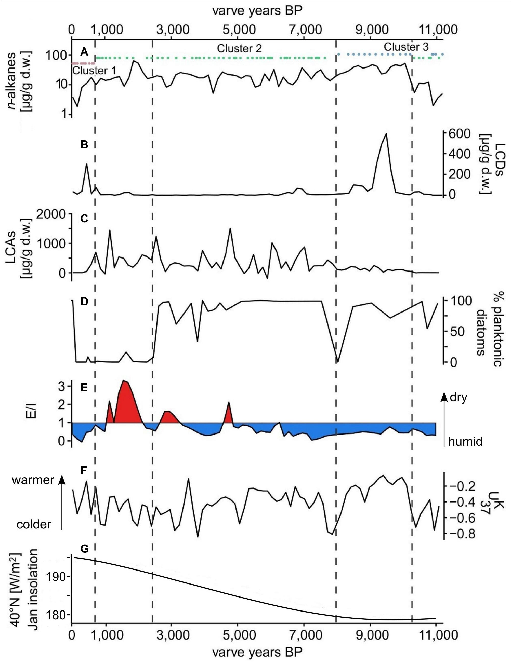
Figure 4. Proxy data from the Lake Chatyr Kol sediment record. (A) total n-alkane amount with n-alkane clusters 1–3; (B) total long-chain alkyl diol amount (LCDs); (C) total long-chain alkenone amount (LCAs); (D) % of planktonic over periphytic diatoms (E) Evaporation-to-inflow ratio (E/I); (F) alkenone unsaturation index ; (G) January insolation at 40°N (Berger and Loutre, 1991). Dashed vertical lines mark phase boundaries defined by UMAP.
δD of Sedimentary n-Alkanes
δD values of n-alkanes are valuable for paleohydrological reconstructions since they mainly record the δD of the source water (Sachse et al., 2012). The δD of the terrestrial n-alkane nC29 thereby reflects the δD signature of the meteoric water (precipitation) modified by evapotranspiration, whereas the δD of the aquatic n-alkane nC23 displays the isotope signal of the ambient lake water, modified by evaporation (Sachse et al., 2012; Guenther et al., 2013). Based on the isotopic differences, the E/I can be applied as a parameter for hydroclimatic balances of a lake system (Mügler et al., 2008). Higher E/I values would indicate higher evaporation relative to input water, therefore reflecting semi-arid or arid environmental conditions. By contrast, humid conditions are characterized by lower E/I values, when inflow water exceeds evaporation (Mügler et al., 2008).
δD of nC23 varied between −56 ‰ at ∼1450 a BP and −165 ‰ at ∼7200 a BP (Supplementary Figure S3). δD of nC29 ranged from −195 ‰ at ∼5900 a BP to −100 ‰ at ∼11,500 a BP, exhibiting smaller fluctuations than the δD of the aquatic nC23 (Supplementary Figure S3). A significant correlation between δDnC23 and δDnC17 throughout the entire sediment record (Pearson correlation coefficient r = 0.48, p < 0.01, Supplementary Figures S3, S4) reinforced the potential of δDnC23 to record changes in the lake water isotopic composition. Reconstructed E/I varied from 0.4 between ∼11,000 and 5000 a BP, pointing to humid conditions, to 0.8 between ∼5000 and 1200 a BP, indicating more arid conditions (Figure 4). The youngest part of the record (∼1000 – 30 a BP) was characterized by an E/I of 0.3, representing more humid conditions (Günther et al., 2016).
Sedimentary Long-Chain Alkenones
LCAs are nC35–nC42 aliphatic unsaturated ketones that are biosynthesized by haptophyte algae from the Isochrysidales order (Theroux et al., 2010). Previous investigations have shown that the occurrence of LCAs in lakes are strongly associated with salinity and stratification (Song et al., 2016; Plancq et al., 2018). Furthermore, the bloom of lacustrine alkenone producers is favored by cold water temperatures and enhanced nutrient availability (Toney et al., 2010). The alkenone unsaturation index , which is based on the correlation of the degree of LCA unsaturation with the temperature of water, is increasingly used to reconstruct surface temperatures in lacustrine settings (Zink et al., 2001; Chu et al., 2005; Toney et al., 2010; Sun et al., 2012). Since LCAs are absent in surface sediments and we cannot exclude multiple haptophyte species inhabiting the lake, which would require DNA analysis, we utilized the index as an indicator for temperature but do not report absolute temperature values.
The concentrations of nC37 and nC38 in the Lake Chatyr Kol sediment record exhibited large variations between 0.3 and 1571 μg g–1 d.w. with a mean of 245 μg g–1 d.w. (Figure 4). Total LCA concentrations included concentrations of the tetra-, tri-, di-unsaturated nC37 methyl alkenones and nC38 ethyl alkenones, as well as tri-unsaturated isomers of nC37 and nC38 alkenones. Values for ranged from −0.873 to −0.057 (median −0.38, Figure 4).
Sedimentary Long-Chain Alkyl Diols
LCDs are a group of lipids that occur widespread in marine environments and consist mainly of saturated C28 and C30 1,13-diols, C28 and C30 1,14-diols, and C30 and C32 1,15-diols (Volkman et al., 1992, 1999; Sinninghe Damsté et al., 2003; Rampen et al., 2014b). These compounds are likely produced by phytoplankton and also appear in freshwater environments (Shimokawara et al., 2010; Castañeda et al., 2011; Romero-Viana et al., 2012; Rampen et al., 2014a; Villanueva et al., 2014; Lattaud et al., 2017, 2018). A major biological source of LCDs in freshwater environments might be the Eustigmatophyceae class of algae, as previous studies have shown a link between the distribution of LCDs and eustigmatophytes (Shimokawara et al., 2010; Rampen et al., 2014a; Villanueva et al., 2014; Lattaud et al., 2018). However, the sources of LCDs as well as environmental controls on the distribution and abundance of LCDs are still poorly known (Rampen et al., 2012, 2014a). In marine settings, sea surface temperatures play an important role in determining abundance and distribution of LCDs (Rampen et al., 2012).
The most abundant LCDs in our sediment core, were the C32 1,15-diol, followed by the C30 1,13-diol. Total LCD content (sum of C28 1,13-diol, C30 1,15-diol, C30 1,13-diol, C32 1,15-diol, C34 1,17-diol, C34 1,19-diol, and C36 1,19-diol) varied between being not detectable and 619 μg g–1 d.w. (Figure 4).
Planktonic and Periphytic Diatoms
Diatoms are frequently utilized as indicators of paleoenvironmental changes (Pérez et al., 2013). Based on the different adaptive strategies, diatoms can be divided into periphytic and planktonic diatoms. Periphytic diatoms colonize and attach to substrates, whereas planktonic diatoms are adapted to floating (Dunck et al., 2013).
In our sediment core, due to temporal changes in valve preservation during the period examined, the diatom concentration strongly varies between 0.0 and 5171.3 × 105 valves g–1 dry weight (Supplementary Figure S5). Zonation of diatom stratification was based on UMAP clustering (see chapter “Lake phases separation”) and additionally visual inspection. Poor diatom preservation up to complete valve dissolution started from about 370 a BP.
Phase I (∼11,000 – 10,200 a BP) and Phase II (∼10,200 – 8050 a BP) are characterized by dominance of planktonic diatoms, mainly Cyclotella choctawhatcheeana Prasad. Periphytic diatoms, e.g., Cocconeis placentula Ehrenberg, are present with varying frequencies. At the beginning of Phase IIIa (∼8050 a BP), periphytic Nitzschia lacuum Lange-Bertalot occurs with higher abundance. Otherwise, the plankton dominance (C. choctawhatcheeana) increases to almost 100% in Phase IIIa. From about 5000 a BP (Phase IIIb) more periphytic diatoms that indicate saline or electrolyte-rich water, such as Achnanthes brevipes var. brevipes Agardh and Navicymbula pusilla (Grunow) Krammer 2003, appear. With the onset of Phase IV (∼2600 – 780 a BP), the diatom assemblages clearly show changes in species composition, planktonic diatoms almost completely disappeared and periphytic species were dominant. From 780 a BP (Phase V) only freshwater periphytic diatoms, mainly C. placentula, occurred in Chatyr Kol. The few valves obtained initially represent periphytic and freshwater-preferring species. In the recent sediments, again planktonic species dominate.
Data Evaluation
Interdependencies Between Biomarkers
The PCA of our biomarker dataset revealed interdependencies between the various biomarker groups and parameters (Figure 5). The winter solar insolation was likely a controlling parameter of the E/I in our sediment record, which in turn affected the concentration of LCAs. Similarly, based on various lake energy and water-balance models, Li and Morrill (2010) found a close relationship between increasing winter solar insolation and increasing lake evaporation throughout the Holocene for monsoonal Asia. Higher E/I values (more arid conditions) would ultimately lead to a higher lake salinity, which likely promoted higher LCA concentrations in our record. Indeed, water salinity has been proposed as one of the determining factors for the occurrence of LCAs in lacustrine environments (Pearson et al., 2008; Toney et al., 2010; Liu et al., 2011; Song et al., 2016). Commonly, LCAs are barely present in both freshwater (0–3 g L–1) and hypersaline (>100 g L–1) lakes, but LCAs are typically found in intermediate salinity freshwater (2.41–44.43 g L–1) settings (Zink et al., 2001; Chu et al., 2005; Liu et al., 2011; Plancq et al., 2018). We therefore deduce a salinity-dependent occurrence of LCAs in Lake Chatyr Kol since LCAs are absent in the lake at the current salinity level of 1.18 g L–1 (measured in July 2018).
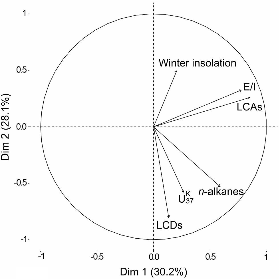
Figure 5. Principal Component Analysis (PCA) visualization of lipid biomarker composition and January insolation at 40°N (Berger and Loutre, 1991) over the Holocene. Accordingly, the winter solar insolation was likely a controlling parameter of the Evaporation-to-Inflow ratio E/I, which in turn affected the presence of LCAs. Conversely, the concentration of both LCDs and n-alkanes seemed to be controlled by temperature ( index).
Conversely, the concentration of both LCDs and n-alkanes seemed to vary with the index (Figure 5). Higher values, suggesting higher temperatures, likely promoted higher occurrences of LCDs as well as n-alkanes. The temperature control on the distribution of LCDs is well observed in marine environments although the sources of the compounds are not clear (Rampen et al., 2012). In contrast, the biological sources of LCDs are likely eustigmatophyte algae (Rampen et al., 2014a; Villanueva et al., 2014). Our results suggest that the productivity of eustigmatophyte algae may have been stimulated by warmer temperatures.
Similar to the occurrence of LCDs, the contribution of n-alkanes seemed to be linked to temperature (Figure 5). Since n-alkanes are dominated by their long-chain homologues in our record, an increase in their concentration would imply an enhanced deposition of allochthonous material. This can be attributed to either higher erosion and/or growth of terrestrial vegetation favored by a warmer climate. Consequently, this could have led to an input of nutrients stimulating eustigmatophyte growth.
Lake Phases Separation
We ran UMAP on the combined dataset of n-alkanes, LCAs, LCDs, E/I, and the ratio of planktonic and periphytic diatoms, containing in total 581 independent data points. A density-based clustering of the resulting UMAP layout separated the sediment core into five distinct phases (I–V), with Phase I: ∼11,000 – 10,200 a BP, Phase II: ∼10,200 – 8050 a BP, Phase III: ∼8050 – 2600 a BP, Phase IV: ∼2600 – 780 a BP, and Phase V: ∼780 – present. Only one data point between Phase I and II remained unclustered (Figure 6).
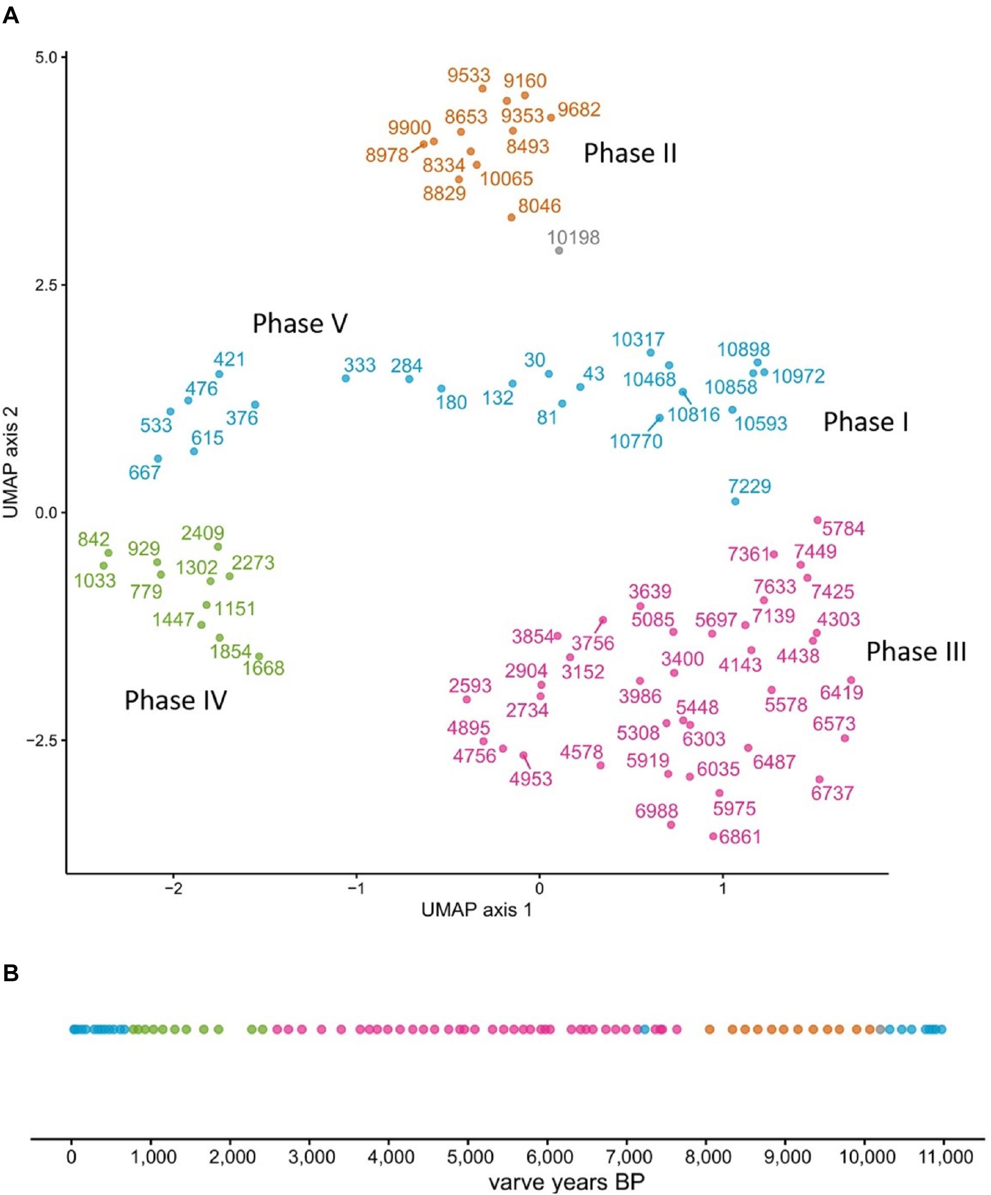
Figure 6. Lake phases separation by UMAP. The core was clustered into 4 separate groupings (A), which when resolved temporally yield five distinct lake phases (B). Note that one data point could not be assigned to a grouping (gray point).
Interestingly, Phase I (∼11,000 – 10,200 a BP) and Phase V (∼780 a BP – present) were assigned to the same cluster (Figure 6), indicating similar environmental conditions. While UMAP clearly identified five temporally separated lake phases, the nature of the transitions between these phases needs further discussion.
Abrupt Shift Detection
To characterize the transitions at the previously identified phase boundaries, we ran asdetect on each proxy separately. Since we had already identified the phase boundaries, we did not apply a threshold to asdetect, but compared the individual results in a combined approach (Figure 7, Supplementary Figure S6). We hypothesized that phase transitions could show two major characteristics. On the one hand a tipping-point type of transition in which an event affects most of biomarker signals simultaneously. On the other hand a gradual phase transition characterized by a consecutive temporal succession of biomarker shifts.
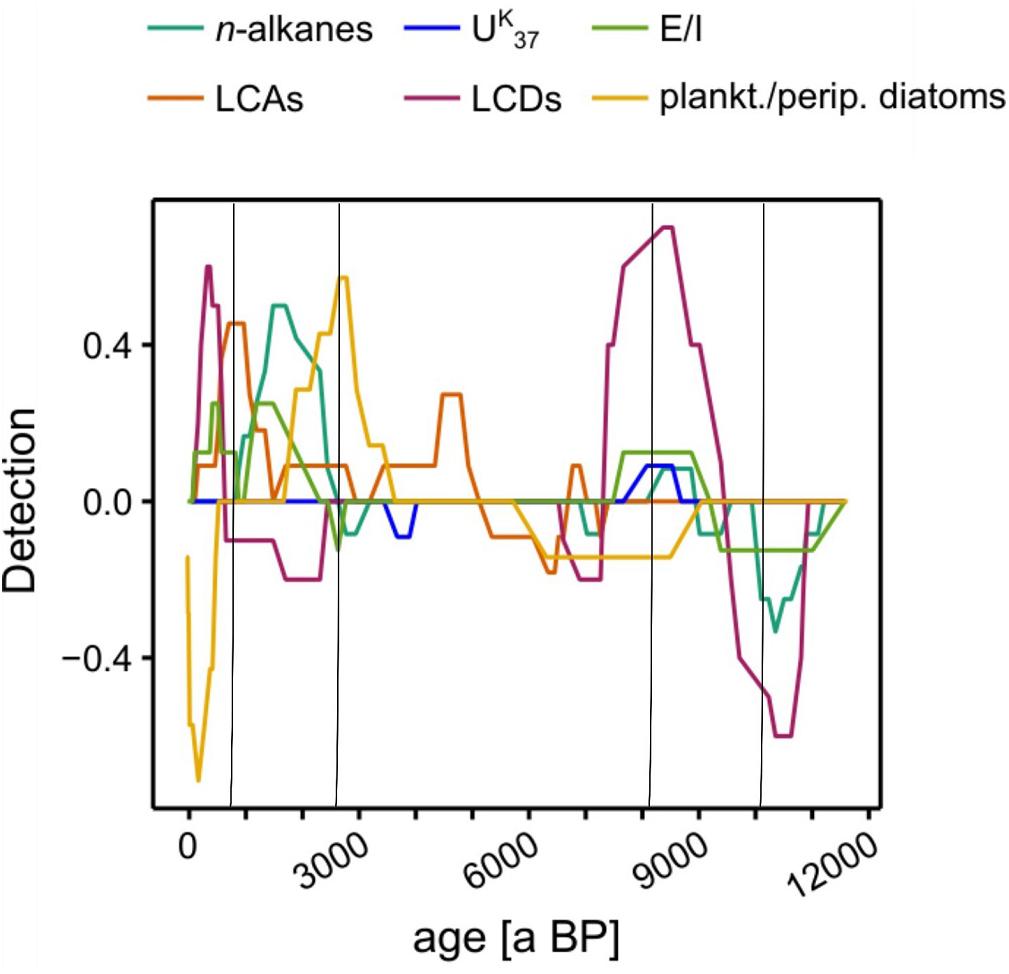
Figure 7. Shift detection results by asdetect. The algorithm was performed on every proxy individually and subsequently stacked. Black lines indicate Phase boundaries defined by UMAP (see Figure 6).
During the Early Holocene, the phase boundaries at ∼10,200 and ∼8050 a BP were characterized by overlapping shift indicators of multiple proxies with their respective maxima/minima at the previously defined phase boundaries (Figure 7). Our data indicate that Early Holocene phase boundaries were likely event-based and could be classified as potential tipping points. In contrast, the phase boundaries in the Late Holocene at ∼2600 and 780 a BP showed less pronounced overlaps of biomarker shifts (Figure 7). Instead, a continuous succession of proxy changes suggests more gradual phase transitions during this period.
Holocene Lake Development
Based on the biomarker results and both lake phases and phase boundary identification, a reconstruction of the lake development over the course of the Holocene was conducted. In accordance with the phase separations, the lake development is discussed in separate sections.
Phase I (∼11,000 – 10,200 a BP)
Phase I comprises the oldest part of the sediment record and is characterized by relatively low concentrations of all biomarkers (Figures 4, 8). Relatively low values and less negative δD values of nC29 (−139 ± 23 ‰) likely reflect cold and arid climate conditions, respectively. Since aquatic plants were most probably not very abundant due to generally low in-lake productivity, concentrations of nC23 are periodically below the limit necessary for reliable δD measurements. Less negative δD values of nC23 at ∼11,000 to 10,900 a BP likely indicate a dry environment.
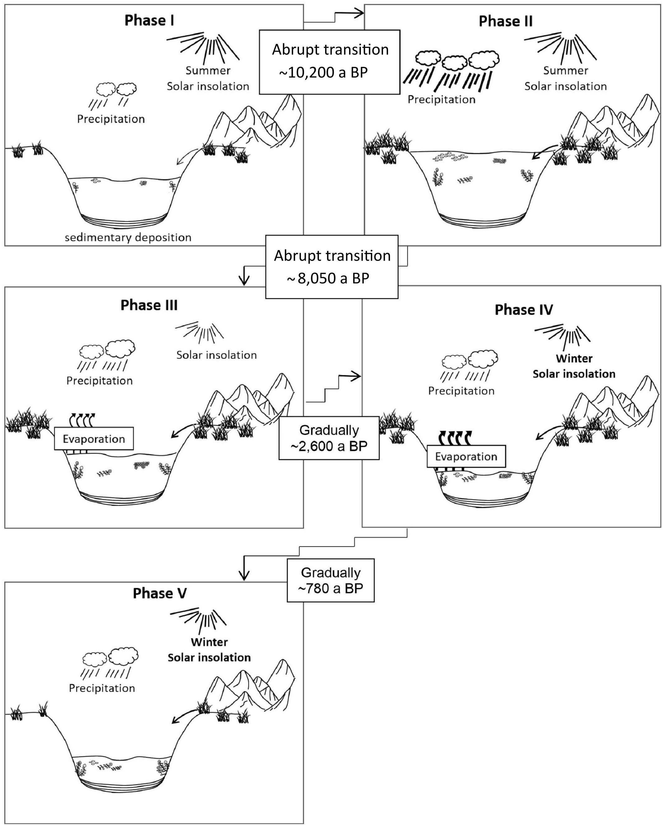
Figure 8. Development of Lake Chatyr Kol during the Holocene. Phases I-V refer to Phase definition by UMAP. Phase boundaries in the Early Holocene (I–II and II–III) were likely event-based while phase boundaries in the Late Holocene (III–IV and IV–V) were likely gradual shifts.
Dominant n-alkane clusters are the terrestrial cluster 2 and the microbial cluster 3 with a dominance of cluster 2 from ∼10,800 to 10,300 a BP. The change at ∼10,900 a BP from cluster 3 to cluster 2 indicates enhanced terrestrial input to the lake system. Concentrations of long-chain n-alkanes were, however, still relatively low. Nevertheless, an increase in the LCD concentration between ∼10,800 and ∼10,300 a BP indicates a slightly increasing biological productivity (Figure 4).
Phase II (∼10,200 – 8050 a BP)
The transition from Phase I to Phase II was likely abrupt. Simultaneous shifts in LCDs, n-alkanes and E/I characterize the transition to Phase II as a potentially event-based tipping point (Figure 7). Rising temperatures as indicated by a sharp increase of , most probably triggered by high summer solar insolation, promoted enhanced terrestrial input and algal productivity as seen in increasing n-alkane and the LCA amounts, respectively. A shift to a dominance of cluster 3, enhanced LCA production and the highest concentrations of LCDs, reflect high productivity of microorganisms due to more favorable lake conditions (Figure 4). The changes in the concentration and distribution of the biomarkers potentially recorded the abrupt crossing of a lake-internal system threshold as a local response to the effects of the Holocene Climate Optimum at ∼10,200 a BP (Figure 4). Low concentrations of nC23 and thus low abundance of aquatic plants most likely reflect a higher lake level and thus a generally deeper lake as in the modern system aquatic plants occur primarily in the shallow water zone (Kalanke et al., 2020). A higher lake level can equally be inferred from the stronger dominance of planktonic over periphytic diatoms in comparison to Phase I (Figures 4, 8). Favorable lake conditions at this time interval were also inferred by Kalanke et al. (2020), who linked the dominating calcite precipitation with enhanced biological activity of e.g., Chrysophyceae and Characeae. Higher temperatures likely led to an isotopic enrichment of the Westerlies-derived precipitation, causing less negative δD values of nC23 (δDnC23 = −132 ± 0.3‰). E/I decreased at ∼10,200 a BP from 0.7 to 0.5, indicating higher moisture availability (Figure 4).
Phase III (∼8050 – 2600 a BP)
A further potential event-based tipping point, identified by simultaneous shifts in LCDs, n-alkanes, E/I and as well as in the planktonic/periphytic diatom ratio marks the onset of Phase III (Figures 7, 8). Warm and relatively stable environmental conditions during Phase II were interrupted by a significant drop of at ∼8050 a BP indicating a shift to colder temperatures (Figure 4). Planktonic diatoms, for instance, were not present at ∼8050 a BP, whereas the dominance of the periphytic diatom Nitzschia lacuum suggests a cooling effect (Supplementary Figure S5). The absence of planktonic diatoms could indicate a strong shortening of the mixing phase, which is the main growth period of planktonic diatoms probably reflected by colder winters (Dreßler et al., 2011). Taking dating uncertainty into account, this cold interval possibly coincides with the North Atlantic 8.2 ka BP event (Alley and Agustsdottir, 2005; Kobashi et al., 2007). Another possibility which would explain the time lag is the hydrogeomorphology of high mountain lakes. The water balance of Lake Chatyr Kol is predominantly regulated by glacier surface melting, which in turn is influenced by air temperatures, solar radiation and precipitation (e.g., Oerlemans, 2005; Pan et al., 2012). However, oftentimes glaciers respond to climate change with a certain time lag (Jóhannesson et al., 1989; Pan et al., 2012), which would ultimately result in a response time lag of the lake. Cold and dry climate conditions during this period were also postulated for the Tibetan Plateau, mostly inferred from pollen data, such as for Lake Qinghai (∼2100 km northeast of Lake Chatyr Kol) at 8.2 cal. ka BP (Shen et al., 2005), Lake Zigetang Co (∼1700 km southeast of Lake Chatyr Kol) at 8700 – 8300 cal. a BP (Herzschuh et al., 2006) and the high mountains of the northeastern Tibetan Plateau (∼2,300 km northeast of Lake Chatyr Kol) at 8300 – 8000 cal. a BP (Miao et al., 2014). Furthermore, the event was observed in stalagmites across China (Dykoski et al., 2005; Wu et al., 2012; Liu et al., 2013). The overlapping timing of the reconstructed dry event ∼8200 years ago in Central Asia, that lasted ∼150 years and the 8.2 ka BP cold event of ∼160 years 8200 years ago observed in Greenland ice cores (Thomas et al., 2007), indicates an atmospheric teleconnection between North Atlantic temperature changes and precipitation in Central Asia. It is suggested that a weakening of the Atlantic Meridional Overturning Circulation affected the North Atlantic, which conversely affected the Asian Monsoon and may be related to changing mean latitudinal position of the Intertropical Convergence Zone (ITCZ) (Hu et al., 2008; Cheng et al., 2009).
A likewise decrease in temperature at Lake Chatyr Kol was also proposed by Kalanke et al. (2020) at ∼8040 a BP based on a shift in the varve microfacies. Phase III also marks the decline of the dominance of microorganisms as seen by a strong decrease in the LCD concentration as well as by a shift to a prevalence of the terrestrial n-alkane cluster 2. Contrary to the decline of microorganisms, concentrations of LCAs increased during Phase III relative to Phase II. Increases in LCA concentrations have been proposed as a stress response to cooler temperatures (Toney et al., 2010).
At ∼6300 – 5800 a BP, δD values of nC29 show the strongest negative values (−191 ± 4‰), possibly associated with high amounts of precipitation and higher lake levels. This would be in agreement with the dating of an exposed lake terrace, which shows a mid-Holocene age of 5786 ± 122 cal. a BP (Kalanke et al., 2020). A dominance of planktonic diatoms (C. choctawhatcheeana) and almost complete disappearance of periphytic diatoms, also indicates higher lake levels around this time. Likewise, more negative δDnC29 values at Lake Son Kol (Central Tian Shan of Kyrgyzstan) suggest predominantly humid summers between 6000 and 4950 cal. a BP (Lauterbach et al., 2014; Schwarz et al., 2017).
Throughout Phase III, however, E/I values increased, indicating increasing dryness likely with a lower lake level. The increase of periphytic diatoms, such as the saline or electrolyte-rich water indicating species A. brevipes var. brevipes and N. pusilla (Hofmann et al., 2011), also suggests lower water levels (Supplementary Figure S5). Lowest values were observed at ∼3900 a BP, which lasted until ∼3600 a BP (Figure 4). Furthermore, Mischke et al. (2010) observed a shift to colder conditions around 3500 cal. a BP for Lake Karakul, NE Tajikistan (∼220 km southwest of Lake Chatyr Kol) by multi-proxy analyses. An alkenone-based study from Lake Balikun, located in the eastern Tian Shan (∼1500 km northeast of Lake Chatyr Kol), showed a similar major cooling between 4800 and 3800 cal. a BP (Zhao et al., 2017). Additionally, a period of dry summers between 4950 and 3900 cal. a BP has been inferred for Lake Son Kol (∼120 km north of Lake Chatyr Kol) (Lauterbach et al., 2014). Cold-arid conditions between 4500 and 3500 cal. a BP have been globally documented and identified as the 4.2 ka BP event (Booth et al., 2005; Staubwasser and Weiss, 2006; Walker et al., 2012). The causes and forcing mechanisms behind the 4.2 ka BP event are still not well understood, but potential explanations include, amongst others, a southward shift of the ITCZ (Mayewski et al., 2004), cooler conditions in the North Atlantic (Bond et al., 1997) and a strengthening of the El Niño Southern Oscillation (Walker et al., 2012; Toth and Aronson, 2019). Recently, Perşoiu et al. (2019) hypothesized that the cold and arid conditions, which prevailed on the Eurasian landmass during the 4.2 ka BP event, resulted from a strengthening and expansion of the Siberian High, which hindered the transport of moisture by blocking the Westerlies. Consequently, this could have caused dry and cold conditions in our study area. Interestingly, both UMAP and asdetect do not characterize this event as a phase boundary nor as an abrupt shift, indicating that the 4.2 ka BP event did not lead to a lake system change in our study area. We therefore hypothesize that an event-based phase transition only occurs after an internal system threshold is exceeded.
Phase IV (∼2600 – 780 a BP)
The transition to Phase IV was initiated by a shift in only a minority of the proxies, which, however, was followed by a consecutive temporal succession of biomarker shifts (Figure 7). At the transition, δDnC23 is more negative, resulting in lower E/I values, pointing to a short-term humid phase (Figure 4). Additionally, the percentage of planktonic diatoms recorded a significant decline. Subsequently, strongly increased E/I values at ∼2300 and ∼1500 a BP characterize arid and warm periods, which led to high evaporation (δDnC23 = −93 ± 21‰) and promoted higher concentrations of LCAs. Over the course of Phase IV, solely periphytic and primarily halophilic diatom species occurred, similarly pointing to lower lake levels and higher salinity, most likely because of higher evaporation (Figure 8). The prevailing warm and dry environmental conditions at ∼2300 and ∼1500 – 1000 a BP coincide with the Roman Warm Period (RWP) and the Medieval Climate Anomaly (MCA), respectively. Similarly, Aichner et al. (2015) found warm and dry episodes at 2500 – 1900 and 1500 – 600 cal. a BP at Lake Karakuli, located at the westernmost edge of Xinjiang Province, China (∼240 km south of Lake Chatyr Kol). Warm conditions during the MCA are also well recorded in tree rings from Western Central Asia, including the Southern Tian Shan (Esper et al., 2002), in pollen data from the Kashgar oasis (∼150 km south of Lake Chatyr Kol) on the western margin of the Tarim Basin (Zhao et al., 2012) and for Lake Bangong Co (∼900 km southeast of Lake Chatyr Kol) (Gasse et al., 1996). During the RWP and the MCA, the lake level was likely lower, which is supported by higher abundances of periphytic diatoms and aquatic plant remains (Kalanke et al., 2020).
Decreased values for both and E/I between ∼1030 and ∼780 a BP imply cold and wet conditions, which is also documented in a number of other paleoclimate records in Central Asia (e.g., Esper et al., 2002; Yang et al., 2009; Chen et al., 2010; Zhao et al., 2012; Aichner et al., 2015) and likely reflects the Little Ice Age (LIA). The predominance of wetter conditions during this interval is in agreement with the presence of exposed paleo-lake deposits that date to 1097 ± 166 cal. a BP and 906 ± 160 cal. a BP (Kalanke et al., 2020).
Phase V (∼780 a BP – Present)
The transition to Phase V was again initiated by a singular proxy shift followed by a lagged response of the remaining proxies (Figure 7). As inferred by UMAP, biomarker profiles during Phase V were comparable to those during Phase I (Figure 6).
The onset of Phase V is reflected by enhanced aquatic productivity, particularly by a shift from the terrestrial n-alkane cluster 2 to the aquatic n-alkane cluster 1 as well as by an increase in LCD concentrations (Figure 4). The shift in the n-alkane composition points to a dominance of submerged macrophytes, whereas, higher amounts of LCDs can be linked to higher values, i.e., increased temperature. In addition, macrophytes dominance is also evidenced by the occurrence of the almost exclusively periphytic C. placentula (Hofmann et al., 2011).
Throughout Phase V, δDnC29 is more negative and an average E/I of 0.3 points toward wetter conditions and higher precipitation in a warmer climate. These conditions likely discriminated against the occurrence of LCAs since their concentration decreased to a minimum (Figure 4). The reconstructed predominantly wet conditions during Phase V are in good agreement with the presence of paleo-lake deposits that date to 530 ± 204 cal. a BP (Kalanke et al., 2020).
At ∼284 a BP the concentrations of LCDs and n-alkanes declined sharply, which could be attributed to decreased values, thus cooler temperatures. Similarly, the concentrations of LCAs remained low, likely induced by a lower E/I, indicating wetter conditions and fresher lake conditions. The inferred predominance of wetter conditions during this interval is in good agreement with the return of planktonic diatoms, which point to rising lake levels (Figures 4, 8).
Conclusion
The present study highlights the applicability of numerical methods for summarizing patterns in complex multi-proxy datasets. By reducing their dimensionality using PCA and UMAP, we increased their interpretability with minimal information loss. PCA allowed for elucidating proxy interdependencies while UMAP and asdetect enabled the objective identification and characterization of lake phases and corresponding phase boundaries, respectively. Over the course of the Holocene, we identified five temporally separated lake phases. In the Early Holocene, phase transitions were likely induced by supra-regional events such as the onset of the Holocene Climate Optimum and the temperature decrease associated with the 8.2 ka BP event. Conversely, during the Late Holocene, phase transitions appeared to have been rather gradual, induced by rather local environmental changes within the catchment area of the lake. Whether event based or gradual, phase transitions at our study site occurred when system-internal thresholds were exceeded as a result of diverse environmental changes.
As one of the rare paleoenvironmental studies integrating data-driven methods, we were able to elucidate the high complexity of lake phase transitions and interdependencies of proxies. We advocate for the use of data-driven approaches to decipher multi-proxy paleoenvironmental records in future studies as an alternative approach to common visual inspection.
Data Availability Statement
The raw data supporting the conclusions of this article will be made available by the authors, without undue reservation.
Author Contributions
GG designed the research idea. SL participated in field work. AS contributed diatom data. JK generated the age chronology. NS carried out laboratory analysis and the data analysis with support from JT and SS. NS prepared the manuscript. All authors discussed the results and improved the manuscript.
Funding
This study was funded by the BMBF-funded research projects CADY (Central Asian Climate Dynamics, Grant No. 03G0813) and CAHOL (Central Asian Holocene Climate, Grant No. 03G0864). NS acknowledges the Max Planck Society and the International Max Planck Research School for Global Biogeochemical Cycles (IMPRS-gBGC) for further project funding.
Conflict of Interest
The authors declare that the research was conducted in the absence of any commercial or financial relationships that could be construed as a potential conflict of interest.
Acknowledgments
We thank Michael Köhler, Sylvia Pinkerneil, Robert Schedel, Denis Henning, Mirlan Daiyrov, and Roman Witt for their involvement in field work. Furthermore we thank Julien Plancq, Steffen Rühlow, Mohammad Ali Salik, and Caglar Yildiz for their assistance during analyses. We also thank Jens Mingram and Achim Brauer for their involvement in the project.
Supplementary Material
The Supplementary Material for this article can be found online at: https://www.frontiersin.org/articles/10.3389/feart.2020.00353/full#supplementary-material
References
Abdi, H., and Williams, L. J. (2010). Principal component analysis. Wiley Interdiscip. Rev. Comput. Stat. 2, 433–459. doi: 10.1002/wics.101
Abuduwaili, J., Issanova, G., and Saparov, G. (2019). Lakes in Kyrgyzstan, Hydrology and Limnology of Central Asia. Singapore: Springer, 288–294. doi: 10.1007/978-981-13-0929-8
Aichner, B., Feakins, S. J., Lee, J. E., Herzschuh, U., and Liu, X. (2015). High-resolution leaf wax carbon and hydrogen isotopic record of the late Holocene paleoclimate in arid Central Asia. Clim. Past 11, 619–633. doi: 10.5194/cp-11-619-2015
Aichner, B., Wilkes, H., Herzschuh, U., Mischke, S., and Zhang, C. (2010). Biomarker and compound-specific δ13C evidence for changing environmental conditions and carbon limitation at Lake Koucha, Eastern Tibetan Plateau. J. Paleolimnol. 43, 873–899. doi: 10.1007/s10933-009-9375-y
Aizen, E. M., Aizen, B., Melack, J. M., Nakamura, T., and Ohta, T. (2001). Precipitation and atmospheric circulation patterns at mid-latitudes of Asia. Int. J. Climatol. 21, 535–556. doi: 10.1002/joc.626
Aizen, V. B., Aizen, E., Joswiak, D. R., Fujita, K., Takeuchi, N., and Nikitin, S. A. (2006). Climatic and atmospheric circulation pattern variability from ice-core isotope/geochemistry records (Altai, Tien Shan and Tibet). Ann. Glaciol. 43, 49–60. doi: 10.3189/172756406781812078
Aizen, V. B., Aizen, E., and Melack, J. (1995). Climate, Snow cover, Glaciers, and Runoff in the Tien Shan, Central Asia. Water Resour. Bull. 31, 1113–1129. doi: 10.1111/j.1752-1688.1995.tb03426.x
Aizen, V. B., Aizen, E., Melack, J., and Dozier, J. (1997). Climatic and hydrologic changes in the Tien Shan, Central Asia. J. Clim. 10, 1393–1404. doi: 10.1175/1520-0442(1997)010<1393:cahcit>2.0.co;2
Alley, R., and Agustsdottir, A. (2005). The 8k event: cause and consequences of a major Holocene abrupt climate change. Quat. Sci. Rev. 24, 1123–1149. doi: 10.1016/j.quascirev.2004.12.004
Appleby, G., and Oldfield, F. (1978). The calculation of lead-210 dates assuming a constant rate of supply of unsupported 210Pb to the sediment. Catena 5, 1–8. doi: 10.1016/S0341-8162(78)80002-2
Battarbee, R. W., and Kneen, M. J. (1982). The use of electronically counted microspheres in absolute diatom analysis. Limnol. Oceanogr. 27, 184–188. doi: 10.4319/lo.1982.27.1.0184
Becht, E., McInnes, L., Healy, J., Dutertre, C. A., Kwok, I. W. H., Ng, L. G., et al. (2018). Dimensionality reduction for visualizing single-cell data using UMAP. Nat. Biotechnol. 37, 38–44. doi: 10.1038/nbt.4314
Beer, R., Heiri, O., and Tinner, W. (2007). Vegetation history, fire history and lake development recorded for 6300 years by pollen, charcoal, loss on ignition and chironomids at a small lake in southern Kyrgyzstan (Alay Range, Central Asia). Holocene 17, 977–985. doi: 10.1177/0959683607082413
Berger, A., and Loutre, M. F. (1991). Insolation values for the climate of the last 10 million years. Quat. Sci. Rev. 10, 297–317. doi: 10.1016/0277-3791(91)90033-Q
Bershaw, J., and Lechler, A. R. (2019). The isotopic composition of meteoric water along altitudinal transects in the Tian Shan of Central Asia. Chem. Geol. 516, 68–78. doi: 10.1016/j.chemgeo.2019.03.032
Birks, H. H., and Birks, H. J. B. (2006). Multi-proxy studies in palaeolimnology. Veg. Hist. Archaeobot. 15, 235–251. doi: 10.1007/s00334-006-0066-6
Bond, G., Showers, W., Cheseby, M., Lotti, R., Almasi, P., DeMenocal, B., et al. (1997). A Pervasive Millennial-Scale Cycle in North Atlantic Holocene and Glacial Climates. Science 278, 1257–1266. doi: 10.1126/science.278.5341.1257
Booth, R. K., Jackson, S. T., Forman, S. L., Kutzbach, J. E., Bettis, E. A., Kreig, J., et al. (2005). A severe centennial-scale drought in mid-continental North America 4200 years ago and apparent global linkages. Holocene 15, 321–328. doi: 10.1191/0959683605hl825ft
Boulton, C. A., and Lenton, T. M. (2019). A new method for detecting abrupt shifts in time series [version 1; peer review: 2 approved with reservations]. F1000 Res. 8:746. doi: 10.12688/f1000research.19310.1
Brassell, S. C., Eglinton, G., Marlowe, I. T., Pflaumann, U., and Sarnthein, M. (1986). Molecular stratigraphy: a new tool for climatic assessment. Nature 320, 129–133. doi: 10.1038/320129a0
Brauer, A., and Casanova, J. (2001). Chronology and depositional processes of the laminated sediment record from Lac d’Annecy, French Alps. J. Paleolimnol. 25, 163–177. doi: 10.1023/A:1008136029735
Bronk Ramsey, C. (2009). Bayesian analysis of radiocarbon dates. Radiocarbon 51, 337–360. doi: 10.1017/s0033822200033865
Castañeda, I. S., Werne, J. P., Johnson, T. C., and Powers, L. A. (2011). Organic geochemical records from Lake Malawi (East Africa) of the last 700years, part II: Biomarker evidence for recent changes in primary productivity. Palaeogeogr. Palaeoclimatol. Palaeoecol. 303, 140–154. doi: 10.1016/j.palaeo.2010.01.006
Chen, F.-H., Chen, J.-H., Holmes, J., Boomer, I., Austin, P., Gates, J. B., et al. (2010). Moisture changes over the last millennium in arid central Asia: a review, synthesis and comparison with monsoon region. Quat. Sci. Rev. 29, 1055–1068. doi: 10.1016/j.quascirev.2010.01.005
Cheng, H., Fleitmann, D., Edwards, R. L., Wang, X., Cruz, F. W., Auler, A. S., et al. (2009). Timing and structure of the 8.2 kyr B.P. event inferred from δ18O records of stalagmites from China, Oman, and Brazil. Geology 37, 1007–1010. doi: 10.1130/G30126A.1
Cheng, H., Spotl, C., Breitenbach, S. F., Sinha, A., Wassenburg, J. A., Jochum, K. P., et al. (2016). Climate variations of Central Asia on orbital to millennial timescales. Sci. Rep. 5:36975. doi: 10.1038/srep36975
Cheng, H., Zhang, Z., Spötl, C., Edwards, R. L., Cai, Y. J., Zhang, D. Z., et al. (2012). The climatic cyclicity in semiarid-arid central Asia over the past 500,000 years. Geophys. Res. Lett. 39:L01705. doi: 10.1029/2011gl050202
Chu, G., Sun, Q., Li, S., Zheng, M., Jia, X., Lu, C., et al. (2005). Long-chain alkenone distributions and temperature dependence in lacustrine surface sediments from China. Geochim. Cosmochim. Acta 69, 4985–5003. doi: 10.1016/j.gca.2005.04.008
Conte, M. H., Sicre, M.-A., Rühlemann, C., Weber, J. C., Schulte, S., Schulz-Bull, D., et al. (2006). Global temperature calibration of the alkenone unsaturation index (UK′37) in surface waters and comparison with surface sediments. Geochem. Geophys. Geosyst. 7:Q02005. doi: 10.1029/2005GC001054
Cranwell, A., Eglinton, G., and Robinson, N. (1987). Lipids of aquatic organisms as potential contributors to lacustrine sediments – II. Org. Geochem. 11, 513–527. doi: 10.1016/0146-6380(87)90007-6
de Bar, M. W., Ullgren, J. E., Thunnell, R. C., Wakeham, S. G., Brummer, G.-J. A., Stuut, J.-B. W., et al. (2019). Long-chain diols in settling particles in tropical oceans: insights into sources, seasonality and proxies. Biogeosciences 16, 1705–1727. doi: 10.5194/bg-16-1705-2019
de Leeuw, J. W., v.d. Meer, F. W., Rijpstra, W. I. C., and Schenck, A. (1980). On the occurrence and structural identification of long chain unsaturated ketones and hydrocarbons in sediments. Phys. Chem. Earth 12, 211–217. doi: 10.1016/0079-1946(79)90105-8
Diaz-Papkovich, A., Anderson-Trocme, L., Ben-Eghan, C., and Gravel, S. (2019). UMAP reveals cryptic population structure and phenotype heterogeneity in large genomic cohorts. PLoS Genet. 15:e1008432. doi: 10.1371/journal.pgen.1008432
Dreßler, M., Schwarz, A., Hübener, T., Adler, S., and Scharf, B. W. (2011). Use of sedimentary diatoms from multiple lakes to distinguish between past changes in trophic state and climate: evidence for climate change in northern Germany during the past 5,000 years. J. Paleolimnol. 45, 223–241.
Dunck, B., Bortolini, J. C., Rodrigues, L., Rodrigues, L. C., Jati, S., and Train, S. (2013). Functional diversity and adaptative strategies of planktonic and periphytic algae in isolated tropical floodplain lake. Braz. J. Bot. 36, 257–266. doi: 10.1007/s40415-013-0029-y
Durre, I., Vose, R. S., and Wuertz, D. B. (2006). Overview of the Integrated Global Radiosonde Archive. J. Clim. 19, 53–68. doi: 10.1175/JCLI3594.1
Dykoski, C., Edwards, R., Cheng, H., Yuan, D., Cai, Y., Zhang, M., et al. (2005). A high-resolution, absolute-dated Holocene and deglacial Asian monsoon record from Dongge Cave, China. Earth Planet. Sci. Lett. 233, 71–86. doi: 10.1016/j.epsl.2005.01.036
Eglinton, G., and Hamilton, R. (1967). Leaf Epicuticular Waxes. Science 156, 1322–1335. doi: 10.1126/science.156.3780.1322
Eglinton, T. I., and Eglinton, G. (2008). Molecular proxies for paleoclimatology. Earth Planet. Sci. Lett. 275, 1–16. doi: 10.1016/j.epsl.2008.07.012
Esper, J., Schweingruber, F. H., and Winiger, M. (2002). 1300 years of climatic history for Western Central Asia inferred from tree-rings. Holocene 12, 267–277. doi: 10.1191/0959683602hl543rp
Feng, X., Gustafsson, Ö, Holmes, R. M., Vonk, J. E., van Dongen, B. E., Semiletov, I. P., et al. (2015). Multimolecular tracers of terrestrial carbon transfer across the pan-Arctic:14C characteristics of sedimentary carbon components and their environmental controls. Glob. Biogeochem. Cycles 29, 1855–1873. doi: 10.1002/2015gb005204
Ficken, K. J., Li, B., Swain, D. L., and Eglinton, G. (2000). An n-alkane proxy for the sedimentary input of submerged/floating freshwater aquatic macrophytes. Org. Geochem. 31, 745–749. doi: 10.1016/S0146-6380(00)00081-4
Gasse, F., Fontes, J. C., Van Campo, E., and Wei, K. (1996). Holocene environmental changes in Bangong Co basin (Western Tibet). Part 4: discussion and conclusions. Palaeogeogr. Palaeoclimatol. Palaeoecol. 120, 79–92. doi: 10.1016/0031-0182(95)00035-6
Gat, J. R., and Levy, Y. (1978). Isotope hydrology of inland sabkhas in Bardawil area. Sinai. Limnol. Oceanogr. 23, 841–850. doi: 10.4319/lo.1978.23.5.0841
Genkal, S. I. (2012). Morphology, taxonomy, ecology, and distribution of Cyclotella choctawhatcheeana prasad (Bacillariophyta). Inland Water Biol. 5, 169–177. doi: 10.1134/S1995082912020046
Giese, E., Mossig, I., Rybski, D., and Bunde, A. (2007). Long-term analysis of air temperature trends in central Asia (Analyse langjähriger Zeitreihen der Lufttemperatur in Zentralasien). Erdkunde 61, 186–202. doi: 10.3112/erdkunde.2007.02.05
Guenther, F., Aichner, B., Siegwolf, R., Xu, B., Yao, T., and Gleixner, G. (2013). A synthesis of hydrogen isotope variability and its hydrological significance at the Qinghai–Tibetan Plateau. Quat. Int. 313-314, 3–16. doi: 10.1016/j.quaint.2013.07.013
Guillot, D., Rajaratnam, B., and Emile-Geay, J. (2015). Statistical paleoclimate reconstructions via Markov random fields. Ann. Appl. Stat. 9, 324–352. doi: 10.1214/14-aoas794
Günther, F., Thiele, A., Biskop, S., Mäusbacher, R., Haberzettl, T., Yao, T., et al. (2016). Late quaternary hydrological changes at Tangra Yumco, Tibetan Plateau: a compound-specific isotope-based quantification of lake level changes. J. Paleolimnol. 55, 369–382. doi: 10.1007/s10933-016-9887-1
Hahsler, M., Piekenbrock, M., and Doran, D. (2019). dbscan: Fast Density-Based Clustering with R. J. Stat. Softw. 91, 1–30. doi: 10.18637/jss.v091.i01
Herzschuh, U., Winter, K., Wünnemann, B., and Li, S. (2006). A general cooling trend on the central Tibetan Plateau throughout the Holocene recorded by the Lake Zigetang pollen spectra. Quat. Int. 154-155, 113–121. doi: 10.1016/j.quaint.2006.02.005
Hofmann, G., Werum, M., and Lange-Bertalot, H. (2011). Diatomeen im Süßwasser - Benthos von Mitteleuropa.: Bestimmungsflora Kieselalgen für die ökologische Praxis. Über 700 der häufigsten Arten und ihre Ökologie. Ruggell: A.R.G. Gantner Verlag.
Houk, V., Klee, R., and Tanaka, H. (2010). Atlas of freshwater centric diatoms with a brief key and descriptions. Part III: Stephanodiscaceae A, Cyclotella, Tertiarius, Discostella. Fottea 10, 1–498.
Hu, C., Henderson, G. M., Huang, J., Xie, S., Sun, Y., and Johnson, K. R. (2008). Quantification of Holocene Asian monsoon rainfall from spatially separated cave records. Earth Planet. Sci. Lett. 266, 221–232. doi: 10.1016/j.epsl.2007.10.015
Ilyasov, S., Zabenko, O., Gaydamak, N., Kirilenko, A., Myrsaliev, N., Shevchenko, V., et al. (2013). Climate Profile of the Kyrgyz Republic, Vol. 99. Bishkek: The United Nations Development Programme.
Jóhannesson, T., Raymond, C., and Waddington, E. (1989). Time–scale for adjustment of glaciers to changes in mass balance. J. Glaciol. 35, 355–369. doi: 10.3189/s002214300000928x
Kalanke, J., Mingram, J., Lauterbach, S., Usubaliev, R., and Brauer, A. (2020). Seasonal deposition processes and chronology of a varved Holocene lake sediment record from Lake Chatyr Kol (Kyrgyz Republic). Geochronology 2, 133–154. doi: 10.5194/gchron-2019-18
Kalbe, L., and Werner, H. (1974). Sediment des Kummerower Sees. Untersuchungen des Chemismus und der Diatomeenflora. Int. Rev. Gesamten Hydrobiol. 59, 755–782. doi: 10.1002/iroh.19740590603
Kassambara, A., and Mundt, F. (2019). factoextra: Extract and Visualize the Results of Multivariate Data Analyses, R package version 1.0.6. Available online at: https://CRAN.R-project.org/package=factoextra (accessed June 1, 2020).
Kobashi, T., Severinghaus, J. P., Brook, E. J., Barnola, J.-M., and Grachev, A. M. (2007). Precise timing and characterization of abrupt climate change 8200 years ago from air trapped in polar ice. Quat. Sci. Rev. 26, 1212–1222. doi: 10.1016/j.quascirev.2007.01.009
Konopka, T. (2019). umap: Uniform Manifold Approximation and Projection. R package version 0.2.3.1. Available online at: https://cran.r-project.org/web/packages/umap/index.html (accessed June 1, 2020).
Koppes, M., Gillespie, A. R., Burke, R. M., Thompson, S. C., and Stone, J. (2008). Late Quaternary glaciation in the Kyrgyz Tien Shan. Quat. Sci. Rev. 27, 846–866. doi: 10.1016/j.quascirev.2008.01.009
Krammer, K., and Lange-Bertalot, H. (2008). Süßwasserflora von Mitteleuropa, 2/2: Bacillariaceae, Epithemiaceae, Surirellaceae. Heidelberg: Spektrum Akademischer Verlag.
Krammer, K., and Lange-Bertalot, H. (2010). Süßwasserflora von Mitteleuropa, 2/1: Naviculaceae. Heidelberg: Spektrum Akademischer Verlag.
Kudo, A., Zheng, J., Koerner, R. M., Fisher, D. A., Santry, D. C., Mahara, Y., et al. (1998). Global transport rates of 137Cs and 239+240Pu originating from the Nagasaki A-bomb in 1945 as determined from analysis of Canadian Arctic ice cores. J. Environ. Radioact. 40, 289–298. doi: 10.1016/S0265-931X(97)00023-4
Lange-Bertalot, H. (2001). “Navicula sensu stricto 10 genera separated from Navicula sensu lato Frustulia,” in Diatoms of Europe, Vol. 2, ed. H. Lange-Bertalot (Ruggell: A.R.H. Gantner Verlag).
Lange-Bertalot, H., and Moser, G. (1994). Brachysira Monographie der Gattung. Bibliotheca Diatomol. 29, 1–212.
Lattaud, J., Dorhout, D., Schulz, H., Castañeda, I. S., Schefuß, E., Sinninghe Damsté, J. S., et al. (2017). The C32 alkane-1,15-diol as a proxy of late Quaternary riverine input in coastal margins. Clim. Past 13, 1049–1061. doi: 10.5194/cp-13-1049-2017
Lattaud, J., Kirkels, F., Peterse, F., Freymond, C. V., Eglinton, T. I., Hefter, J., et al. (2018). Long-chain diols in rivers: distribution and potential biological sources. Biogeosciences 15, 4147–4161. doi: 10.5194/bg-15-4147-2018
Lauterbach, S., Witt, R., Plessen, B., Dulski, P., Prasad, S., Mingram, J., et al. (2014). Climatic imprint of the mid-latitude Westerlies in the Central Tian Shan of Kyrgyzstan and teleconnections to North Atlantic climate variability during the last 6000 years. Holocene 24, 970–984. doi: 10.1177/0959683614534741
Lea-Smith, D. J., Biller, S. J., Davey, M. P., Cotton, C. A. R., Perez Sepulveda, B. M., Turchyn, A. V., et al. (2015). Contribution of cyanobacterial alkane production to the ocean hydrocarbon cycle. Proc. Natl. Acad. Sci. U.S.A. 112, 13591–13596. doi: 10.1073/pnas.1507274112
Lenton, T. M. (2011). Early warning of climate tipping points. Nat. Clim. Change 1, 201–209. doi: 10.1038/nclimate1143
Lenton, T. M., Held, H., Kriegler, E., Hall, J. W., Lucht, W., Rahmstorf, S., et al. (2008). Tipping elements in the Earth’s climate system. Proc. Natl. Acad. Sci. U.S.A. 105, 1786–1793. doi: 10.1073/pnas.0705414105
Li, Y., and Morrill, C. (2010). Multiple factors causing Holocene lake-level change in monsoonal and arid central Asia as identified by model experiments. Clim. Dyn. 35, 1119–1132. doi: 10.1007/s00382-010-0861-8
Liu, W., Liu, Z., Wang, H., He, Y., Wang, Z., and Xu, L. (2011). Salinity control on long-chain alkenone distributions in lake surface waters and sediments of the northern Qinghai-Tibetan Plateau, China. Geochim. Cosmochim. Acta 75, 1693–1703. doi: 10.1016/j.gca.2010.10.029
Liu, Y. H., Henderson, G. M., Hu, C. Y., Mason, A. J., Charnley, N., Johnson, K. R., et al. (2013). Links between the East Asian monsoon and North Atlantic climate during the 8,200 year event. Nat. Geosci. 6, 117–120. doi: 10.1038/ngeo1708
Longo, W. M., Dillon, J. T., Tarozo, R., Salacup, J. M., and Huang, Y. (2013). Unprecedented separation of long chain alkenones from gas chromatography with a poly(trifluoropropylmethylsiloxane) stationary phase. Org. Geochem. 65, 94–102. doi: 10.1016/j.orggeochem.2013.10.011
Machalett, B., Oches, E. A., Frechen, M., Zöller, L., Hambach, U., Mavlyanova, N. G., et al. (2008). Aeolian dust dynamics in central Asia during the Pleistocene: driven by the long-term migration, seasonality, and permanency of the Asiatic polar front. Geochem. Geophys. Geosyst. 9:Q08Q09. doi: 10.1029/2007gc001938
Marlowe, I. T., Brassell, S. C., Eglinton, G., and Green, J. C. (1984). Long chain unsaturated ketones and esters in living algae and marine sediments. Org. Geochem. 6, 135–141. doi: 10.1016/0146-6380(84)90034-2
Marwan, N., Eroglu, D., Ozken, I., Stemler, T., Wyrwoll, K.-H., and Kurths, J. (2018). “Regime change detection in irregularly sampled time series,” in Advances in Nonlinear Geosciences, ed. A. A. Tsonis (Cham: Springer), 357–368. doi: 10.1007/978-3-319-58895-7_18
Mathis, M., Sorrel, P., Klotz, S., Huang, X., and Oberhänsli, H. (2014). Regional vegetation patterns at lake Son Kul reveal Holocene climatic variability in central Tien Shan (Kyrgyzstan, Central Asia). Quat. Sci. Rev. 89, 169–185. doi: 10.1016/j.quascirev.2014.01.023
Mayewski, A., Rohling, E. E., Curt Stager, J., Karlén, W., Maasch, K. A., Meeker, L. D., et al. (2004). Holocene climate variability. Quat. Res. 62, 243–255. doi: 10.1016/j.yqres.2004.07.001
McInnes, L., Healy, J., Saul, N., and Großberger, L. (2018). UMAP: uniform manifold approximation and projection. J. Open Source Softw. 3:861. doi: 10.21105/joss.00861
Meyers, A. (2003). Applications of Organic Geochemistry to paleolimnological reconstructions: a summary of examples from the Laurentian Great Lakes. Org. Geochem. 34, 261–289. doi: 10.1016/s0146-6380(02)00168-7
Meyers, A., and Ishiwatari, R. (1993). Lacustrine Organic Geochemistry.-an overview of indicators of organic matter sources and diagenesis in lake sediments. Org. Geochem. 20, 867–900. doi: 10.1016/0146-6380(93)90100-p
Miao, Y., Jin, H., Liu, B., and Wang, Y. (2014). Natural ecosystem response and recovery after the 8.2 ka cold event: evidence from slope sediments on the northeastern Tibetan Plateau. J. Arid Environ. 104, 17–22. doi: 10.1016/j.jaridenv.2014.01.021
Mischke, S., Rajabov, I., Mustaeva, N., Zhang, C., Herzschuh, U., Boomer, I., et al. (2010). Modern hydrology and late Holocene history of Lake Karakul, eastern Pamirs (Tajikistan): a reconnaissance study. Palaeogeogr. Palaeoclimatol. Palaeoecol. 289, 10–24. doi: 10.1016/j.palaeo.2010.02.004
Mügler, I., Sachse, D., Werner, M., Xu, B., Wu, G., Yao, T., et al. (2008). Effect of lake evaporation on δD values of lacustrine n-alkanes: a comparison of Nam Co (Tibetan Plateau) and Holzmaar (Germany). Org. Geochem. 39, 711–729. doi: 10.1016/j.orggeochem.2008.02.008
Müller, J., Kirst, G., Ruhland, G., von Storch, I., and Rosell-Melé, A. (1998). Calibration of the alkenone paleotemperature index UK’37 based on core-tops from the eastern South Atlantic and the global ocean (60°N-60°S). Geochim. Cosmochim. Acta 62, 1757–1772. doi: 10.1016/S0016-7037(98)00097-0
Nakamura, H., Sawada, K., Araie, H., Suzuki, I., and Shiraiwa, Y. (2014). Long chain alkenes, alkenones and alkenoates produced by the haptophyte alga Chrysotila lamellosa CCMP1307 isolated from a salt marsh. Org. Geochem. 66, 90–97. doi: 10.1016/j.orggeochem.2013.11.007
Oerlemans, J. (2005). Extracting a climate signal from 169 glacier records. Science 308, 675–677. doi: 10.1126/science.1107046
Oliva, M. G., Lugo, A., Alcocer, J., and Cantoral-Uriza, E. (2008). Morphological Study of Cyclotella choctawhatcheeana Prasad (Stephanodiscaceae) from a saline Mexican Lake. Aquat. Biosyst. 4, 17–25. doi: 10.1186/1746-1448-4-17
Pan, B. T., Zhang, G. L., Wang, J., Cao, B., Geng, H. P., Wang, J., et al. (2012). Glacier changes from 1966–2009 in the Gongga Mountains, on the south-eastern margin of the Qinghai-Tibetan Plateau and their climatic forcing. Cryosphere 6, 1087–1101. doi: 10.5194/tc-6-1087-2012
Pearson, E. J., Juggins, S., and Farrimond, P. (2008). Distribution and significance of long-chain alkenones as salinity and temperature indicators in Spanish saline lake sediments. Geochim. Cosmochim. Acta 72, 4035–4046. doi: 10.1016/j.gca.2008.05.052
Pennington, W., Tutin, T. G., Cambray, R. S., and Fisher, E. M. (1973). Observations on Lake Sediments using Fallout 137Cs as a Tracer. Nature 242, 324–326. doi: 10.1038/242324a0
Pérez, L., Lorenschat, J., Massaferro, J., Pailles, C., Sylvestre, F., Hollwedel, W., et al. (2013). Bioindicators of climate and trophic state in lowland and highland aquatic ecosystems of the northern Neotropics. Rev. Biol. Trop. 61, 603–644. doi: 10.15517/rbt.v61i2.11164
Perşoiu, A., Ionita, M., and Weiss, H. (2019). Atmospheric blocking induced by the strengthened Siberian High led to drying in west Asia during the 4.2 ka BP event – a hypothesis. Clim. Past 15, 781–793. doi: 10.5194/cp-15-781-2019
Plancq, J., Cavazzin, B., Juggins, S., Haig, H. A., Leavitt, R., and Toney, J. L. (2018). Assessing environmental controls on the distribution of long-chain alkenones in the Canadian Prairies. Org. Geochem. 117, 43–55. doi: 10.1016/j.orggeochem.2017.12.005
Poynter, J., and Eglinton, G. (1990). Molecular composition of three sediments from Hole 717C: the Bengal fan. Proc. Ocean Drill. Program 116, 155–161. doi: 10.2973/odp.proc.sr.116.151.1990
Prahl, F. G., and Wakeham, S. G. (1987). Calibration of unsaturation patterns in long-chain ketone compositions for palaeotemperature assessment. Nature 330, 367–369. doi: 10.1038/330367a0
R Core Team (2019). R: A Language and Environment for Statistical Computing. Vienna: R Foundation for Statistical Computing.
Rampen, S. W., Datema, M., Rodrigo-Gámiz, M., Schouten, S., Reichart, G.-J., and Sinninghe Damsté, J. S. (2014a). Sources and proxy potential of long chain alkyl diols in lacustrine environments. Geochim. Cosmochim. Acta 144, 59–71. doi: 10.1016/j.gca.2014.08.033
Rampen, S. W., Willmott, V., Kim, J.-H., Rodrigo-Gámiz, M., Uliana, E., Mollenhauer, G., et al. (2014b). Evaluation of long chain 1,14-alkyl diols in marine sediments as indicators for upwelling and temperature. Org. Geochem. 76, 39–47. doi: 10.1016/j.orggeochem.2014.07.012
Rampen, S. W., Willmott, V., Kim, J.-H., Uliana, E., Mollenhauer, G., Schefuß, E., et al. (2012). Long chain 1,13- and 1,15-diols as a potential proxy for palaeotemperature reconstruction. Geochim. Cosmochim. Acta 84, 204–216. doi: 10.1016/j.gca.2012.01.024
Reimer, J., Bard, E., Bayliss, A., Beck, J. W., Blackwell, G., Ramsey, C. B., et al. (2013). IntCal13 and Marine13 Radiocarbon Age Calibration Curves 0–50,000 Years cal BP. Radiocarbon 55, 1869–1887. doi: 10.2458/azu_js_rc.55.16947
Richey, J. N., and Tierney, J. E. (2016). GDGT and alkenone flux in the northern Gulf of Mexico: implications for the TEX86 and UK’37 paleothermometers. Paleoceanography 31, 1547–1561. doi: 10.1002/2016pa003032
Ricketts, R. D., Johnson, T. C., Brown, E. T., Rasmussen, K. A., and Romanovsky, V. (2001). The Holocene paleolimnology of Lake Issyk-Kul, Kyrgyzstan: trace element and stable isotope composition of ostracodes. Palaeogeogr. Palaeoclimatol. Palaeoecol. 176, 207–227. doi: 10.1016/s0031-0182(01)00339-x
Ringnér, M. (2008). What is principal component analysis? Nat. Biotechnol. 26, 303–304. doi: 10.1038/nbt0308-303
Robbins, J. A. (1978). “Geochemical and geophysical applications of radioactive lead,” in Biogeochemistry of Lead in the Environment, ed. J. O. Nriagu (Amsterdam: Elsevier), 285–393.
Romero-Viana, L., Kienel, U., and Sachse, D. (2012). Lipid biomarker signatures in a hypersaline lake on Isabel Island (Eastern Pacific) as a proxy for past rainfall anomaly (1942–2006AD). Palaeogeogr. Palaeoclimatol. Palaeoecol. 350-352, 49–61. doi: 10.1016/j.palaeo.2012.06.011
Sachse, D., Billault, I., Bowen, G. J., Chikaraishi, Y., Dawson, T. E., Feakins, S. J., et al. (2012). Molecular paleohydrology: interpreting the hydrogen-isotopic composition of lipid biomarkers from photosynthesizing organisms. Annu. Rev. Earth Planet. Sci. 40, 221–249. doi: 10.1146/annurev-earth-042711-105535
Scheffer, M., Carpenter, S. R., Lenton, T. M., Bascompte, J., Brock, W., Dakos, V., et al. (2012). Anticipating critical transitions. Science 338, 344–348. doi: 10.1126/science.1225244
Schroeter, N., Lauterbach, S., Stebich, M., Kalanke, J., Mingram, J., Yildiz, C., et al. (2020). Biomolecular evidence of early human occupation of a high-altitude site in Western Central Asia during the Holocene. Front. Earth Sci. 8:20. doi: 10.3389/feart.2020.00020
Schwarz, A., Turner, F., Lauterbach, S., Plessen, B., Krahn, K. J., Glodniok, S., et al. (2017). Mid- to late Holocene climate-driven regime shifts inferred from diatom, ostracod and stable isotope records from Lake Son Kol (Central Tian Shan, Kyrgyzstan). Quat. Sci. Rev. 177, 340–356. doi: 10.1016/j.quascirev.2017.10.009
Shen, J., Liu, X., Wang, S., and Matsumoto, R. (2005). Palaeoclimatic changes in the Qinghai Lake area during the last 18,000 years. Quat. Int. 136, 131–140. doi: 10.1016/j.quaint.2004.11.014
Shimokawara, M., Nishimura, M., Matsuda, T., Akiyama, N., and Kawai, T. (2010). Bound forms, compositional features, major sources and diagenesis of long chain, alkyl mid-chain diols in Lake Baikal sediments over the past 28,000 years. Org. Geochem. 41, 753–766. doi: 10.1016/j.orggeochem.2010.05.013
Shnitnikov, A. V., Livja, A. A., Berdovskaya, G. N., and Sevastianov, D. V. (1978). Paleolimnology of Chatyrkel Lake (Tien-shan). Pol. Arch. Hydrobiol. 25, 38 3–390.
Sidorov, D. A. (2012). Two new species of freshwater amphipods (Crustacea: Gammaridae) from Central Asia, with comments on the unusual upper lip morphology. Zootaxa 3317, 1–24. doi: 10.11646/zootaxa.3317.1.1
Sikes, E., and Volkman, J. K. (1993). Calibration of alkenone unsaturation ratios (UK’37) for paleotemperature estimation in cold polar waters. Geochim. Cosmochim. Acta 57, 1883–1889. doi: 10.1016/0016-7037(93)90120-L
Sinninghe Damsté, J. S., Rampen, S., Irene, W., Rijpstra, C., Abbas, B., Muyzer, G., et al. (2003). A diatomaceous origin for long-chain diols and mid-chain hydroxy methyl alkanoates widely occurring in quaternary marine sediments: indicators for high-nutrient conditions. Geochim. Cosmochim. Acta 67, 1339–1348. doi: 10.1016/s0016-7037(02)01225-5
Smets, T., Verbeeck, N., Claesen, M., Asperger, A., Griffioen, G., Tousseyn, T., et al. (2019). Evaluation of distance metrics and spatial autocorrelation in uniform manifold approximation and projection applied to mass spectrometry imaging data. Anal. Chem. 91, 5706–5714. doi: 10.1021/acs.analchem.8b05827
Song, M., Zhou, A., He, Y., Zhao, C., Wu, J., Zhao, Y., et al. (2016). Environmental controls on long-chain alkenone occurrence and compositional patterns in lacustrine sediments, northwestern China. Org. Geochem. 91, 43–53. doi: 10.1016/j.orggeochem.2015.10.009
Staubwasser, M., and Weiss, H. (2006). Holocene Climate and Cultural Evolution in Late Prehistoric–Early Historic West Asia. Quat. Res. 66, 372–387. doi: 10.1016/j.yqres.2006.09.001
Sun, Y.-Y., Zhang, K.-X., Liu, J., He, Y.-X., Song, B.-W., Liu, W.-G., et al. (2012). Long chain alkenones preserved in Miocene lake sediments. Org. Geochem. 50, 19–25. doi: 10.1016/j.orggeochem.2012.06.007
Taft, J. B., Phillippe, L. R., Dietrich, C. H., and Robertson, K. R. (2011). Grassland composition, structure, and diversity patterns along major environmental gradients in the Central Tien Shan. Plant Ecol. 212, 1349–1361. doi: 10.1007/s11258-011-9911-5
Theroux, S., D’Andrea, W. J., Toney, J., Amaral-Zettler, L., and Huang, Y. (2010). Phylogenetic diversity and evolutionary relatedness of alkenone-producing haptophyte algae in lakes: implications for continental paleotemperature reconstructions. Earth Planet. Sci. Lett. 300, 311–320. doi: 10.1016/j.epsl.2010.10.009
Thomas, E. R., Wolff, E. W., Mulvaney, R., Steffensen, J. P., Johnsen, S. J., Arrowsmith, C., et al. (2007). The 8.2ka event from Greenland ice cores. Quat. Sci. Rev. 26, 70–81. doi: 10.1016/j.quascirev.2006.07.017
Toney, J. L., Huang, Y., Fritz, S. C., Baker, A., Grimm, E., and Nyren, P. E. (2010). Climatic and environmental controls on the occurrence and distributions of long chain alkenones in lakes of the interior United States. Geochim. Cosmochim. Acta 74, 1563–1578. doi: 10.1016/j.gca.2009.11.021
Toth, L. T., and Aronson, R. B. (2019). The 4.2 ka event, ENSO, and coral reef development. Clim. Past 15, 105–119. doi: 10.5194/cp-15-105-2019
Versteegh, G. J. M., Bosch, H.-J., and De Leeuw, J. W. (1997). Potential palaeoenvironmental information of C24 to C36 mid-chain diols, keto-ols and mid-chain hydroxy fatty acids; a critical review. Org. Geochem. 27, 1–13. doi: 10.1016/s0146-6380(97)00063-6
Villanueva, L., Besseling, M., Rodrigo-Gámiz, M., Rampen, S. W., Verschuren, D., and Sinninghe Damsté, J. S. (2014). Potential biological sources of long chain alkyl diols in a lacustrine system. Org. Geochem. 68, 27–30. doi: 10.1016/j.orggeochem.2014.01.001
Volkman, J. K., Barrett, S., and Blackburn, S. (1999). Eustigmatophyte microalgae are potential sources of C29 sterols, C22–C28 n-alcohols and C28–C32 n-alkyl diols in freshwater environments. Org. Geochem. 30, 307–318. doi: 10.1016/s0146-6380(99)00009-1
Volkman, J. K., Barrett, S. M., Dunstan, G. A., and Jeffrey, S. W. (1992). C30-C32 alkyl diols and unsaturated alcohols in microalgae of the class Eustigmatophyceae. Org. Geochem. 18, 131–138. doi: 10.1016/0146-6380(92)90150-v
Walker, M. J. C., Berkelhammer, M., Björck, S., Cwynar, L. C., Fisher, D. A., Long, A. J., et al. (2012). Formal subdivision of the Holocene Series/Epoch: a Discussion Paper by a Working Group of INTIMATE (Integration of ice-core, marine and terrestrial records) and the Subcommission on Quaternary Stratigraphy (International Commission on Stratigraphy). J. Quat. Sci. 27, 649–659. doi: 10.1002/jqs.2565
Wang, X., Huang, X., Sachse, D., Ding, W., and Xue, J. (2016). Molecular paleoclimate reconstructions over the last 9 ka from a peat sequence in South China. PLoS One 11:e0160934. doi: 10.1371/journal.pone.0160934
Wolff, C., Plessen, B., Dudashvilli, A. S., Breitenbach, S. F. M., Cheng, H., Edwards, L. R., et al. (2017). Precipitation evolution of Central Asia during the last 5000 years. Holocene 27, 142–154. doi: 10.1177/0959683616652711
Wright, S. M., Howard, B. J., Strand, P., Nylén, T., and Sickel, M. A. K. (1999). Prediction of 137Cs deposition from atmospheric nuclear weapons tests within the Arctic. Environ. Pollut. 104, 131–143. doi: 10.1016/S0269-7491(98)00140-7
Wu, J. Y., Wang, Y. J., Cheng, H., Kong, X. G., and Liu, D. B. (2012). Stable isotope and trace element investigation of two contemporaneous annually-laminated stalagmites from northeastern China surrounding the “8.2 ka event”. Clim. Past Discuss. 8, 1591–1614. doi: 10.5194/cpd-8-1591-2012
Yang, B., Wang, J., Bräuning, A., Dong, Z., and Esper, J. (2009). Late Holocene climatic and environmental changes in arid central Asia. Quat. Int. 194, 68–78. doi: 10.1016/j.quaint.2007.11.020
Zhao, J., An, C.-B., Huang, Y., Morrill, C., and Chen, F.-H. (2017). Contrasting early Holocene temperature variations between monsoonal East Asia and westerly dominated Central Asia. Quat. Sci. Rev. 178, 14–23. doi: 10.1016/j.quascirev.2017.10.036
Zhao, K., Li, X., Dodson, J., Atahan, P., Zhou, X., and Bertuch, F. (2012). Climatic variations over the last 4000 cal yr BP in the western margin of the Tarim Basin, Xinjiang, reconstructed from pollen data. Palaeogeogr. Palaeoclimatol. Palaeoecol. 321-322, 16–23. doi: 10.1016/j.palaeo.2012.01.012
Keywords: paleoenvironment, climate reconstructions, biomarkers, lake sediments, central asia, multi-proxy data, westerlies
Citation: Schroeter N, Toney JL, Lauterbach S, Kalanke J, Schwarz A, Schouten S and Gleixner G (2020) How to Deal With Multi-Proxy Data for Paleoenvironmental Reconstructions: Applications to a Holocene Lake Sediment Record From the Tian Shan, Central Asia. Front. Earth Sci. 8:353. doi: 10.3389/feart.2020.00353
Received: 07 June 2020; Accepted: 29 July 2020;
Published: 03 September 2020.
Edited by:
Michaël Hermoso, UMR 8187 Laboratoire d’Océanologie et de Géosciences (LOG), FranceReviewed by:
Philip Alan Meyers, University of Michigan, United StatesNathalie Dubois, Swiss Federal Institute of Aquatic Science and Technology, Switzerland
Remo Röthlin, Swiss Federal Institute of Aquatic Science and Technology, Dübendorf, Switzerland, in collaboration with reviewer ND
Copyright © 2020 Schroeter, Toney, Lauterbach, Kalanke, Schwarz, Schouten and Gleixner. This is an open-access article distributed under the terms of the Creative Commons Attribution License (CC BY). The use, distribution or reproduction in other forums is permitted, provided the original author(s) and the copyright owner(s) are credited and that the original publication in this journal is cited, in accordance with accepted academic practice. No use, distribution or reproduction is permitted which does not comply with these terms.
*Correspondence: Gerd Gleixner, gerd.gleixner@bgc-jena.mpg.de