
Abstract
The study presents the results of tests of local static and cyclic properties of an explosively welded AA2519-AA1050-Ti6Al4V layered material. In order to perform the analysis, tests were carried out with the use of microspecimens collected from 10 layers of AA2519-AA1050-Ti6Al4V material. Additionally, the determined static properties were compared with the results of an analysis based on microhardness measurement. Based on the test results, slight differences in static properties were found for particular layers of the material as well as a distinct softening of the AA2519 layer in relation to the base values. It was also found that the application of microhardness measurement for analysis of static properties can lead to their overestimation. Cyclic properties were described by the Ramberg-Osgood model. As in the case of static properties, the cyclic properties of particular layers of AA2519-AA1050-Ti6Al4V material differ insignificantly. The tests of cyclic properties showed that application for their description the Ramberg-Osgood model, based on parameters determined for whole range of plastic strains, can lead to significant errors in the modeling of a layered material. The cyclic instability of Ti6Al4V and AA2519 alloys has a significant influence on the parameters to be determined for material models of the analyzed material.
1 Introduction
Due to high diversification of the properties of particular materials that make up the layered materials, it is possible to achieve performance characteristics which are different from the properties of the base materials. The layered materials can be manufactured using different technologies; however, in the case of metal materials, the range of possible technologies is limited and includes mainly diffusion bonding [1, 2], cold [3,4,5] and hot roll bonding [6,7,8], and explosive welding [9]. Explosive welding of base materials involves the application of very high kinetic energy given to the external layer (flayer) through controlled explosion of an explosive (high energy material), which enables the connection of materials with diametrically different metallurgic properties. The literature provides numerous studies of material-connection technologies and the properties of the layered materials built on the basis of different metals such as Al/Al [10], Al/Cu [11, 12], Al/Mg [13, 14], Al/Fe [15, 16], Al/steel [17, 18], Al/Ni [19], Ti/Mg [20], Ti/Ni [21, 22], Ti/Cu [23], and Ti/steel [24, 25].
Explosion welding was applied in the creation of a new constructional layered material AA2519-AA1050-Ti6Al4V (Al/Ti), which was developed in cooperation with the company Explomet and scientific units of the Military University of Technology in Warsaw, the Warsaw University of Technology, the Institute of Non-Ferrous Metals, the Space Research Centre of the Polish Academy of Sciences, and UTP University of Science and Technology in Bydgoszcz. Its main purpose is application in the aviation and aerospace industries, including in objects exposed to ballistic actions.
Explosion welding causes strong plastic strain in the welding zone, which can have a large impact on the material characteristics compared with its initial state. For instance, as a result of explosion welding, the plastic strain hardening can be observed in base metals. Tests of the mechanical properties of layered materials involve accomplishing some basic tasks in order to provide an assessment of the newly developed materials. Tests of the layered materials are partially normalized (e.g., [26]); however, in such a case, the main focus is put on the mechanical properties of the layer joint (ram tensile, bend test, triple lug shear test, chisel test, perpendicular tensile test).
The tests also provide an assessment of the layered material’s basic global mechanical parameters in reference to the same properties of the base materials. This, however, mainly refers to the static properties. Examples of such tests can be found in works [4, 27,28,29,30,31,32,33,34,35], among others, which refer to explosively welded steels and other alloys such as Cu/Zn, Al/Mg, Al/Ti, Cu/steel, Nb/Cu, Ta/Cu, and 316 L/CuCrZr.
One of the basic tests of explosively welded joints involves measurement of the microhardness distribution across the layered material section. The distribution of microhardness depends on the welded material, welding parameters, and additional heat and plastic treatments applied after welding. For instance, in work [36], measurement of microhardness was used for assessment of the impact of explosive welding and further plastic treatment (cold rolling) on the properties of the base materials (Cu and steel). In turn, in work [37], measurement of the microhardness made it possible to perform an assessment of the impact of the environment (helium and air) in which steel and titanium explosion welding was performed.
The results of tests of microhardness of the welding zone indicate, in most cases, that its values are different from those of the base materials (usually higher), although it changes with the distance from the interface. For example, measurement of 7075 aluminum alloy welded with AZ31B [14] magnesium shows that it changes from 118 to 135 HV; for the magnesium alloy, it changes from 80 to 90 HV.
In turn, the results of microhardness measurement across the section of the explosively welded copper and steel [36] show a change in microhardness from initial values of 90 HV (copper) and 150 HV (steel) to, respectively, 120 and 230 HV after explosion welding, which indicates growth in hardness by 25 and 35%. Similar tests [38] of a layered material built from two cold rolled plates of titanium Ti Gr.2 (the flyer plate) and aluminum A1050 (the base plate) show hardness differences at the level of 33 to 40 HV for aluminum and 131 to 244 HV for initial average hardness values of aluminum and titanium of 34 and 180 HV, respectively. In the state after the explosive welding process, large variation of hardness was noticed, especially for titanium. The titanium layer was deformed along the whole of the tested distance.
Hardness differences in the weld can indicate that the strain-stress characteristics of the base materials also change as an effect of explosion welding. One of the solutions proposed for such an analysis is application of hardness measurement results for the determination of tentative values of yield stress and ultimate tensile stress. An example of this type of investigation is discussed in work [39], whose authors determine the local stress–strain characteristics of the layered material built from ASTM A516 Gr55 structural steel clad by explosion welding with AA5086 aluminum alloy and provided with an intermediate layer of AA1050 commercial pure aluminum. In the study, the Ramberg-Osgood model and the model described in [40] are used to describe the material properties. The developed models were used for nonlinear finite element simulation of explosive welded joints for shipbuilding applications.
However, theoretically determined static behaviors of stress-strain are of strongly tentative character and their application in strain and stress modeling for fatigue analyses can lead to significant mistakes. Moreover, a change in the local properties of a material in the welding zone can significantly affect the fatigue life of the layered material. Thus, more precise modeling of structures constructed from layered materials subjected to time-variable loads requires knowledge of the layered materials’ experimentally determined local cyclic properties. This mostly applies to a local strain analysis in the notch zone in the strain-life approach to fatigue life analysis.
One of the models most frequently used to describe nonlinear cyclic stress-strain curves (SSC) [41] is the Ramberg-Osgood model (1) [42]:
where:
- K’:
-
cyclic strength coefficient,
- n’:
-
cyclic strain hardening exponent.
The values of K′ and n′ are determined experimentally through an analysis of hysteresis loop parameters recorded during cyclically variable loading (Fig. 1a).

Histeresis loop (a) and scheme of determination of K′ and n′ values (b)
The values of K′ and n′ are determined with the use of the linear regression method for pairs of results: plastic strain amplitude εap versus stress amplitude σa (Fig. 1b) according to Eq. (2):
Tests of the hysteresis loop can be performed using a few methods: constant strain amplitude (with the use of several specimens), multiple steps (increasing and/or decreasing strain for a single specimen), and incremental steps (with the use of single specimen) [43, 44].
The study includes test results of the distribution of local static and cyclic material properties in AA2519-AA1050-Ti6Al4V layered material described by Ramberg-Osgood relation. The Ramberg-Osgood model (with modifications) is one of the most frequently used models for the description of nonlinear cyclic strain–stress curves. Classic methods of calculating local strains and stresses [45,46,47] are based on it. Ramberg-Osgood model is also used to model cyclic material properties in FEM analyses. The tests were conducted using microspecimens collected from particular layers of the layered material with the use of the incremental-step method.
Moreover, the analysis performed made it possible to indicate the impact of explosion welding and heat treatment on the static and cyclic properties of alloys used in the AA2519-AA1050-Ti6Al4V laminate l.
2 Experimental procedure
The base materials used for the construction of AA2519-AA1050-Ti6Al4V are AA2519 aluminum alloy and Ti6Al4V titanium alloy. AA2519 aluminum alloy is a relatively new structural material with the chemical composition given in Table 1 [48].
Owing to these properties, it is applied in the construction of ballistic protection shields for light military vehicles because of the possibility of reducing their weight and thus improving their mobility.
Excellent mechanical properties including high impact strength and ballistic resistance are obtained by precipitation hardening of the alloy.
AA2519 aluminum alloy was subjected to pretreatment consisting of hot rolling and annealing at 400 °C for 1 h in order to increase the plasticity and reduce the internal stress, which makes the alloy easier to weld. In this way, a coarse-grained structure with large homogeneously distributed particles of Al2Cu was obtained.
The second material applied in the analyzed layered material is a widely used titanium alloy, Ti6Al4V. Its chemical composition is given in Table 2. Owing to its high strength at relatively good plasticity, the alloy finds wide application as a structural material in the aviation industry, among others, especially for machined load–carrying components of airframe structures as well as for drive systems. Ti6Al4V alloy has a structure of α + β type, which consists of coarse grains of α phase and β phase rich in vanadium and aluminum precipitations located at the borders of the grains.
An additional material used for the construction of the layered material was AA1050 aluminum alloy, whose chemical composition is given in Table 3. The thin layer of AA1050 alloy was a technological spacer (interlayer) designed to reduce the potential brittleness of the intermediate Al-Ti zone created by the welding.
The explosive welding of the Ti6Al4V titanium alloy and AA2519 aluminum alloy was realized by the company Explomet. The parallel plating configuration was applied, where the base layer was a 5-mm thick Ti6Al4V alloy sheet and the overlaid layer (flayer) was a 5-mm thick AA2519 alloy sheet with an approximately 0.2-mm thick unilaterally rolled soft layer of AA1050 aluminum alloy. The distance between the welded layers was 5 mm. The explosive Saletrol (based on ammonium sulfate and hydrocarbon fuel) was used in the welding process. Details of the welding technology are presented in [50].
Testing plates were produced using the explosive material at a detonation velocity in the range of 1850–2000 m/s and at variable bonding parameters falling within the range of 420–620 m/s (plate collision speed) and a collision angle of approximately 15°.
After being welded, the layered material was heat treated to improve its mechanical properties, particularly those of the AA2519 layer, which was intentionally weakened before the welding process. The heat treatment involved soaking at a temperature of 530–550 °C for 2 h, cooling at room temperature, and aging at 165 °C for 10 h. The applied treatment does not affect the structure of the titanium alloy.
As a result of the explosive welding, a complex structure is created on the Al-Ti border, whose construction is described in detail in [49]. One can distinguish the zones of base materials and the transitional zone containing the Al3Ti or Ti3Al intermetallic phase.
Figure 2 shows the scheme of the welding configuration, a photograph of the welded plate, and a scanning electron microscope image of the layer topography.

Explosively welded layered material AA2519-AA1050-Ti6Al4V
The analysis of a layered material’s mechanical properties in reference to the properties of the base materials is discussed in detail in work [51]. Table 4 shows only the values of the yield point, ultimate tensile stress, and elongation.
Tests of static and cyclic properties were carried out on micro-specimens collected from zones located at different distances from the transition zone (interface). First, 0.5-mm thin material straps were cut out of the layered material by the WEDM (wire electrical discharge machining) method (Fig. 3). Straps (layers) were numbered from 1 to 10 (Fig.3b). Straps 1–5 were machined from AA2519 aluminum alloy. Strap 6 contains interface zone with AA1050 intermediate layer. Straps 7–10 were cut from Ti6Al4V titanium alloy. Distance between straps was 0.8 mm. Next, microspecimens, whose shapes and dimensions are shown in Fig. 4, were cut out from them. Laser micromachining, which involved running a laser beam along the specimen outline multiple times (nearly 5000 times), was used to cut the specimen. Such a method of machining ensures that the specimen microstructure is only insignificantly affected.

Microspecimen preparation procedure (a). Point of microhardness measurement (b)

Microspecimens used in the investigations: a static tests, b low-cycle fatigue, c transverse
Tests of microspecimens under static and variable loading were carried out with the use of a Micro Fatigue System [52, 53] where the load can be applied by means of two actuators: nano- and microdrive. The displacement resolution of the nanodrive which loads the specimen is 1.7 nm and that of the microdrive is 1 μm. Due to the very small gauge section of the specimen, a method of digital image correlation is used for strain measurement. Their analysis is realized with the software of Micro Fatigue System (MFS). Additionally, the original software developed for the FatigueVIEW system [54] was used to offline strain distribution analysis. In both systems (MFS and FatigueVIEW), the measurement of strains is performed on the basis of an image of the specimen’s natural surface without applying additional markers. Figure 5 shows a stand for testing specimens before its final attachment in dedicated grips (Fig. 5a) and during the tests (Fig. 5b).

MFS system, a dedicated grips for microspecimens, b during test
Tests of static properties were carried out under the conditions of monotonic variable displacement at a speed of 0.005 mm/s.
In the case of time-variable loading, loads of the incremental-step type are described in Fig. 6 and Table 5. A single loading block included 18 cycles and five levels of loading. Three levels of maximal loading amplitude were used in a block equal to 40, 80, and 90 μm, depending on the tested material.

Single loading block used in incremental step tests
The tests were performed with the use of a nanodrive with the same loading growth rate in successive sinusoidal load cycles. Such a method of loading provides specimens with the same conditions of plastic strains in the successive load cycles; however, in effect, it caused a variable frequency of loading, whose value in the block ranged from about 0.02 to 0.04 Hz.
In most cases, the loading blocks shown in Fig. 6 were repeated until a crack was initiated.
3 Results and discussion
3.1 Microhardness
First of all, the layered material was tested for microhardness. The measurement was performed on a layered material specimen according to the scheme shown in Fig. 3b. Hardness was measured for load P = 2.942 N; interspacing between indents was, respectively, 0.8 mm and 1 mm. Additionally, the microhardness of specimens collected from base materials designed for welding was measured. Specimens were subjected to the same heat treatment as the layered material. The measurement results are presented in Table 6 and Fig. 7. The analysis of hardness distribution provided values that were similar for the whole cross-sections of all the main layers of the tested plater. Their differences calculated in reference to the mean value of the whole cross-section were in the range minus 2.5 to plus 2.5% in the case of AA2519 alloy and minus 5.6 to plus 5.17% for the Ti6Al4V alloy.

Microhardness distribution
The measured values were used for an indirect analysis of yield stress and ultimate tensile stress. Although the literature provides results of numerous analyses of the relationship of strength parameters with hardness, in the case of titanium and aluminum alloys, only the results of a few studies are available. For example, work [55] presents the dependence of UTS (σu) on the Vickers hardness HV for the titanium alloy Ti6Al4V as:
A detailed analysis of the dependence of the strength properties of Ti6Al4V alloy are presented in work [56]. Based on experimental test results, the following relations of yield point and ultimate tensile stress with hardness were formulated:
Based on the dependencies (4) and (5) and measurement results, the values of yield point and ultimate tensile stress were determined for the specimens of Ti6Al4V alloy, and their results are included in Table 7.
The experimental dependencies of the mechanical properties of aluminum on hardness are analyzed in works [57, 58], among others. Depending on the type of aluminum alloy, the relations to be determined have different correlation coefficients. For example, dependencies between HV and σy and σu defined on the basis of experimental data for aluminum alloys from group 7000 have the following form:
A different proposal is made for AA1050 and AA5086 alloys in works [39, 59]:
Different values of correlation coefficients for AA1050 alloy are given in work [60]:
In work [61], it is indicated that the dependencies between hardness and strength for alloys of the 2000 and 7000 series are of similar character. Thereby, the dependencies (6) and (7) were used for calculations of the yield point and ultimate tensile stress for AA2519 alloy (6) and (7), whereas the dependencies (8) and (9) were used for AA1050 alloy. The determined values are presented in Table 7.
3.2 Static properties
Figure 8 shows tensile diagrams for specimens collected from 10 layers of AA2519-AA1050-Ti6Al4V material. Layers 1 to 5 contain AA2519 aluminum alloy, layer 6 contains AA1050 alloy (60%) and transition zones Al and Ti, and layers 7 to 10 are made of titanium alloy (Fig.3b).

Static stress–strain curves
Additionally, Fig. 8 includes tensile diagrams for base materials subjected to the same heat treatment as the layered material after being welded. Moreover, to determine the properties of AA1050 alloy, tests using transverse specimens were performed (Fig. 4c).
Based on the determined tensile diagrams, the values of the basic mechanical properties σy and σu were defined and are shown in Table 8 and Fig. 9.

Yield stress and ultimate tensile stress distribution
The presented comparison indicates significant differences in yield point and ultimate tensile strength for aluminum and titanium alloys. However, the differences between particular layers of both alloys were insignificant and were in the range of minus 5.3 to plus 4.2% of the mean value for aluminum alloy and minus 0.7 to plus 1.0% for titanium alloy (Table 8). The differences can be considered small, bearing in mind that the scatter of test results was approximately ± 0.7 to 1.5%.
Due to the fact that layer 6, besides AA1050 alloy, also included AA2519 and Ti6Al4V, the measurement results should not be treated as the properties of AA1050 alloy. Therefore, in Table 8, they are marked as AA1050*. An analysis of the tensile diagram for AT6 showed that the first plasticization occurred earlier than it results from the data given in Table 8 (see the magnified part of the initial part of stress-strain curve shown in Fig. 8). However, considering that the analyzed alloys did not exhibit a distinct yield point, the tensile diagram fracture had only a slight impact on the determined value of the yield point (Rp0.2).
Approximated properties of AA1050 alloy were determined with the use of transverse specimens. The yield point and ultimate tensile strength determined in this way are given in column “AT” of Table 8. However, it must be noted that the length of the measurement part in a transverse specimen is very small (< 0.2 mm) and does not meet the requirements with which specimens need to comply in static tests; thus these results cannot be treated as normative properties of this alloy.
A comparison of microspecimen tensile diagrams with base material tensile diagrams (including tests with the use of microspecimens) showed some differences for both aluminum alloy and titanium alloy.
In the case of Ti6Al4V alloy, explosion welding caused a slight softening which manifested itself in an approximately 5% drop in the yield point value while maintaining a similar value of ultimate tensile strength σu.
Slightly higher differences occur for AA2519 aluminum alloy. An analysis of the test results shows a decrease in the values of both yield point and ultimate tensile stress. Considering that the specimens were taken from tested objects after similar heat treatment, it can be said that welding caused an approximately 8% drop in yield point and an approximately 10% drop in ultimate tensile stress. The biggest softening was found for the middle part of the aluminum layer (layers A3 and A4) and was about 13% for both the ultimate tensile stress and the yield point.
The experimentally determined values of yield point and ultimate tensile stress were compared with the values determined for them on the basis of a microhardness analysis. Their values are presented in Table 9 and Fig. 10. In the case of titanium alloy, the strength properties calculated on the basis of microhardness did not differ by more than 10% of their value determined during the tensile test. The differences for aluminum alloys were significantly higher. They reached 30% of the experimental values (and even 50% for the base material); however, the process of change of the strength property was consistent with the hardness changes. It applied primarily to the yield point. The calculated values were overstated in relation to the values determined during the tensile test. Thus, it can be concluded that the use of microhardness measurement for an analysis of local properties of a layered material can suffer from a significant risk of overestimation.

Comparison of measured and calculated (on the base of hardness measurements): a ultimate tensile stress, b yield stress
3.3 Results of cyclic tests
Tests of cyclic properties according to the incremental-step method involved cyclic symmetric loading of specimens by gradually increasing and then decreasing the displacement amplitude with the cycle asymmetry coefficient (loading ratio) R = − 1. The process of force and strain changes was recorded for each applied loading amplitude. As mentioned before, the strains were measured by the method of digital image correlation. Figure 11 shows an exemplary result of displacement measurement in a microspecimen collected from a layer of Ti6Al4V titanium to be used for strain calculation.

Example of displacement measurement with the use of digital image correlation method
Using the recorded processes of stress and strain changes, it was possible to carry out an analysis of the hysteresis loop for particular loading levels of the successive layers of AA2519-AA1050-Ti6Al4V material. Figure 12 shows single hysteresis loops for different load levels in microspecimens made of AA2519 aluminum alloy (Fig. 12a) and Ti6Al4V titanium alloy (Fig. 12b).

Examples of hysteresis loops for a AA2519 aluminum alloy and b Ti6Al4V titanium alloy
Cyclic loading in the range of plastic strains can cause a change in the properties of many materials, referred to as cyclic instability. To illustrate the impact of the material’s cyclic instability, Fig. 13a shows the hysteresis loop changes in Ti6Al4V titanium alloy, depending on the history of loading. A comparison of growing hysteresis loop branches recorded for the same loading level (Fig. 13b) shows the gradual decrease in yield point and thus a cyclic softening of the alloy.

Hysteresis loop changes in Ti6Al4V titanium alloy depending on the history of loading (a). Hysteresis loop branches recorded for the same loading level for different loading block number (b)
The process of cyclic property changes did not run in the same way, and they depended on the load level. Figure 14 shows the dependence of plastic strain and stress amplitude for an increasing (Fig. 14a) and decreasing (Fig. 14b) value of a type 40–80–40 loading block. A similar configuration for a type 70–90–70 loading block is shown in Fig. 15. In both the first and the second case, the character of the material changes depending on the level of loading. The softening of the material was accompanied by an increase in plastic deformation at a comparable stress level. Thereby, the process of softening of Ti6Al4V alloy can be observed well by using two parameters for its description:
-
The secant modulus of the hysteresis loop:
Fig. 14 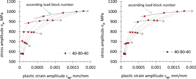
The dependence of the plastic strain and stress amplitude for a the increasing loading, b decreasing loading, in 40–80–40 type block loading
Fig. 15 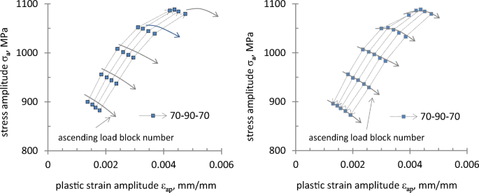
The dependence of the plastic strain and stress amplitude for a the increasing loading, b decreasing loading, in 70–90–70 type block loading


and
-
The plastic strain energy density expressed by the area of the hysteresis loop calculated as:
The history of value changes of the secant modulus Es is shown in Fig. 16a, while the plastic strain density ΔWpl is shown in Fig. 16b. Analyses were performed for loads of up to εamax < 2%. A decreasing value of secant modulus and an increasing value of plastic strain energy in successively repeated block loading make it possible to identify a distinct softening of Ti6Al4V alloy, regardless of the loading level. It can also be noticed that its properties tend to stabilize, whereas the stabilization is more distinct for lower levels of load. This is confirmed by a comparison of the ratios of plastic strain energy density calculated for particular levels of loading:
where:
- i:
-
number of the loading block.
Fig. 16 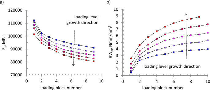
Changes of a secant modulus Es, b plastic strain energy density

Their values are presented in Fig. 17. The comparisons show that the value of R is higher for higher loading levels regardless of the number of loading blocks applied. The situation changes for higher strain values (3–4%), where the strain values are much less dependent on the number of applied loading blocks.

Plastic strain energy density ratios for particular loading levels
Such a variability of plastic strain makes it difficult to provide an unambiguous description of the material’s cyclic properties. Since one of the objectives of the tests was to analyze the distribution of the layered material’s local cyclic properties, the comparative analysis carried out was limited to the properties determined after the application of the same number of loading blocks to each specimen.
An analysis of the hysteresis loop parameters of the same loading block for each tested specimen made it possible to determine the K′ (cyclic strength coefficient) and n′ (cyclic strain hardening exponent) parameters for the Ramberg-Osgood model (1), disregarding the impact of cyclic instability of the tested materials. The values of K′ and n′ were determined on the basis of the process of stress amplitude changes σa in function of the plastic strain amplitude εa, according to dependence (2). The σa–εa relation for the aluminum alloy AA2519 (specimens A1–A5) are shown in Fig. 18a. Additionally, in Fig. 18a, there are diagrams of σa–εa determined for AA1050 aluminum with the use of transverse specimens. The results of Ti6Al4V (T7–T10) titanium alloy tests are presented in Fig. 18b. Like in static tests, specimens collected from the base materials and subjected to the same heat treatment as the layered material after the process of heating were also analyzed.

Stress amplitude vs. plastic strain curves, a AA2519 alloy, b Ti6Al4V alloy
The values of the parameters K′ and n′ determined for particular layers of AA2519-AA1050-Ti6Al4V material and base materials are presented in Fig. 19 and Table 10.

Distribution of local cyclic material properties
An analysis of the σa–εa dependence determined for each layer of AA2519 aluminum alloy revealed relatively small differences in the parameters n′ and K′. Maximal differences calculated in relation to their mean value did not exceed 6% for n′ and 9% for K′. Much bigger differences resulted from a comparison of their mean values with the parameters n′ and K′ determined for the base material subjected to the same heat treatment. In this case, the values of the parameters n′ and K′ are 36% and 16% lower, respectively (Table 10).
Such big differences can have a significant impact on estimation of the level of stress and strain in the layered material, for example, in numerical modeling. It applies particularly to the analysis of stress and strain distributions in fatigue analysis of a structure. Many methods of calculation of fatigue life are based on phenomenological descriptions of the process of fatigue damage summation in which the damage level caused by a single loading cycle is determined based on the analysis of local stresses and strains. Thus, even calculation errors of small value will result in significant underestimation or overestimation of fatigue life.
In the case of Ti6Al4V titanium alloy, the differences in the values of n′ and K′ for its particular layers are slightly higher than in the case of aluminum alloy; however, they do not exceed 17% for n′ and 6% for K′. The differences between the base material properties and the mean values of n′ and K′ calculated for a layer of Ti6Al4V are insignificant, being 15% for n′ and almost 5.5% for K′. Hence, it can be assumed that in this case, modeling of the layered material with the use of the base material properties does not have a significant influence on the determination of the value of local stress and strain.
To illustrate the differences between the determined cyclic properties, Fig. 20 shows the cyclic stress–strain curves described by Eq. (1), determined for particular layers of AA2519-AA1050-Ti6Al4V material.

Cyclic stress–strain curves
It should be noted that a description of the σa–εa relation with the use of the linear approximation, and thus a constant value of the cyclic strain hardening exponent n′ (2) does not represent the real properties of the analyzed titanium alloy (Fig. 21). Thus, the Ramberg-Osgood model (1) is not suitable to describe the material cyclic values within the whole range of plastic strains. In the case of both AA2519 and Ti6Al4V layers, their cyclic properties differ significantly from their static properties. Their comparison is shown in Fig. 22. For better clarity, the figure includes only static tension diagrams for specimens at macroscale and cyclic stress–strain curves for single layer. In the case of AA1050 alloy, the cyclic stress–strain curve is compared with the diagrams of static tension determined for a transverse specimen and a specimen of layer A6. Considering the cyclic instability of properties of alloys AA2519 and Ti6Al4V, Fig. 22 also shows the range of variability of cyclic properties. In the case of AA2519 alloy, cyclic loading causes material hardening reflected by an increase in the yield point along with an increase in its strength. The material hardening increases along with an increase in the number of applied loading blocks.

Linear approximation of stress amplitude–plastic strain amplitude curve

Comparison of static and cyclic stress–strain curves
In the case of Ti6Al4V alloy, the situation is more complicated. The comparison of static and cyclic properties shows that cyclic loading causes a gradual decrease in its yield point. In an earlier part of the study, the process of Ti6Al4V alloy softening along with an increase in the number of applied loading blocks is analyzed. However, independently of the decrease in the yield point, cyclic loading caused growth of its strength. The ultimate tensile strength determined in static tests was 950 MPa, and the level of stress amplitude determined in the loops exceeded 1100 MPa. The influence of the number of applied loading blocks is best seen in the range of total strain amplitudes from 0.5 to 2%.
A comparison of the cyclic stress–strain curve with the static tensile diagram for AA1050 alloy revealed a significant resemblance of the determined characteristics. Thus, it can be said that cyclic loading does not have a significant impact on its mechanical properties.
4 Conclusions
The study presents the results of tests of local mechanical properties of an explosively welded layered material AA2519-AA1050-Ti6Al4V. The tests were performed with the use of microspecimens collected from 10 parallel layers located parallel to the welding zone.
The tests were carried out under static and cyclic loads with the use of an MFS system for testing of microspecimens.
An analysis of the test results allows the following conclusions to be formulated:
-
1.
The distribution of static properties in the cross-section of the layered material does not indicate their significant diversification in particular layers.
-
2.
Explosion welding and heat treatment caused slight changes in the static properties of particular layers of the laminate in relation to the base materials. They mainly involved a slight softening, reflected by a decrease in the yield point for Ti6Al4V alloy and the yield point and ultimate tensile stress for AA2519.
-
3.
The distribution of microhardness along the transverse cross-section of the laminate is consistent with the distribution of static properties; however, analysis based on microhardness measurement can lead to their overestimation.
-
4.
The distribution of local cyclic properties, like the distribution of static properties, does not indicate their significant diversification in particular layers. However, in contrast to static loads, even small differences can be significant for a description of cyclic properties when they are used in fatigue analysis of a structure, for example in calculations of fatigue life on the basis of local distributions of stresses and strains.
-
5.
There was a distinct difference between the cyclic properties of particular layers of AA2519 alloy and the cyclic properties of the base material.
-
6.
The dependence of stress and plastic strain amplitude of Ti6Al4V alloy is of strongly nonlinear character, particularly in the range of higher values of plastic strains, and the effect is that the constant value of the cyclic strength coefficient n′ and cyclic strength coefficient K′ does not reflect the material’s real properties. Thus, the Ramberg-Osgood model based on it fails to describe exactly the results of tests of cyclic properties for Ti6Al4V alloy and should not be used for their description, especially if it was to be used for the entire range of plastic strains.
-
7.
Both the aluminum alloy AA2519 and the titanium alloy Ti6Al4V were characterized by cyclic instability. In the case of aluminum alloy, cyclic loading caused its cyclic hardening, whereas softening was found for titanium alloy with a simultaneous increase in its strength as compared with static loading.
Data availability
The raw/processed data required to reproduce these findings cannot be shared at this time due to technical limitations.
References
Eagar TW, Mazzeo AD (2011) Fundamentals of Fusion Welding, Welding Process Fundamentals, in: Lienert TJ, Babu SS, Siewert TA, Acoff VL (Eds.), ASM hHandbook, Vol. 6A, Weld. Fundam. Process., ASM International
Kurt B, Orhan N, Evin E, Çalik A (2007) Diffusion bonding between Ti-6Al-4V alloy and ferritic stainless steel. Mater Lett 61:1747–1750. https://doi.org/10.1016/j.matlet.2006.07.123
Saito Y, Utsunomiya H, Tsuji N, Sakai T (1999) Novel ultra-high straining process for bulk materials—development of the accumulative roll-bonding (ARB) process. Acta Mater 47:579–583. https://doi.org/10.1016/S1359-6454(98)00365-6
Ghalandari L, Mahdavian MM, Reihanian M (2014) Microstructure evolution and mechanical properties of Cu/Zn multilayer processed by accumulative roll bonding (ARB). Mater Sci Eng A 593:145–152. https://doi.org/10.1016/j.msea.2013.11.026
Akramifard HR, Mirzadeh H, Parsa MH (2014) Cladding of aluminum on AISI 304L stainless steel by cold roll bonding: mechanism, microstructure, and mechanical properties. Mater Sci Eng A 613:232–239. https://doi.org/10.1016/j.msea.2014.06.109
Dhib Z, Guermazi N, Ktari A, Gasperini M, Haddar N (2017) Mechanical bonding properties and interfacial morphologies of austenitic stainless steel clad plates. Mater Sci Eng A 696:374–386. https://doi.org/10.1016/j.msea.2017.04.080
Zhu Z, He Y, Zhang X, Liu H, Li X (2016) Effect of interface oxides on shear properties of hot-rolled stainless steel clad plate. Mater Sci Eng A 669:344–349. https://doi.org/10.1016/j.msea.2016.05.066
Xiao H, Qi Z, Yu C, Xu C (2017) Preparation and properties for Ti/Al clad plates generated by differential temperature rolling. J Mater Process Technol 249:285–290. https://doi.org/10.1016/j.jmatprotec.2017.06.013
Findik F (2011) Recent developments in explosive welding. Mater Des 32:1081–1093. https://doi.org/10.1016/j.matdes.2010.10.017
Grignon F, Benson D, Vecchio KS, Meyers MA (2004) Explosive welding of aluminum to aluminum: analysis, computations and experiments. Int J Impact Eng 30:1333–1351. https://doi.org/10.1016/j.ijimpeng.2003.09.049
Carvalho GHSFL, Mendes R, Leal RM, Galvão I, Loureiro A (2017) Effect of the flyer material on the interface phenomena in aluminium and copper explosive welds. Mater Des 122:172–183. https://doi.org/10.1016/j.matdes.2017.02.087
Mamalis AG, Vaxevanidis NM, Szalay A, Prohaszka J (1994) Fabrication of aluminium/copper bimetallics by explosive cladding and rolling. J Mater Process Technol 44:99–117. https://doi.org/10.1016/0924-0136(94)90042-6
Zhang N, Wang W, Cao X, Wu J (2015) The effect of annealing on the interface microstructure and mechanical characteristics of AZ31B/AA6061 composite plates fabricated by explosive welding. Mater Des 65:1100–1109. https://doi.org/10.1016/j.matdes.2014.08.025
Yan YB, Zhang ZW, Shen W, Wang JH, Zhang LK, Chin BA (2010) Microstructure and properties of magnesium AZ31B–aluminum 7075 explosively welded composite plate. Mater Sci Eng A 527:2241–2245. https://doi.org/10.1016/j.msea.2009.12.007
Aizawa Y, Nishiwaki J, Harada Y, Muraishi S, Kumai S (2016) Experimental and numerical analysis of the formation behavior of intermediate layers at explosive welded Al/Fe joint interfaces. J Manuf Process 24:100–106. https://doi.org/10.1016/j.jmapro.2016.08.002
SUN X, TAO J, GUO X (2011) Bonding properties of interface in Fe/Al clad tube prepared by explosive welding. Trans Nonferrous Metals Soc China 21:2175–2180. https://doi.org/10.1016/S1003-6326(11)60991-6
Balasubramanian V, Rathinasabapathi M, Raghukandan K (1997) Modelling of process parameters in explosive cladding of mildsteel and aluminium. J Mater Process Technol 63:83–88. https://doi.org/10.1016/S0924-0136(96)02604-0
Li X, Ma H, Shen Z (2015) Research on explosive welding of aluminum alloy to steel with dovetail grooves. Mater Des 87:815–824. https://doi.org/10.1016/j.matdes.2015.08.085
Gerland M, Presles H, Guin J, Bertheau D (2000) Explosive cladding of a thin Ni-film to an aluminium alloy. Mater Sci Eng A 280:311–319. https://doi.org/10.1016/S0921-5093(99)00695-4
Habib MA, Keno H, Uchida R, Mori A, Hokamoto K (2015) Cladding of titanium and magnesium alloy plates using energy-controlled underwater three layer explosive welding. J Mater Process Technol 217:310–316. https://doi.org/10.1016/j.jmatprotec.2014.11.032
Mamalis AG, Szalay A, Vaxevanidis NM, Pantelis DI (1994) Macroscopic and microscopic phenomena of nickel/titanium “shape-memory” bimetallic strips fabricated by explosive cladding and rolling. Mater Sci Eng A 188:267–275. https://doi.org/10.1016/0921-5093(94)90381-6
Topolski K, Wieciński P, Szulc Z, Gałka A, Garbacz H (2014) Progress in the characterization of explosively joined Ti/Ni bimetals. Mater Des 63:479–487. https://doi.org/10.1016/j.matdes.2014.06.046
Kahraman N, Gülenç B (2005) Microstructural and mechanical properties of Cu–Ti plates bonded through explosive welding process. J Mater Process Technol 169:67–71. https://doi.org/10.1016/j.jmatprotec.2005.02.264
Chu Q, Zhang M, Li J, Yan C (2017) Experimental and numerical investigation of microstructure and mechanical behavior of titanium/steel interfaces prepared by explosive welding. Mater Sci Eng A 689:323–331. https://doi.org/10.1016/j.msea.2017.02.075
Song J, Kostka A, Veehmayer M, Raabe D (2011) Hierarchical microstructure of explosive joints: example of titanium to steel cladding. Mater Sci Eng A 528:2641–2647. https://doi.org/10.1016/j.msea.2010.11.092
(1977) MIL-J-24445A(SH) MIL-J-24445 (SHIPS) Military specification joint, bimetallic bonded, aluminum to steel
Zeng X, Wang Y, Li X, Li X, Zhao T (2019) Effect of inert gas-shielding on the interface and mechanical properties of Mg/Al explosive welding composite plate. J Manuf Process 45:166–175. https://doi.org/10.1016/J.JMAPRO.2019.07.007
Yazdani M, Toroghinejad MR, Hashemi SM (2015) Investigation of microstructure and mechanical properties of St37 steel-Ck60 steel joints by explosive cladding. J Mater Eng Perform 24:4032–4043. https://doi.org/10.1007/s11665-015-1670-3
Xia H, Wang S, Ben H (2014) Microstructure and mechanical properties of Ti/Al explosive cladding. Mater Des 56:1014–1019. https://doi.org/10.1016/j.matdes.2013.12.012
Borchers C, Lenz M, Deutges M, Klein H, Gärtner F, Hammerschmidt M, Kreye H (2016) Microstructure and mechanical properties of medium-carbon steel bonded on low-carbon steel by explosive welding. Mater Des 89:369–376. https://doi.org/10.1016/j.matdes.2015.09.164
Zhang L-J, Pei Q, Zhang J-X, Bi Z-Y, Li P-C (2014) Study on the microstructure and mechanical properties of explosive welded 2205/X65 bimetallic sheet. Mater Des 64:462–476. https://doi.org/10.1016/J.MATDES.2014.08.013
Wang Z, Xiao Z, Tse Y, Huang C, Zhang W (2019) Optimization of processing parameters and establishment of a relationship between microstructure and mechanical properties of SLM titanium alloy. Opt Laser Technol 112:159–167. https://doi.org/10.1016/J.OPTLASTEC.2018.11.014
Zhang H, Jiao KX, Zhang JL, Liu J (2018) Microstructure and mechanical properties investigations of copper-steel composite fabricated by explosive welding. Mater Sci Eng A 731:278–287. https://doi.org/10.1016/J.MSEA.2018.06.051
Parchuri P, Kotegawa S, Yamamoto H, Ito K, Mori A, Hokamoto K (2019) Benefits of intermediate-layer formation at the interface of Nb/Cu and Ta/Cu explosive clads. Mater Des 166:107610. https://doi.org/10.1016/J.MATDES.2019.107610
Yang M, Ma H, Yao D, Shen Z (2019) Experimental study for manufacturing 316L/CuCrZr hollow structural component. Fusion Eng Des 144:107–118. https://doi.org/10.1016/J.FUSENGDES.2019.04.090
Gladkovsky SV, Kuteneva SV, Sergeev SN (2019) Microstructure and mechanical properties of sandwich copper/steel composites produced by explosive welding. Mater Charact 154:294–303. https://doi.org/10.1016/J.MATCHAR.2019.06.008
Zeng X, Wang Y, Li X, Li X, Zhao T (2019) Effects of gaseous media on interfacial microstructure and mechanical properties of titanium/steel explosive welded composite plate. Fusion Eng Des 148:111292. https://doi.org/10.1016/J.FUSENGDES.2019.111292
Fronczek DM, Wojewoda-Budka J, Chulist R, Sypien A, Korneva A, Szulc Z, Schell N, Zieba P (2016) Structural properties of Ti/Al clads manufactured by explosive welding and annealing. Mater Des 91:80–89. https://doi.org/10.1016/j.matdes.2015.11.087
Corigliano P, Crupi V, Guglielmino E (2018) Non linear finite element simulation of explosive welded joints of dissimilar metals for shipbuilding applications. Ocean Eng 160:346–353. https://doi.org/10.1016/J.OCEANENG.2018.04.070
Kamaya M (2016) Ramberg–Osgood type stress–strain curve estimation using yield and ultimate strengths for failure assessments. Int J Press Vessel Pip 137:1–12. https://doi.org/10.1016/J.IJPVP.2015.04.001
Skelton RP, Maier HJ, Christ H-J (1997) The Bauschinger effect, Masing model and the Ramberg–Osgood relation for cyclic deformation in metals. Mater Sci Eng A 238:377–390. https://doi.org/10.1016/S0921-5093(97)00465-6
Ramberg W, Osgood WR, (1943) Description of stress-strain curves by three parameters. Natl Advis Comm. Aeronaut. Tech. Note No. 902
Jones A, Hudd R (1999) Cyclic stress-strain curves generated from random cyclic strain amplitude tests. Int J Fatigue 21:521–530. https://doi.org/10.1016/S0142-1123(99)00014-6
Boroński D (2006) Cyclic material properties distribution in laser-welded joints. Int J Fatigue 28:346–354. https://doi.org/10.1016/J.IJFATIGUE.2005.07.029
Neuber H (1961) Theory of stress concentration for shear-strained prismatical bodies with arbitrary nonlinear stress-strain law. ASME J Appl Mech 28:544–550
Molski K, Glinka G (1981) A method of elastic-plastic stress and strain calculation at a notch root. Mater Sci Eng 50:93–100
Glinka G (1985) Energy density approach to calculation of inelastic strain-stress near notched and cracks. Eng Fract Mech 22:485–508
Szachogluchowicz I, Sniezek L, Hutsaylyuk V (2016) Low cycle fatigue properties of AA2519–Ti6Al4V laminate bonded by explosion welding. Eng Fail Anal 69:77–87. https://doi.org/10.1016/j.engfailanal.2016.01.001
Bazarnik P, Adamczyk-Cieślak B, Gałka A, Płonka B, Snieżek L, Cantoni M, Lewandowska M, (2016) Mechanical and microstructural characteristics of Ti6Al4V/AA2519 and Ti6Al4V/AA1050/AA2519 laminates manufactured by explosive welding, 111 146–157. http://www.sciencedirect.com/science/article/pii/S0264127516311510 (accessed May 19, 2017)
Gałka A (2015) Application of explosive metal cladding in manufacturing new advanced layered materials on the example of titanium Ti6Al4V – aluminum AA2519 bond. High-Energetic Mater 7:73–79
Boroński D, Kotyk M, Maćkowiak P, Śnieżek L (2017) Mechanical properties of explosively welded AA2519-AA1050-Ti6Al4V layered material at ambient and cryogenic conditions. Mater Des 133:390–403. https://doi.org/10.1016/j.matdes.2017.08.008
Boroński D (2015) Testing low-cycle material properties with micro-specimens. Mater Test 57:165–170. https://doi.org/10.3139/120.110693
Boroński D (2012) Material properties investigations with the use of microspecimen. Mater Sci Forum 726:51–54. https://doi.org/10.4028/www.scientific.net/MSF.726.51
Boroński D, Sołtysiak R, Giesko T, Marciniak T, Lutowski Z, Bujnowski S, (2014) The investigations of fatigue cracking of laser welded joint with the use of “FatigueVIEW” system Key Eng Mater. 598. https://doi.org/10.4028/www.scientific.net/KEM.598.26
Hickey JCF Tensile strength-hardness correlation for titanium alloys. ASTM Proc 61(1961):857–865
Keist JS, Palmer TA (2017) Development of strength-hardness relationships in additively manufactured titanium alloys. Mater Sci Eng A 693:214–224. https://doi.org/10.1016/J.MSEA.2017.03.102
Tiryakioğlu M, Robinson JS, Salazar-Guapuriche MA, Zhao YY, Eason PD (2015) Hardness–strength relationships in the aluminum alloy 7010. Mater Sci Eng A 631:196–200. https://doi.org/10.1016/J.MSEA.2015.02.049
Tiryakioğlu M (2015) On the relationship between Vickers hardness and yield stress in Al–Zn–Mg–Cu alloys. Mater Sci Eng A 633:17–19. https://doi.org/10.1016/J.MSEA.2015.02.073
Stathers PA, Hellier AK, Harrison RP, Ripley MI, Norrish J (2014) Hardness-tensile property relationships for HAZ in 6061-T651 aluminum. Weld J 93:301–311 https://ro.uow.edu.au/eispapers/2846 (accessed November 15, 2019)
Khodabakhshi F, Haghshenas M, Eskandari H, Koohbor B (2015) Hardness−strength relationships in fine and ultra-fine grained metals processed through constrained groove pressing. Mater Sci Eng A 636:331–339. https://doi.org/10.1016/J.MSEA.2015.03.122
Sato S, Endo T (1986) Relation between tensile strength and hardness of aluminum alloys. J Japan Inst Light Met 36:29–35. https://doi.org/10.2464/jilm.36.29
Funding
The explosively welded AA2519-AA1050-Ti6Al4V layered material was developed under the grant No. PBS2/A5/35/2013 of The National Centre for Research and Development of Poland.
Author information
Authors and Affiliations
Corresponding author
Additional information
Publisher’s note
Springer Nature remains neutral with regard to jurisdictional claims in published maps and institutional affiliations.
Recommended for publication by Commission IX - Behaviour of Metals Subjected to Welding
Rights and permissions
Open Access This article is licensed under a Creative Commons Attribution 4.0 International License, which permits use, sharing, adaptation, distribution and reproduction in any medium or format, as long as you give appropriate credit to the original author(s) and the source, provide a link to the Creative Commons licence, and indicate if changes were made. The images or other third party material in this article are included in the article's Creative Commons licence, unless indicated otherwise in a credit line to the material. If material is not included in the article's Creative Commons licence and your intended use is not permitted by statutory regulation or exceeds the permitted use, you will need to obtain permission directly from the copyright holder. To view a copy of this licence, visit http://creativecommons.org/licenses/by/4.0/.
About this article

Cite this article
Boroński, D. Local mechanical properties of explosively welded AA2519-AA1050-Ti6Al4V layered material. Weld World 64, 2083–2099 (2020). https://doi.org/10.1007/s40194-020-00984-2
Received:
Accepted:
Published:
Issue Date:
DOI: https://doi.org/10.1007/s40194-020-00984-2