
Abstract
One-dimensional (1D) model atmospheres are still the most commonly used tool for the determination of stellar chemical composition. Convection in the model is usually treated by mixing-length theory (MLT). The mixing-length parameter α is generally calibrated from the Sun and applied to all other stars. The metal-poor giant, HD 122563, is an important benchmark star to test stellar atmosphere and interior physics. We investigate the influence of the convection mixing-length parameter α on the determination of chemical abundances of Na, Mg, Al, Si, Ca, Sc, Ti, Cr, Mn, Co, Ni, Sr, Y, Zr and Ba in the case of HD 122563, taking advantage of a high resolution and high signal-to-noise ratio HARPS spectrum. The abundance discrepancies Δ[X/H] that occur due to α variation rarely exceed 0.05 dex and most are less than 0.03 dex. We calculate the discrepancy Δ[X/H] using a line-by-line differential analysis. The abundance discrepancies do not have direct relation with either line strength or the excitation potential. For 1D stellar atmospheric analysis of HD 122563, the accuracy of abundance determination does not strongly depend on the choice of mixing-length parameter α (causing average discrepancies of < 0.03 dex), while the uncertainties in the effective temperature and surface gravity play a more important role.
Export citation and abstract BibTeX RIS
1. Introduction
The determination of stellar abundances plays an integral part in our quest to understand stellar, galactic and cosmic evolution. The derivation of accurate element abundances requires realistic models of the stellar atmospheres. Still today, the vast majority of abundance analyses of late-type stars rely on one-dimensional (1D) hydrostatic model atmospheres, such as ATLAS (Kurucz 1993; Castelli & Kurucz 2003), MARCS (Gustafsson et al. 2008) and MAFAGS-OS (Grupp 2004a,b). The convection in stellar envelopes is one of the largest sources of uncertainty in the interior modeling of stars. Convective heat transport is widely treated by the classical mixing-length theory (MLT; Böhm-Vitense 1958) and some close relative thereof (Canuto & Mazzitelli 1991, 1992).
The mixing-length parameter α is a free parameter that represents the efficiency of convection in MLT. Usually this parameter is calibrated on the Sun (Henyey et al. 1965; Bernkopf 1998). Because there are not enough calibration stars to determine the α value through precise stellar parameters except the Sun, most stellar models generally treat convection in stellar envelopes with MLT adopting the universal solar-calibrated α value. Indeed, it is now known that assuming all stars should have the same α as the solar-calibrated value is incorrect. New α values were recalibrated for nearby bright stars through observations, such as for α Cen AB (Guenther & Demarque 2000), Procyon A (Straka et al. 2005) and 16 Cyg AB (Metcalfe et al. 2012). Bonaca et al. (2012) calculated α for many other stars in the Kepler field with asteroseismic data. However, these recalibrated α values mostly are based on accurate asteroseismology data, which thus have limited the range of application and can only apply to specific samples. Recently, three-dimensional (3D) radiative hydrodynamic simulations of atmospheric models have achieved great improvement, e.g., CO5BOLD (Freytag et al. 2012) and STAGGER (Magic et al. 2013). Several studies focused on calibrating mixing-length parameter α by matching averages of the 3D radiative hydrodynamic simulations to 1D stellar envelope models (Trampedach et al. 2014; Magic et al. 2015). This method allows the α value of a specific star with properties different from the Sun to be predicted through a grid of 3D models for a set of effective temperature (Teff), surface gravity (log g) and metallicity ([M/H]).
The relationship between convection and the stellar properties (Teff, log g and [M/H]) has been studied in a number of works. Both observational data (Viani et al. 2018) and theoretical simulations (Valle et al. 2019) were applied to investigate the relation between α and stellar atmospheric parameters. Some works have focused on stellar metallicity which was important for shedding light on the history of the cosmos. The observational study of Bonaca et al. (2012) and theoretical work of Tanner et al. (2013) both suggested that the stellar surface convection depends on the chemical composition of the convective envelope. Specific star samples were used for detailed investigations as well. Collet et al. (2007) and Kučinskas et al. (2013) employed 3D simulations of stellar surface convection in red giant stars to study the impact on spectral line formation and abundance analysis. These authors pointed out the differences between abundance determinations based on 3D and 1D models are particularly large at low metallicities. In our previous study (Song et al. 2020), we quantified the impact of the mixing-length parameter α on the discrepancy of iron abundance (Δ[Fe/H]) with high-quality spectral data for two well-studied samples. We found that the low metallicity giant stars demonstrated a larger Δ[Fe/H] caused by varying the value of α. Besides iron abundance, we also need to evaluate the effect of convective mixing length parameters α on the abundances of other elements.
The brightest known metal-poor halo giant star, HD 122563 (V = 6.2 mag, [Fe/H] ≈ –2.6) has been the subject of numerous spectroscopic analyses (e.g., Aoki et al. 2007; Afşar et al. 2016; Prakapavičius et al. 2017; Collet et al. 2018). Thanks to its close distance to the Sun (3.44mas; Gaia Collaboration et al. 2018), HD 122563 has been measured utilizing various methodologies given the new high precision instruments, which has made it an important astrophysical laboratory to test stellar atmospheric and interior physics. For the above-listed reasons, HD 122563 is an ideal object for estimating the influence of convective mixing length α on abundance determination. We aim to study abundance discrepancy caused by α value variation for metallic lines in HD 122563.
The paper is organized as follows. Section 2 introduces the source spectrum, model calculation and analysis method. Section 3 presents the results and discussion. We elaborate upon the impact of α on abundance determination and compare with the impact of other atmospheric parameters (Teff, log g). Section 4 gives our conclusions and prospects for future work.
2. Observed and Synthetic Spectra
2.1. High-quality Spectrum from HARPS
In order to achieve sufficient precision and accuracy to determine the influence of α on line formation through the spectral synthesis method, observed spectra with high quality become critical. High Accuracy Radial velocity Planet Searcher (HARPS) (Mayor et al. 2003) at the European Southern Observatory (ESO) La Silla 3.6 m telescope observed stars with high resolution and high signal-to-noise ratio in order to search for exoplanets. Most of the nearby, bright stars were observed by HARPS. The resolution of spectra observed by HARPS is R ∼ 115 000. ESO has continued to release all HARPS science data in HAM/EGGS modes since the beginning of instrument operation in October 2003. All the released data are easily searched, checked and downloaded through the ESO Archive Science Portal1
We selected the spectrum with highest signal-to-noise ratio (S/N = 318.5) of HD 122563 observed by HARPS. The spectrum was obtained on 2008 February 24 with exposure of 1500 s. This spectrum had been reduced automatically using the Data Reduction Software (DRS) pipeline developed by the HARPS Consortium. The spectrum ranges from 3800 Å to 6900 Å, which covers several strong metallic lines for our analysis. There is one spectral order (N = 115, from 5300 Å to 5330 Å) that was lost due to a gap between two CCD chips, which should, however, not affect our analysis,
2.2. Stellar Atmospheric Parameters
In order to produce the stellar model grids of HD 122563, the basic stellar atmospheric parameters including effective temperature and surface gravity were derived through the following method. Effective temperature Teff was obtained by fitting the wings of Balmer lines, Hα and Hβ. This analysis is based on the non-local thermodynamic equilibrium (NLTE) line formation for Hi implementing the method described in Mashonkina et al. (2008). Theoretical NLTE Hα and Hβ line profiles were calculated with the code Spectrum Investigation Utility (SIU) (Reetz 1999) with the departure coefficients calculated with a revised version of the code DETAIL (Butler & Giddings 1985). The updates are described in Mashonkina et al. (2008). The absorption profiles of Balmer lines were convolved with thermal, natural and Stark broadening, as well as self-broadening. For self-broadening, the Lorentz profile with a half-width computed considering the cross-section and velocity parameter from Barklem et al. (2000) was applied. In Figure 1 we display the fitting profiles of Hα and Hβ with the final Teff. We derived the final effective temperature Teff = 4600 ± 50 K which is consistent with previous study (Mashonkina et al. 2011).
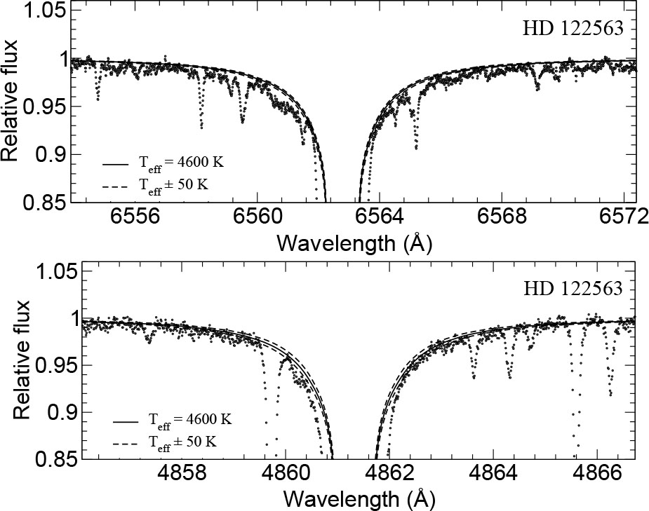
Fig. 1 Hα and Hβ wing profile fitting of HD 122563 to determine Teff.
Download figure:
Standard imageThe surface gravity log g was estimated based on the latest and more precise parallax of 3.444 ± 0.063 mas, which was adopted from the Gaia Data Release 2 (DR2) catalog (Gaia Collaboration et al. 2018). The bolometric corrections for the absolute bolometric magnitude were taken from Alonso et al. (1999). We derived a final surface gravity log g of 1.40 ± 0.05 which is in good agreement with literature values such as Creevey et al. (2019)
2.3. New Mixing-length Parameter α
As usual, during the modeling of stellar structure and evolution, the solar value of α was adopted, despite the diverse properties of stellar atmospheres. We need to calibrate the new α to replace the unified solar α for our sample in order to meet our analysis requirement.
3D theoretical model atmospheres in Magic et al. (2015) covered a wide range in stellar parameter space. Their paper performed functional fits of the mixing-length parameter f(x,y) with Teff and log g for different metallicities individually. We have employed the model to predict the standard MLT α by Böhm-Vitense (1958, formulation in a 1D model. The stellar parameters were transformed with x = (Teff – 5777)/1000 and y = log g – 4.44. The fitting function is
The coefficients ai are listed in Table B.1 in Magic et al. (2015) for a grid of different metallicities. The ai were calculated by interpolation for each star. The new α value of HD 122563 fitted from Equation (1) was αBV = 2.0. Wu et al. (2015) used Balmer-line fitting and spectral energy distribution (SED) fits to determine the recalibrated α for several stars and derived αCM = 1.0 for HD 122563, which was suitable for the Canuto & Mazzitelli (1991, 1992, CM hereafter) formulation. We finally adopted 2.0, which is based on the more common BV theory, as our input α value for the benchmark model. In the following analysis, the α of CM theory was also applied to calculate a grid of models. We compared the difference in abundances due to the two different α values.
2.4. Grid of Stellar Models
The analysis was performed using plane-parallel, homogeneous (1D) local thermodynamic equilibrium (LTE) model atmospheres calculated with the code MAFAGS-OS (Grupp 2004a,b). MAFAGS-OS provides flexible selection of input parameters, which enabled us to perform the calculations with different atmospheric parameter grids. More importantly, this code allows for adjusting mixing-length parameter α with both BV and CM theory to treat convection.
Based on the Teff and log g derived in Section 2.2 and new α value in Section 2.3, we calculated a grid of models to cover the steps of Teff, log g and α individually for HD 122563. The details of the grid models are summarized in Table 1. We separate these models into six groups. Group 0 stands for the basic model with the stellar parameters that we adopt for HD 122563 (Teff = 4600 K, log g = 1.40, [Fe/H] = –2.6, α = 2.0). This model was regarded as a standard benchmark. All the other models in the following groups were compared with this one to derive the abundance discrepancy. In the other five Groups, we calculated a grid with reasonable step sizes of one parameter and kept the other two parameters consistent with Group 0. The highest α was determined as 2.5. Higher values do not satisfy the MLT theory and the real physical picture. Group 4 and Group 5 were calculated with αCM in order to investigate the difference between the two MLT α theories.
Table 1. Grid of Stellar Models
| Group | Grid | Teff (K) | log g (dex) | α (dex) | N |
|---|---|---|---|---|---|
| 0 | basic | 4600 | 1.43 | 2.0 (αBV) | 1 |
| 1 | αBV | - | - | 0.5, 1.0, 1.5, 2.5 | 4 |
| 2 | Δ log g | - | ±0.05, ±0.1, ±0.2 | - | 6 |
| 3 | Δ Teff | ±50, ±100 | - | - | 4 |
| 4 | αCM | - | - | 1.0 (αCM) | 1 |
| 5 | αCM | - | - | 0.5, 1.5, 2.0, 2.5 | 4 |
aTotal number of stellar models used in the corresponding group.
Table 2. Average Abundance Discrepancies in Different Stellar Model Grids
| Species | |Δ[X/H]αBV| | ![$\overline{\Delta {[{\rm{X}}/{\rm{H}}]}_{\mathrm{log}g}}$](https://content.cld.iop.org/journals/1674-4527/20/8/121/revision1/raa_20_8_121_ieqn1.gif) |
![$\overline{\Delta {[{\rm{X}}/{\rm{H}}]}_{{T}_{{\rm{eff}}}}}$](https://content.cld.iop.org/journals/1674-4527/20/8/121/revision1/raa_20_8_121_ieqn2.gif) |
N |
||||||
|---|---|---|---|---|---|---|---|---|---|---|
| –1.5 | –1.0 | –0.5 | +0.5 | 0.2 | 0.1 | 0.05 | 100 K | 50 K | ||
| Nai | 0.020 | 0.020 | 0.030 | 0.010 | 0.090 | 0.045 | 0.020 | 0.185 | 0.085 | 2 |
| Mgi | 0.016 | 0.016 | 0.016 | 0.006 | 0.106 | 0.054 | 0.026 | 0.126 | 0.062 | 5 |
| Ali | — | — | 0.040 | 0.010 | 0.100 | 0.050 | 0.020 | 0.140 | 0.070 | 1 |
| Sii | — | — | 0.040 | 0.010 | 0.090 | 0.050 | 0.025 | 0.095 | 0.035 | 2 |
| Cai | 0.022 | 0.018 | 0.022 | 0.007 | 0.077 | 0.037 | 0.018 | 0.108 | 0.055 | 6 |
| Scii | — | — | 0.005 | 0.035 | 0.025 | 0.010 | 0.005 | 0.040 | 0.020 | 2 |
| Tii | 0.024 | 0.014 | 0.020 | 0.011 | 0.070 | 0.033 | 0.015 | 0.145 | 0.075 | 6 |
| Tiii | 0.019 | 0.022 | 0.013 | 0.017 | 0.020 | 0.011 | 0.003 | 0.026 | 0.011 | 15 |
| Cri | 0.000 | 0.010 | 0.006 | 0.018 | 0.124 | 0.060 | 0.030 | 0.180 | 0.098 | 5 |
| Mni | — | — | 0.025 | 0.013 | 0.138 | 0.070 | 0.035 | 0.157 | 0.078 | 4 |
| Coi | — | — | 0.020 | 0.005 | 0.090 | 0.045 | 0.025 | 0.160 | 0.080 | 2 |
| Nii | 0.030 | 0.030 | 0.027 | 0.020 | 0.093 | 0.047 | 0.023 | 0.167 | 0.083 | 3 |
| Srii | — | — | 0.020 | 0.010 | 0.060 | 0.030 | 0.020 | 0.070 | 0.030 | 1 |
| Yii | — | — | 0.040 | 0.010 | 0.010 | 0.000 | 0.000 | 0.070 | 0.030 | 1 |
| Zrii | — | — | 0.030 | 0.000 | 0.020 | 0.010 | 0.000 | 0.020 | 0.010 | 1 |
| Baii | 0.017 | 0.023 | 0.023 | 0.003 | 0.040 | 0.023 | 0.007 | 0.083 | 0.043 | 3 |
| Total | 0.019 | 0.019 | 0.024 | 0.012 | 0.072 | 0.036 | 0.017 | 0.111 | 0.054 | 59 |
2.5. Line Selection and Atomic Data
The lines adopted in our research were selected from the lists of several abundance analysis papers (Mashonkina et al. 2010; Zhao et al. 2016; Aoki et al. 2018). These papers provided a suitable metallic line list in the optical wavelength range for metal-poor stars, which could be applied to HD 122563. Most reliable and up-to-date atomic input data were adopted from the NIST ASD2 as well as the above-mentioned references. The species identification, wavelength, excitation potential and gf values are included in Table 3. It should be noted that inaccurate atomic data could lead to unreliable derived abundances. However, in our study, we focus more on the abundance discrepancy due to the α influence instead of absolute abundance determination. Our analysis could counteract the uncertainty introduced by atomic data to a certain extent and thus the final result does not depend on the input atomic data.
2.6. Synthetic Spectra and the Abundance Discrepancy Calculation
Accurate line formation computations and abundance determination were performed with SIU. First we reprocessed the HARPS spectrum of HD 122563. The wavelength was recalibrated and flux normalization was performed manually in a 5 Å window for each individual line. We also recalibrated the wavelength of the spectrum to match the laboratory wavelength. We utilized the spline function for continuum rectification.
We applied SIU to calculate line profiles with selected stellar atmospheric models and produced synthetic spectra which overlap with the observed spectrum. To determine the abundance, we degrade the theoretical profiles with observational uncertainties by convolving them with a profile that combines instrumental broadening with a Gaussian profile, rotational broadening and broadening by macroturbulence with a radial-tangential profile. Finally, the best line profile and abundance were determined through adjusting the element abundance by minimizing the χ2 between the observed and synthetic spectra. Figure 2 presents an example of the best synthetic spectrum fit to the Cai λ6162 Å line calculated by SIU with benchmark model Group 0. We also evaluated the equivalent width for each line with SIU. During the spectral synthesis calculation, we eliminated bad lines, for example, heavily blended lines that are nearly unseparable and lines too weak to measure with high accuracy. The equivalent widths and abundances derived with the basic model (Group 0) for each line are presented in Table 3.
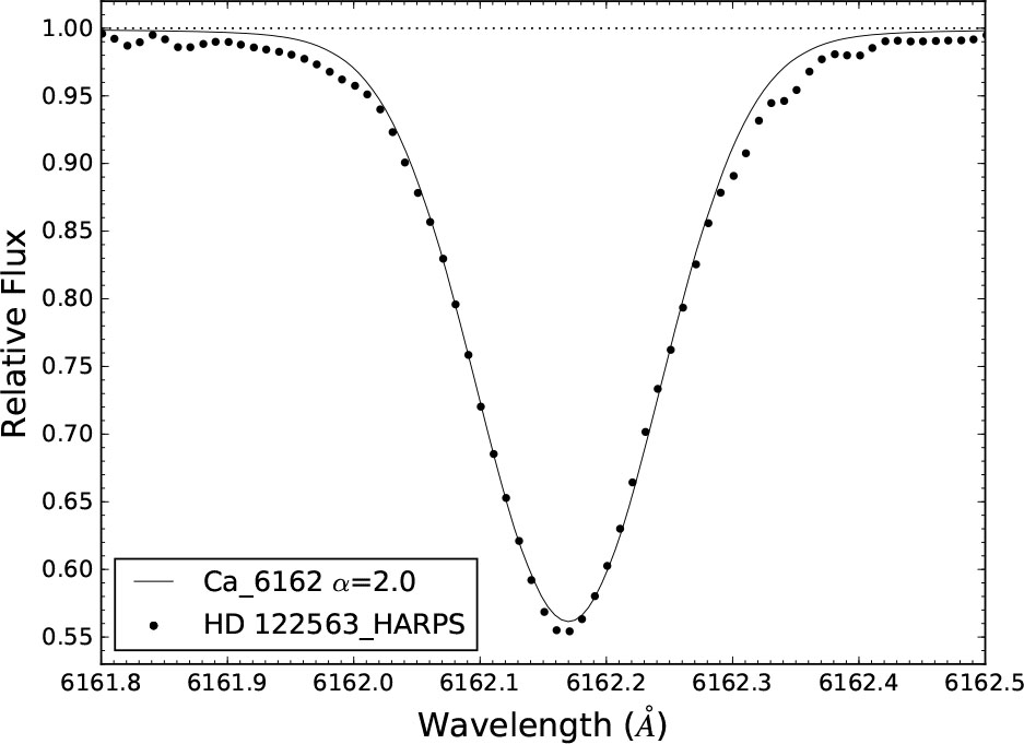
Fig. 2 Example of fitting the synthetic spectra of λ6162 Å with the observed spectrum. The new αBV = 2.0 was adopted.
Download figure:
Standard imageTable 3. Atomic line data, equivalent widths (EWs) and derived abundances for each metallic line.
| Species | λ Å | Eexc eV | log gf | EW mÅ | log  |
|---|---|---|---|---|---|
| Nai | 5889.96 | 0.00 | 0.11 | 178.7 | 4.29 |
| Nai | 5895.93 | 0.00 | –0.19 | 159.6 | 4.29 |
| Mgi | 4571.09 | 0.00 | –5.40 | 79.7 | 5.51 |
| Mgi | 4702.99 | 4.35 | –0.46 | 72.7 | 5.44 |
| Mgi | 5172.68 | 2.71 | –0.39 | 226.2 | 5.64 |
| Mgi | 5183.60 | 2.71 | –0.17 | 252.8 | 5.64 |
| Mgi | 5528.41 | 4.35 | –0.51 | 76.5 | 5.44 |
| Ali | 3961.52 | 0.01 | –0.33 | 156.8 | 3.96 |
| Sii | 3905.53 | 1.91 | –1.10 | 200.4 | 5.73 |
| Sii | 4102.94 | 1.91 | –2.99 | 80.9 | 5.63 |
| Cai | 4226.73 | 0.00 | 0.24 | 258.2 | 4.09 |
| Cai | 4454.78 | 1.94 | 0.26 | 75.6 | 4.28 |
| Cai | 5588.75 | 2.53 | 0.36 | 47.8 | 3.88 |
| Cai | 6122.22 | 1.89 | –0.32 | 67.7 | 4.19 |
| Cai | 6162.17 | 1.90 | –0.09 | 82.8 | 4.25 |
| Cai | 6439.08 | 2.53 | 0.39 | 63.6 | 4.08 |
| Scii | 4246.82 | 0.32 | 0.24 | 125.3 | 1.45 |
| Scii | 4415.56 | 0.60 | –0.67 | 80.1 | 1.20 |
| Tii | 3998.64 | 0.05 | –0.06 | 72.7 | 2.76 |
| Tii | 4533.25 | 0.85 | 0.48 | 50.8 | 2.47 |
| Tii | 4534.78 | 0.84 | 0.28 | 42.8 | 2.51 |
| Tii | 4981.73 | 0.85 | 0.51 | 59.3 | 2.63 |
| Tii | 4991.06 | 0.84 | 0.45 | 55.8 | 2.63 |
| Tii | 5210.39 | 0.05 | –0.88 | 44.3 | 2.43 |
| Tiii | 4028.34 | 1.89 | –0.96 | 49.8 | 2.83 |
| Tiii | 4394.05 | 1.22 | –1.78 | 62.1 | 2.53 |
| Tiii | 4395.03 | 1.24 | –1.93 | 50.4 | 2.73 |
| Tiii | 4399.77 | 1.24 | –1.19 | 90.8 | 2.73 |
| Tiii | 4417.72 | 1.16 | –1.19 | 93.9 | 3.32 |
| Tiii | 4418.33 | 1.24 | –1.97 | 50.8 | 3.35 |
| Tiii | 4443.79 | 1.08 | –0.72 | 120.2 | 2.83 |
| Tiii | 4444.56 | 1.12 | –2.24 | 48.2 | 2.80 |
| Tiii | 4450.48 | 1.08 | –1.52 | 86.7 | 3.43 |
| Tiii | 4464.45 | 1.16 | –1.81 | 69.5 | 2.78 |
| Tiii | 4468.51 | 1.13 | –0.60 | 127.4 | 2.73 |
| Tiii | 4470.86 | 1.16 | –2.02 | 50.2 | 2.73 |
| Tiii | 4501.27 | 1.12 | –0.77 | 107.3 | 3.23 |
| Tiii | 4533.97 | 1.24 | –0.53 | 100.6 | 2.66 |
| Tiii | 4571.97 | 1.57 | –0.32 | 113.3 | 2.71 |
| Cri | 4254.33 | 0.00 | –0.11 | 112.6 | 3.40 |
| Cri | 4274.80 | 0.00 | –0.23 | 108.2 | 3.45 |
| Cri | 4289.72 | 0.00 | –0.37 | 104.2 | 3.50 |
| Cri | 5206.04 | 0.94 | 0.02 | 88.3 | 3.15 |
| Cri | 5208.42 | 0.94 | 0.17 | 92.6 | 3.15 |
| Mni | 4030.75 | 0.00 | –0.47 | 132.8 | 3.70 |
| Mni | 4033.06 | 0.00 | –0.62 | 125.6 | 3.68 |
| Mni | 4034.48 | 0.00 | –0.81 | 112.9 | 3.62 |
| Mni | 4041.35 | 2.11 | 0.28 | 42.7 | 3.65 |
| Coi | 4118.77 | 1.05 | –0.47 | 78.2 | 3.00 |
| Coi | 4121.31 | 0.92 | –0.30 | 89.3 | 3.20 |
| Nii | 3807.14 | 0.42 | –1.22 | 111.1 | 4.22 |
| Nii | 3858.29 | 0.42 | –0.95 | 116.6 | 4.38 |
| Nii | 5476.90 | 1.83 | –0.89 | 79.9 | 3.62 |
| Srii | 4077.72 | 0.00 | 0.15 | 170.5 | 0.70 |
| Yii | 3950.35 | 0.10 | 0.49 | 48.1 | –0.08 |
| Zrii | 3998.97 | 0.56 | –0.52 | 40.1 | 0.30 |
| Baii | 4554.03 | 0.00 | 0.17 | 93.8 | –0.20 |
| Baii | 4934.07 | 0.00 | –0.15 | 88.3 | –0.20 |
| Baii | 6141.71 | 0.70 | –0.08 | 42.3 | –1.00 |
After deriving the synthetic spectrum of each line with the benchmark model, we employed other models in Group 1 to derive the abundances with different α values. Finally, the abundance discrepancy was derived. The abundance discrepancy due to αBV variation was defined as Δ [X/H]αBV = [X/H]αGroup1 – [X/H]αBV = 2.0. Here, the α value in Group 1 was 0.5, 1.0, 1.5 and 2.0 as we introduce in Section 2.4. We used similar definitions for Δ [X/H]Teff and Δ [X/H]log g to represent the impact of Teff and log g on abundance determination (Groups 2 and 3). We also calculated Δ [X/H]αCM which implemented another MLT of CM formulation for comparison (Groups 4 and 5). The final Δ [X/H] was derived with line-by-line differential analysis. We analyzed the metallicity discrepancy for several iron lines both under LTE and NLTE assumptions in our previous work (Song et al. 2020). Even though some line profiles could be fitted better under the NLTE assumption, the influence of convection on NLTE effects could be ignored with the line-by-line differential analysis, so we did not take NLTE effects into account in this work.
3. Results and Discussion
3.1. Influence of αBV on Abundance Determination
Based on the line list in Section 2.5, we analyzed 59 metallic lines for the following species to evaluate the influence of α on abundance determination:
- –neutral atoms: Nai, Mgi, Ali, Sii, Cai, Tii, Cri, Mni, Coi, Nii;
- –ionized atoms: Scii, Tiii, Srii, Yii, Zrii, Baii.
All these lines were thoroughly studied for the metal-poor giant HD 122563. In order to derive the best fitting profile for each line, the additional tunable broadening parameters were convolved by a Gaussian function for each input model. The abundance discrepancy of each line is listed in Table 4 in the columns marked by Group 1-0. The largest Δ [X/H]αBV values are 0.05 dex (Cai λ4226 Å with α = 0.5 and Scii λ4246 Å with α = 2.5). Most of the Δ [X/H]αBV values are lower than 0.04 dex, which suggest that the variation in α only results in a negligible degree of difference in abundances derived from metallic lines.
We also investigated the impact of α on the shape of the line profile (Fig. 3). The wings and core of weak lines are both formed in deep layers, where convection affects the wings and core in the same way. For weaker lines with equivalent widths less than 150 mÅ, α influences on the whole line profile are equal and there are no changes in the line shape of the final best fitted synthetic spectra after abundance rectification. For stronger lines, the core forms in layers shallower than those that form the wings, so convection influences the wings and core of the strong lines differently. The effects of α mostly influence the wings more than core of the line profile. However, it hardly affects the final abundance determination.

Fig. 3 Example of mixing-length parameter α influences on line profile. The synthetic spectra of strong line Ca λ4226 Å and weak line Ca λ4454 Å are plotted with three different α values. All the other stellar parameters of the three synthetic spectra are identical for each line. For the strong line λ4226 Å, we could identify the shape changes in the wings due to α variation, especially for α = 2.5. The impact of α on the weak line λ4554 Å is not obvious.
Download figure:
Standard imageWhen deriving abundances from absorption lines, it is assumed that the line strength is directly related to the abundance of the element. We plot the Δ [X/H]αBV versus equivalent width in order to investigate the influence of α on the strength of the line (Fig. 4). For the metal-poor star HD 122563, most of the lines are weak. Only limited lines (e.g., Mg Ib, Na D) are strong lines. There is no obvious relationship between line strength and abundance discrepancy. Both neutral lines and ionized lines experience little change in HD 122563.

Fig. 4 Abundance discrepancy caused by α variation for all the metallic lines, plotted versus the equivalent width of each line. The neutral and singly ionized atoms are identified separately. The models with αBV = 0.5, 1.0, 1.5 and 2.5 compared to αBV = 2.0 are displayed in the four panels.
Download figure:
Standard imageWe also plot Δ [X/H]αBV versus excitation potential (Eexc) for different α models (Fig. 5). Most of our metallic lines are concentrated in low excitation potential regions. The Eexc values of most lines are lower than 3 eV. Only two magnesium lines exhibit higher Eexc with 4.35 eV. There is no obvious trend between Δ [X/H]αBV and excitation potential. Kučinskas et al. (2013) demonstrated that abundance corrections affected by convection grew larger with increasing excitation potential for red giant stars. However, the abundance correction for most chemical species with excitation potential lower than 4.5 eV was negligible. In figure 3 of their paper, the abundance correction was lower than 0.05 dex as well. It is also hard to distinguish the abundance discrepancy of different species in Figure 5. Our results from the 59 lines concur with the theoretical study from Kučinskas et al. (2013). The low-excitation lines usually form in the upper atmospheric layers, which are hardly affected by the internal convection zone.

Fig. 5 Abundance discrepancy caused by α variation for all the metallic lines versus the line excitation potential Eexc. The neutral and singly ionized atoms are identified separately. The models with αBV = 0.5, 1.0, 1.5 and 2.5 compared to αBV = 2.0 are displayed in the four panels.
Download figure:
Standard imageWe calculated the average abundance discrepancy for each chemical species
where n is the number of lines. Results for all species are listed in Table 2. The average value of the discrepancy rarely exceeded 0.04 dex. It is hard to distinguish the difference between neutral atoms and ionized atoms. The average abundance discrepancies of all the species we investigated in HD 122563 were 0.019, 0.019, 0.024 and 0.012 dex, which corresponded to αBV = 0.5, 1.0, 1.5 and 2.5, respectively. It should be noted that α = 0.5 and 1.0 might be far from the true convection property of HD 122563; α = αBV = 2.0 ± 0.5 is more reasonable in the real physical picture. In our previous study (Song et al. 2020), the influence of α on the iron abundance correction was at a level of 0.03 dex for HD 122563. We derived consistent abundance discrepancies for other chemical species as well.
Table 4. Abundance Discrepancies between Different Stellar Models for Each Line
| Species | λ | Δ[X/H]αBV/Group 1-0 | Δ[X/H]log g/Group 2-0 | Δ[X/H]Teff/Group 3-0 | EW | ||||||
|---|---|---|---|---|---|---|---|---|---|---|---|
| Å | –1.5 | –1.0 | –0.5 | +0.5 | ±0.2 | ±0.1 | ±0.05 | ±100 K | ±50 K | mÅ | |
| Nai | 5889.96 | +0.02 | +0.02 | +0.03 | +0.01 | ±0.10 | ±0.05 | ±0.02 | ±0.19 | ±0.08 | 178.7 |
| Nai | 5895.93 | +0.02 | +0.02 | +0.03 | +0.01 | ±0.08 | ±0.04 | ±0.02 | ±0.18 | ±0.09 | 159.6 |
| Mgi | 4571.09 | –0.03 | –0.02 | +0.01 | –0.01 | ±0.09 | ±0.05 | ±0.02 | ±0.18 | ±0.09 | 79.7 |
| Mgi | 4702.99 | –0.03 | –0.02 | +0.02 | –0.01 | ±0.08 | ±0.04 | ±0.02 | ±0.06 | ±0.03 | 72.7 |
| Mgi | 5172.68 | +0.01 | +0.02 | +0.02 | 0.00 | ±0.15 | ±0.08 | ±0.04 | ±0.16 | ±0.08 | 226.2 |
| Mgi | 5183.60 | +0.01 | +0.01 | +0.02 | +0.01 | ±0.16 | ±0.08 | ±0.04 | ±0.16 | ±0.08 | 252.8 |
| Mgi | 5528.41 | 0.00 | +0.01 | +0.01 | +0.00 | ±0.05 | ±0.02 | ±0.01 | ±0.07 | ±0.03 | 76.5 |
| Ali | 3961.52 | –0.03 | –0.03 | –0.04 | –0.01 | ±0.10 | ±0.05 | ±0.02 | ±0.14 | ±0.07 | 156.8 |
| Sii | 3905.53 | –0.03 | –0.02 | –0.03 | +0.02 | ±0.11 | ±0.06 | ±0.03 | ±0.13 | ±0.07 | 200.4 |
| Sii | 4102.94 | –0.04 | –0.04 | –0.05 | 0.00 | ±0.07 | ±0.04 | ±0.02 | ±0.06 | ±0.03 | 80.9 |
| Cai | 4226.73 | –0.05 | –0.03 | –0.01 | +0.02 | ±0.16 | ±0.08 | ±0.04 | ±0.14 | ±0.07 | 258.2 |
| Cai | 4454.78 | –0.04 | –0.04 | –0.02 | –0.01 | ±0.12 | ±0.06 | ±0.03 | ±0.08 | ±0.04 | 75.6 |
| Cai | 5588.75 | 0.00 | 0.00 | +0.02 | 0.00 | ±0.04 | ±0.02 | ±0.01 | ±0.08 | ±0.04 | 47.8 |
| Cai | 6122.22 | +0.01 | +0.01 | +0.02 | 0.00 | ±0.05 | ±0.02 | ±0.01 | ±0.12 | ±0.06 | 67.7 |
| Cai | 6162.17 | +0.02 | +0.02 | +0.02 | +0.01 | ±0.05 | ±0.02 | ±0.01 | ±0.13 | ±0.07 | 82.8 |
| Cai | 6439.08 | +0.01 | +0.01 | +0.02 | 0.00 | ±0.04 | ±0.02 | ±0.01 | ±0.10 | ±0.05 | 63.6 |
| Scii | 4246.82 | –0.01 | 0.00 | 0.00 | –0.05 | ±0.04 | ±0.02 | ±0.01 | ±0.04 | ±0.02 | 125.3 |
| Scii | 4415.56 | –0.01 | 0.00 | +0.01 | –0.02 | ±0.01 | ±0.00 | ±0.00 | ±0.04 | ±0.02 | 80.1 |
| Tii | 3998.64 | –0.03 | –0.04 | –0.04 | 0.00 | ±0.08 | ±0.04 | ±0.02 | ±0.16 | ±0.08 | 72.7 |
| Tii | 4533.25 | –0.04 | –0.02 | +0.01 | –0.02 | ±0.08 | ±0.04 | ±0.02 | ±0.13 | ±0.07 | 50.8 |
| Tii | 4534.78 | –0.04 | –0.02 | +0.01 | –0.02 | ±0.06 | ±0.03 | ±0.02 | ±0.13 | ±0.07 | 42.8 |
| Tii | 4981.73 | –0.02 | –0.01 | +0.02 | –0.01 | ±0.07 | ±0.03 | ±0.01 | ±0.15 | ±0.08 | 59.3 |
| Tii | 4991.06 | –0.02 | –0.01 | +0.02 | –0.01 | ±0.07 | ±0.03 | ±0.01 | ±0.14 | ±0.07 | 55.8 |
| Tii | 5210.39 | 0.00 | +0.01 | +0.02 | +0.01 | ±0.06 | ±0.03 | ±0.01 | ±0.16 | ±0.07 | 44.3 |
| Tiii | 4028.34 | –0.03 | –0.02 | –0.03 | +0.01 | ±0.03 | ±0.01 | ±0.01 | ±0.03 | ±0.02 | 49.8 |
| Tiii | 4394.05 | –0.01 | –0.01 | 0.00 | –0.02 | ±0.01 | ±0.00 | ±0.00 | ±0.01 | ±0.00 | 62.1 |
| Tiii | 4395.03 | –0.01 | 0.00 | 0.00 | –0.02 | ±0.02 | ±0.01 | ±0.00 | ±0.01 | ±0.00 | 50.4 |
| Tiii | 4399.77 | –0.02 | –0.01 | 0.00 | –0.02 | ±0.00 | ±0.00 | ±0.00 | ±0.01 | ±0.00 | 90.8 |
| Tiii | 4417.72 | 0.00 | +0.01 | +0.02 | –0.01 | ±0.01 | ±0.01 | ±0.00 | ±0.02 | ±0.01 | 93.9 |
| Tiii | 4418.33 | +0.01 | +0.01 | +0.01 | –0.02 | ±0.02 | ±0.01 | ±0.00 | ±0.01 | ±0.00 | 50.8 |
| Tiii | 4443.79 | +0.02 | +0.02 | +0.02 | –0.02 | ±0.03 | ±0.02 | ±0.00 | ±0.04 | ±0.02 | 120.2 |
| Tiii | 4444.56 | –0.03 | –0.03 | –0.01 | +0.02 | ±0.02 | ±0.01 | ±0.00 | ±0.02 | ±0.01 | 48.2 |
| Tiii | 4450.48 | –0.01 | –0.02 | –0.01 | +0.01 | ±0.00 | ±0.00 | ±0.00 | ±0.02 | ±0.01 | 86.7 |
| Tiii | 4464.45 | –0.03 | –0.02 | 0.00 | –0.02 | ±0.00 | ±0.00 | ±0.00 | ±0.01 | ±0.00 | 69.5 |
| Tiii | 4468.51 | +0.02 | +0.03 | +0.03 | –0.02 | ±0.04 | ±0.02 | ±0.01 | ±0.04 | ±0.02 | 127.4 |
| Tiii | 4470.86 | –0.03 | –0.03 | +0.01 | –0.02 | ±0.02 | ±0.01 | ±0.00 | ±0.02 | ±0.01 | 50.2 |
| Tiii | 4501.27 | +0.01 | +0.01 | +0.02 | –0.01 | ±0.03 | ±0.02 | ±0.01 | ±0.06 | ±0.03 | 107.3 |
| Tiii | 4533.97 | +0.01 | +0.02 | +0.02 | –0.01 | ±0.03 | ±0.02 | ±0.01 | ±0.04 | ±0.02 | 100.6 |
| Tiii | 4571.97 | +0.01 | +0.02 | +0.02 | –0.02 | ±0.04 | ±0.02 | ±0.01 | ±0.05 | ±0.02 | 113.3 |
| Cri | 4254.33 | 0.00 | 0.00 | 0.00 | –0.03 | ±0.16 | ±0.08 | ±0.04 | ±0.18 | ±0.10 | 112.6 |
| Cri | 4274.80 | 0.00 | +0.01 | +0.01 | –0.03 | ±0.16 | ±0.07 | ±0.04 | ±0.19 | ±0.10 | 108.2 |
| Cri | 4289.72 | –0.01 | 0.00 | 0.00 | –0.03 | ±0.14 | ±0.07 | ±0.03 | ±0.18 | ±0.09 | 104.2 |
| Cri | 5206.04 | 0.00 | +0.01 | +0.01 | 0.00 | ±0.08 | ±0.04 | ±0.02 | ±0.17 | ±0.10 | 88.3 |
| Cri | 5208.42 | 0.00 | +0.01 | +0.01 | 0.00 | ±0.08 | ±0.04 | ±0.02 | ±0.18 | ±0.10 | 92.6 |
| Mni | 4030.75 | –0.02 | –0.02 | –0.03 | 0.00 | ±0.16 | ±0.08 | ±0.04 | ±0.20 | ±0.10 | 132.8 |
| Mni | 4033.06 | –0.02 | –0.01 | –0.01 | –0.01 | ±0.16 | ±0.08 | ±0.04 | ±0.20 | ±0.10 | 125.6 |
| Mni | 4034.48 | –0.03 | –0.02 | –0.02 | –0.01 | ±0.15 | ±0.08 | ±0.04 | ±0.19 | ±0.09 | 112.9 |
| Mni | 4041.35 | –0.03 | –0.04 | –0.04 | –0.03 | ±0.08 | ±0.04 | ±0.02 | ±0.04 | ±0.02 | 42.7 |
| Coi | 4118.77 | –0.02 | –0.03 | –0.02 | 0.00 | ±0.08 | ±0.04 | ±0.02 | ±0.14 | ±0.07 | 78.2 |
| Coi | 4121.31 | –0.01 | –0.02 | –0.02 | –0.01 | ±0.10 | ±0.05 | ±0.03 | ±0.18 | ±0.09 | 89.3 |
| Nii | 3807.14 | –0.02 | –0.03 | –0.03 | +0.02 | ±0.12 | ±0.06 | ±0.03 | ±0.17 | ±0.08 | 111.1 |
| Nii | 3858.29 | –0.03 | –0.03 | –0.03 | +0.02 | ±0.12 | ±0.06 | ±0.03 | ±0.17 | ±0.09 | 116.6 |
| Nii | 5476.90 | –0.03 | –0.03 | –0.02 | +0.02 | ±0.04 | ±0.02 | ±0.01 | ±0.16 | ±0.08 | 79.9 |
| Srii | 4077.72 | –0.02 | –0.02 | –0.02 | –0.01 | ±0.06 | ±0.03 | ±0.02 | ±0.07 | ±0.03 | 170.5 |
| Yii | 3950.35 | –0.03 | –0.04 | –0.04 | –0.01 | ±0.01 | ±0.00 | ±0.00 | ±0.07 | ±0.03 | 48.1 |
| Zrii | 3998.97 | –0.03 | –0.02 | –0.03 | 0.00 | ±0.02 | ±0.01 | ±0.00 | ±0.02 | ±0.01 | 40.1 |
| Baii | 4554.03 | +0.02 | +0.03 | +0.02 | –0.01 | ±0.05 | ±0.03 | ±0.01 | ±0.09 | ±0.05 | 93.8 |
| Baii | 4934.07 | +0.02 | +0.03 | +0.03 | 0.00 | ±0.02 | ±0.01 | ±0.00 | ±0.10 | ±0.05 | 88.3 |
| Baii | 6141.71 | +0.01 | +0.01 | +0.02 | 0.00 | ±0.05 | ±0.03 | ±0.01 | ±0.06 | ±0.03 | 42.3 |
Table 5. Deviation of Abundance Discrepancies Affected by Two Different MLT Models
| Species | λ | Δ[X/H]αBV / Group 1-0 | Δ[X/H]αCM / Group 5-4 | Δ |
Δ |
||||||
|---|---|---|---|---|---|---|---|---|---|---|---|
| Å | 0.5 | 1.0 | 1.5 | 2.5 | 0.5 | 1.5 | 2.0 | 2.5 | |||
| Nai | 5889.96 | +0.02 | +0.02 | +0.03 | +0.01 | –0.02 | –0.02 | –0.02 | +0.01 | +0.04 | +0.02 |
| Nai | 5895.93 | +0.02 | +0.02 | +0.03 | +0.01 | –0.01 | –0.01 | –0.01 | +0.02 | +0.02 | +0.01 |
| Mgi | 4571.09 | –0.03 | –0.02 | +0.01 | –0.01 | –0.03 | –0.03 | –0.03 | +0.02 | 0.00 | –0.03 |
| Mgi | 4702.99 | –0.03 | –0.02 | +0.02 | –0.01 | –0.05 | –0.05 | –0.03 | +0.03 | +0.01 | –0.04 |
| Mgi | 5172.68 | +0.01 | +0.02 | +0.02 | 0.00 | –0.04 | -0.05 | -0.03 | +0.01 | +0.03 | –0.02 |
| Mgi | 5183.60 | +0.01 | +0.01 | +0.02 | +0.01 | –0.04 | –0.05 | –0.03 | +0.01 | +0.03 | –0.02 |
| Mgi | 5528.41 | 0.00 | +0.01 | +0.01 | +0.00 | –0.02 | –0.02 | –0.02 | +0.01 | +0.02 | 0.00 |
| Ali | 3961.52 | –0.03 | –0.03 | –0.04 | –0.01 | –0.04 | –0.04 | –0.04 | +0.04 | –0.06 | –0.02 |
| Sii | 3905.53 | –0.03 | –0.02 | –0.03 | +0.02 | –0.04 | –0.05 | –0.05 | +0.03 | –0.05 | 0.00 |
| Sii | 4102.94 | –0.04 | –0.04 | –0.05 | 0.00 | –0.06 | +0.05 | +0.05 | +0.04 | –0.07 | –0.02 |
| Cai | 4226.73 | –0.05 | –0.03 | –0.01 | +0.02 | –0.05 | –0.05 | –0.04 | +0.02 | +0.02 | –0.03 |
| Cai | 4454.78 | –0.04 | –0.04 | –0.02 | –0.01 | –0.05 | –0.05 | –0.03 | +0.03 | +0.01 | –0.02 |
| Cai | 5588.75 | 0.00 | 0.00 | +0.02 | 0.00 | –0.02 | –0.03 | –0.02 | +0.01 | +0.02 | –0.01 |
| Cai | 6122.22 | +0.01 | +0.01 | +0.02 | 0.00 | –0.01 | –0.02 | –0.02 | +0.01 | +0.02 | 0.00 |
| Cai | 6162.17 | +0.02 | +0.02 | +0.02 | 0.00 | –0.01 | –0.01 | –0.02 | +0.01 | +0.02 | +0.01 |
| Cai | 6439.08 | +0.01 | +0.01 | +0.02 | 0.00 | –0.01 | –0.01 | –0.02 | +0.01 | +0.02 | +0.01 |
| Scii | 4246.82 | –0.01 | 0.00 | 0.00 | –0.05 | –0.03 | –0.03 | –0.03 | +0.02 | 0.00 | –0.03 |
| Scii | 4415.56 | –0.01 | 0.00 | +0.01 | –0.02 | –0.04 | –0.02 | –0.03 | +0.02 | 0.00 | –0.02 |
| Tii | 3998.64 | –0.03 | –0.04 | –0.04 | 0.00 | –0.06 | –0.04 | –0.05 | +0.03 | 0.01 | –0.03 |
| Tii | 4533.25 | –0.04 | –0.02 | +0.01 | –0.02 | –0.05 | –0.04 | –0.03 | +0.02 | 0.00 | –0.04 |
| Tii | 4534.78 | –0.04 | –0.02 | +0.01 | –0.02 | –0.04 | –0.04 | –0.03 | +0.02 | 0.00 | –0.04 |
| Tii | 4981.73 | –0.02 | –0.01 | +0.02 | –0.01 | –0.03 | –0.03 | –0.02 | +0.02 | +0.01 | –0.02 |
| Tii | 4991.06 | –0.02 | –0.01 | +0.02 | –0.01 | –0.03 | –0.03 | –0.02 | +0.02 | +0.01 | –0.02 |
| Tii | 5210.39 | 0.00 | +0.01 | +0.02 | +0.01 | –0.02 | –0.03 | –0.02 | +0.02 | 0.00 | –0.03 |
| Tiii | 4028.34 | –0.03 | –0.02 | –0.03 | +0.01 | –0.04 | –0.03 | –0.04 | +0.03 | –0.05 | –0.03 |
| Tiii | 4394.05 | –0.01 | –0.01 | 0.00 | –0.02 | –0.04 | –0.03 | –0.03 | 0.00 | –0.01 | –0.04 |
| Tiii | 4395.03 | –0.01 | 0.00 | 0.00 | –0.02 | –0.03 | –0.03 | –0.03 | +0.02 | –0.01 | –0.04 |
| Tiii | 4399.77 | –0.02 | –0.01 | 0.00 | –0.02 | –0.03 | –0.03 | –0.02 | +0.01 | 0.00 | –0.03 |
| Tiii | 4417.72 | 0.00 | +0.01 | +0.02 | –0.01 | –0.04 | –0.03 | –0.01 | +0.01 | +0.01 | –0.02 |
| Tiii | 4418.33 | +0.01 | +0.01 | +0.01 | –0.02 | –0.04 | –0.03 | –0.02 | +0.02 | –0.01 | –0.04 |
| Tiii | 4443.79 | +0.02 | +0.02 | +0.02 | –0.02 | –0.04 | –0.04 | –0.02 | +0.02 | +0.02 | –0.02 |
| Tiii | 4444.56 | –0.03 | –0.03 | –0.01 | +0.02 | –0.03 | –0.04 | –0.02 | +0.02 | 0.00 | –0.04 |
| Tiii | 4450.48 | –0.01 | –0.02 | –0.01 | +0.01 | –0.03 | –0.03 | –0.02 | +0.02 | 0.00 | –0.03 |
| Tiii | 4464.45 | –0.03 | –0.02 | 0.00 | –0.02 | –0.03 | –0.03 | –0.02 | +0.01 | 0.00 | –0.03 |
| Tiii | 4468.51 | +0.02 | +0.03 | +0.03 | –0.02 | –0.02 | –0.03 | –0.01 | +0.02 | +0.03 | 0.00 |
| Tiii | 4470.86 | –0.03 | –0.03 | +0.01 | –0.02 | –0.02 | –0.03 | –0.03 | +0.02 | +0.03 | 0.00 |
| Tiii | 4501.27 | +0.01 | +0.01 | +0.02 | –0.01 | –0.02 | –0.02 | –0.03 | +0.02 | +0.03 | +0.01 |
| Tiii | 4533.97 | +0.01 | +0.02 | +0.02 | –0.01 | –0.02 | –0.02 | –0.03 | +0.02 | +0.02 | 0.00 |
| Tiii | 4571.97 | +0.01 | +0.02 | +0.02 | –0.02 | –0.02 | –0.03 | –0.02 | +0.02 | +0.01 | –0.02 |
| Cri | 4254.33 | 0.00 | 0.00 | 0.00 | –0.03 | –0.03 | –0.02 | –0.01 | +0.02 | –0.02 | –0.04 |
| Cri | 4274.80 | 0.00 | +0.01 | +0.01 | –0.03 | –0.02 | –0.01 | –0.01 | +0.02 | –0.02 | –0.03 |
| Cri | 4289.72 | –0.01 | 0.00 | 0.00 | –0.03 | –0.02 | –0.01 | –0.01 | +0.03 | –0.02 | –0.03 |
| Cri | 5206.04 | 0.00 | +0.01 | +0.01 | 0.00 | –0.03 | –0.03 | –0.01 | +0.02 | +0.02 | –0.01 |
| Cri | 5208.42 | 0.00 | +0.01 | +0.01 | 0.00 | –0.02 | –0.03 | –0.01 | +0.02 | +0.02 | –0.01 |
| Mni | 4030.75 | –0.02 | –0.02 | –0.03 | 0.00 | –0.01 | 0.00 | –0.03 | +0.03 | –0.03 | –0.03 |
| Mni | 4033.06 | –0.02 | –0.01 | –0.01 | –0.01 | –0.02 | –0.01 | –0.02 | +0.04 | –0.02 | –0.03 |
| Mni | 4034.48 | –0.03 | –0.02 | –0.02 | –0.01 | –0.03 | –0.01 | –0.03 | +0.04 | –0.03 | –0.04 |
| Mni | 4041.35 | –0.03 | –0.04 | –0.04 | –0.03 | –0.02 | 0.00 | –0.03 | +0.03 | –0.04 | –0.04 |
| Coi | 4118.77 | –0.02 | –0.03 | –0.02 | 0.00 | –0.03 | –0.03 | –0.03 | +0.03 | –0.02 | –0.05 |
| Coi | 4121.31 | –0.01 | –0.02 | –0.02 | –0.01 | –0.04 | –0.03 | –0.03 | +0.03 | –0.01 | –0.04 |
| Nii | 3807.14 | –0.02 | –0.03 | –0.03 | +0.02 | –0.03 | –0.02 | –0.03 | +0.03 | –0.03 | –0.03 |
| Nii | 3858.29 | –0.03 | –0.03 | –0.03 | +0.02 | –0.04 | –0.01 | –0.04 | +0.04 | –0.04 | –0.04 |
| Nii | 5476.90 | –0.03 | –0.03 | –0.02 | +0.02 | –0.02 | –0.02 | –0.02 | –0.01 | 0.00 | –0.02 |
| Srii | 4077.72 | –0.02 | –0.02 | –0.02 | –0.01 | –0.05 | –0.04 | –0.03 | +0.02 | –0.02 | –0.03 |
| Yii | 3950.35 | –0.03 | –0.04 | –0.02 | –0.01 | –0.03 | –0.03 | –0.03 | +0.02 | –0.02 | –0.02 |
| Zrii | 3998.97 | –0.03 | –0.02 | –0.03 | 0.00 | –0.05 | –0.04 | –0.03 | +0.02 | –0.04 | –0.03 |
| Baii | 4554.03 | +0.02 | +0.03 | +0.02 | –0.01 | –0.03 | –0.03 | –0.02 | +0.02 | +0.04 | +0.01 |
| Baii | 4934.07 | +0.02 | +0.03 | +0.03 | 0.00 | –0.03 | –0.03 | –0.02 | +0.01 | +0.03 | 0.00 |
| Baii | 6141.71 | +0.01 | +0.01 | +0.02 | 0.00 | –0.01 | –0.01 | –0.01 | +0.01 | +0.02 | +0.01 |
aAbundance discrepancy between Group 4 and Group 0 for each line ([X/H]αCM = 2 – [X/H]αBV = 2). bAbundance discrepancy between Group 5 and Group 0 for each line ([X/H]αCM = 1 – [X/H]αBV = 2).
3.2. Comparison with Teff and log g
The abundance uncertainties caused by error in Teff and log g are also evaluated to compare with the influence of α. The results with Δ Teff = ± 50, 100 K and Δ log g = ± 0.05, 0.1, 0.2 are listed in Table 4. The average abundance uncertainties are also presented (Table 2).
The abundances obtained from strong lines are more affected by uncertainties in stellar parameters than from weak lines (Jofré et al. 2019). We find that the temperature sensitivity of spectral lines originating from neutral atoms is common among strong lines. The absorption in the wings of strong lines is sensitive to pressure in the atmosphere. The abundance corrections due to varying Teff and log g grew larger with increasing line strength. By changing log g by 0.2 dex or Teff by 100 K, all abundances obtained from strong lines changed by 0.1 dex or more, which clearly illustrates that Δ [X/H] increased as effective temperature and surface gravity increased for all species we analyzed (Fig. 6). The neutral atoms deviated by a larger extent than the ionized atoms. For all species, the average discrepancies caused by variations in Teff and log g were higher than the discrepancies due to α variation.
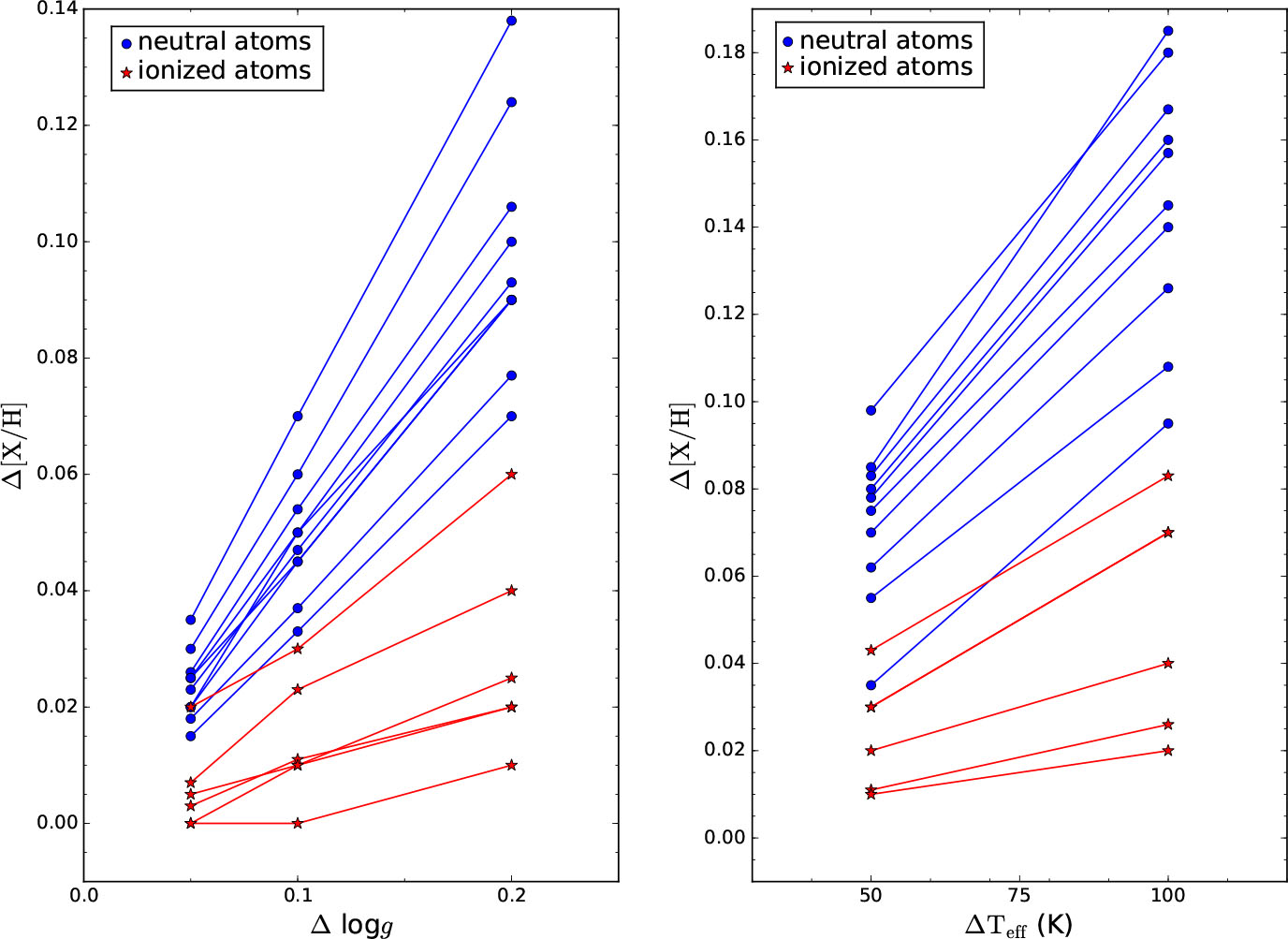
Fig. 6 Abundance discrepancy caused by log g (left panel) and Teff (right panel) variation for all the species.
Download figure:
Standard image3.3. Comparison with αCM
As we introduced in Section 2.3, we calculated two types of mixing-length parameter α models, one from the most commonly used BV theory and the other from the improved CM theory. The values for Δ[X/H]αBV and Δ[X/H]αCM are listed in Table 5 for comparison. Abundance discrepancies between two α models for each line were also calculated, as defined by,

The largest Δ [X/H]α = 2 is the specific line Sii 4102 Å which is up to 0.07 dex; some discrepancies are at a level of 0.05 dex. This discrepancy reflects the difference between the two α models with α = 2 and is expected because the α values in the two theories stand for the different efficiencies of convective energy transport. As Wu et al. (2015) suggested, α = 1 in CM theory best represents HD 122563, and we additionally calculated Δ [X/H] between αCM = 1 and αBV = 2. The recalculated Δ [X/H] did not exceed 0.04 dex. The real difference between two recalibrated α is modest.
The largest abundance discrepancy by αCM variation is 0.05 dex. Most Δ[X/H]αCM are smaller than 0.04 dex, which is consistent with Δ[X/H]αBV. Despite the slight difference between the BV and CM theory parameterization of the mixing-length parameter, the influence of the two α values on abundance determination is similar for HD 122563.
4. Conclusions
In this work, we studied how the mixing-length parameter α influences the abundance determination for several elements in the metal-poor giant HD 122563. The high-quality HARPS spectra of HD 122563 enabled us to determine the abundance discrepancy of 59 metallic lines in 16 species. We calculated a grid of 20 stellar models with different mixing-length parameters α, effective temperatures Teff and surface gravities log g, in steps of 0.5 dex, 50/100 K and 0.05/0.1/0.2 dex, respectively. We adopted a spectral synthesis method to derive the abundance for each metallic line. The abundance discrepancy between the grid models (Groups 1-5) and benchmark model (Group 0) was derived through a line-by-line differential method, and such an approach largely counteracted the uncertainty introduced by atomic data.
Overall, the influence of mixing-length parameter α is smaller than measurement uncertainty for the abundance determination in the metal-poor giant HD 122563. The largest Δ [X/H] caused by α variation is 0.05 dex. Mostly, Δ [X/H] is less than 0.03 dex. The average abundance discrepancy of all the elements is about 0.02 dex. The abundance discrepancies of the 16 species in HD 122563 are in line with our previous study of iron abundance (Song et al. 2020). The uncertainties introduced by convection mixing-length parameter α are lower than typical uncertainties in abundance determination for metal-poor stars. Even though α variation can cause a slight change in the shape of strong lines, we find no correlation between the abundance discrepancy and the line strength based on our study of HD 122563. The dependency of excitation potential and abundance on the mixing-length parameter α is insignificant in our analysis. There is also no obvious difference in abundance discrepancy between the neutral lines and ionized lines.
We have found that the convection results in a different influence on the shape of the weak and strong lines. This is expected as the wings and core of weak lines form in deeper layers, where the convection affects the wings and core similarly. However, in the case of strong lines, the core forms in a layer shallower than those that form the wings, so the convection influences the wings and core of the strong lines differently.
Besides the mixing-length parameter, we also investigate the influence of effective temperature and surface gravity on abundance determination for all the metallic lines we selected. By changing log g by 0.2 dex or Teff by 100 K, abundances obtained from strong lines change by 0.1 dex or more. Even with a small variation of Teff = 50 K, the average change in abundance of all metallic lines still exceeds 0.05 dex. Overall, the abundance discrepancy caused by Teff and log g variations is higher than the influence of convection. Therefore, the errors in Teff and log g introduce larger uncertainty on abundance determination than the convection mixing-length parameter α.
Moreover, we also compare the abundance difference derived from two different mixing-length parameters, one is based on BV theory and the other is based on CM theory. The abundance discrepancy due to αCM does not exceed 0.04 dex. Both mixing-length parameters show rather modest influence on abundance determination and minuscule deviation between each other.
Based on our analysis, convection can be safely ignored in most cases related with the abundance determination of metal-poor giants such as HD 122563. For 1D stellar atmospheric analysis, the accuracy of abundance determination does not strongly depend on the choice of the mixing-length parameter α, but the uncertainties in effective temperature and surface gravity play a more important role. On the basis of the neutral and ionized atomic lines we analyzed in this paper, we plan to study the influence of the convection mixing-length parameter on molecular bands in our future work.
Acknowledgements
We thank the anonymous referee for valuable suggestions and comments. This work was supported by the National Natural Science Foundation of China (Grant Nos. 11988101, 11890694, 11773033) and the National Key R&D Program of China (No. 2019YFA0405502). We thank Liang Wang for many helpful discussions. N. Song thanks K. F. Tan for his guidance in using SIU. This work is based on data products from observations made with the ESO Telescopes at the La Silla Paranal Observatory under programme ID 080.D-0347 (A).