Barycentric Corrections for Precise Radial Velocity Measurements of Sunlight

In extremely precise radial velocity (EPRV) work, the Sun is our only touchstone. We know its center-of-mass motion with respect to our observatories essentially perfectly, and we can resolve the surface spatially and spectrally with exquisite precision.

We can also determine the amount of variation the Sun should exhibit at any given moment by integrating disk-integrated Dopplergrams of a single spectral line to synthesize the sorts of observations we would make with our spectrographs, thus connecting the variability we observe in our spectrographs to physical phenomena on the Sun we understand. We can also use numerical models of the Sun validated against observations of it to interpret EPRV measurements of it and other stars (e.g., Cegla et al. 2013, 2018). The Sun is thus the ultimate RV "standard star."

These observations of the Sun as a star have been used to great profit, teaching us much about the limitation of EPRV work on Sun-like stars. For instance, Milbourne et al. (2019) compared precise radial velocities with data from the Solar Dynamics Observatory and SORCE satellite to determine the degree to which surface magnetic activity was causing RV variations.

But observing the Sun as a star is generally challenging: it is too large and too bright to collect its disk-integrated light into EPRV spectrographs without dedicated hardware. Several instruments, including the HARPS, HARPS-N, and NEID spectrographs, make good use of small solar telescope feeds to make observations of the Sun during the day (e.g., Collier Cameron et al. 2019).

Observations of the Sun at night (McMillan et al. 1993; Molaro & Centurión 2011; Haywood et al. 2016) are an elegant solution to the problem: the surfaces of the Moon and asteroids are good diffusive reflectors, providing a bright source of disk-integrated sunlight that can be observed with the very telescopes and optical fibers we use to observe stars. When observed this way, these sources are also immune to the effects of differential extinction across the solar disk that infect observations with solar telescopes, and their albedos change sufficiently slowly with wavelength that their reflection spectra will not interfere with EPRV measurements.

Indeed, Haywood et al. (2016) used simultaneous observations of Vesta and the Sun via the Solar Dynamics Observatory to deduce the physical origins of EPRV "jitter" on the Sun and test the value of chromospheric activity indicators in correcting for it. Lanza et al. (2016) used radial velocity measurements of the Sun in reflection to characterize the effects of the 11 yr solar cycle on long-term EPRV measurements.

Precise Doppler work requires careful correction for the motion of the observatory in the form of a "barycentric correction." In coarse work with stars, this means subtracting the velocity of the telescope (due to the orbital and rotational motion of Earth) in the direction of the star from the measured velocity to get the star's velocity with respect to the solar system barycenter.

Thanks to precise solar system ephemerides from the Jet Propulsion Laboratory (JPL; Folkner et al. 2014), tracking of Earth's orientation in space by the International Earth Rotation Service, and precise observatory coordinates from the Global Positioning System, the velocity vector of any observatory through the solar system can be computed quickly and easily. Applying this information to transform measured redshifts into radial velocity measurements is not trivial, however. The various aspects of the problem—including interpretation of the JPL ephemeris, handling perspective effects toward target stars, defining the effective time of observation in the presence of atmospheric effects, accounting for relativistic effects, and quantifying the uncertainties in the calculations—have been solved by multiple authors to the precision required for EPRV work on stars (e.g., Lindegren & Dravins 2003; Wright & Eastman 2014; Kanodia & Wright 2018; Blackman et al. 2019; Feng et al. 2019; Tronsgaard et al. 2019; Wright 2019).

However, one cannot simply enter the Sun's sky coordinates into a typical barycentric correction routine of the sort used by stellar astronomers and receive an easily interpreted result for a few reasons. Indeed, the concept of a "barycentric correction" for the Sun is not as clean or straightforward as the analogous concept for a star.

One complication is that the radial direction to the Sun is highly variable, and so many of the approximations used in such a barycentric correction routine are invalid. For instance, with other stars, the radial direction is approximately constant and changes in perspective cause small changes to the radial direction that can be treated as linear perturbations. For the Sun, the parallax is effectively π radians, not a fraction of an arcsecond, and so the "radial" direction is not even approximately constant. If one were to pick a constant "radial" vector for the Sun (say, the Sun's direction at the time of the first observation in a time series), then 3 months later one's measurements would contain almost no information about that component of the Sun's motion at all!

Another complication is that the purpose of making a barycentric correction is different for the Sun than for stars, so a proper philosophy of the calculation is unclear (see Section 3.2 of Wright & Eastman 2014). Here we are concerned with measuring the Sun's motion in the context of planet detection, in which case it is useful to imagine detecting, say, Jupiter via its gravitational influence on the Sun. But upon more careful consideration, it is not obvious what this means precisely.

In a stellar context, it means comparing two models: one in which a star has the planet in question and one in which it does not. For the first planet discovered orbiting a single star, this means comparing the null hypothesis of a star moving with constant velocity through space to one in which it is orbited by a single planet. In this case, the barycentric correction procedure is clear, because for the small perturbations caused by a planet, the problems of calculating Earth's motion and the star's motion due to a planet are separable.

In the case of the solar system, we know the Sun is orbited by planets, so strictly speaking we are dealing with a counterfactual, not a null hypothesis. But what is that counterfactual, exactly? Jupiter and the other planets accelerate Earth and our telescopes as much as or more than they accelerate the Sun. Is that counterfactual that the other planets do not exist, so Earth is a test particle on an unperturbed Keplerian orbit? Is it that Earth's motion is influenced by them, but the Sun is not? When we write that the Sun is not influenced by them, do we only mean that we pretend that the Sun's Doppler shift is zero in the frame of the solar system barycenter or that it also sits at the barycenter of the solar system? If the latter, how do we define the "radial" direction—from the observatory toward the apparent position of the solar disk center or toward the solar system barycenter? And so on.

We will see, however, that we can define a "barycentric correction" in the sense of the correction we must apply to a measurement to get the redshift we would measure in the barycentric frame in the direction of the object that sunlight illuminates. This is not a "radial velocity" as measured along a constant direction, but from the constantly (and nonuniformly) varying direction from Earth or other solar system object to the apparent Sun. The effects of the planets will thus not be that of true Keplerian orbital curves, and their effects on the Sun will not be concentrated at a single frequency and its harmonics.

It is perhaps conceptually simpler and more useful, then, to approach the problem with a better-defined question: what is the Doppler shift one should measure from a given observatory of a source of known frequency at the surface of the Sun? This can be computed using much of the machinery of a barycentric correction—a solar system ephemeris, Earth rotation parameters, accounting for relativistic effects—along with a few extra features unique to the problem (accounting for the finite speed of light and computing the retarded values of the position and velocity of the solar system objects used in reflection). Any variations from this expected value can then be attributed to other complexities of the problem such as the finite size of the Sun, stellar jitter, or instrumental effects.

While this problem has been solved by multiple groups, there has not previously been a publication that describes a standard method or analyzes the precision possible for such work with existing ephemerides. In this article, we explicate a rigorous barycentric correction algorithm for precise Doppler observations of sunlight and describe the public code that performs it. In Section 2, we describe the theory of calculating Doppler shifts from ephemerides, and in Section 3, we apply that theory to sunlight measured directly and in reflection. Section 4 describes our public code implementation, and Section 5 describes how uncertainties propagate from the JPL ephemerides to the barycentric correction. In Section 6, we use our code to simulate "perfect" observations of the Sun to assess the difficulty of "detecting" the solar system planets in such data.

The term "barycentric correction" is sometimes also used in the context of defining when an observation has taken place, to refer to the reduction of the local time of observation to the time when the starlight of the observation passed the solar system barycenter (SSB). Observations of the Sun should instead be reduced to the time the light was emitted from the Sun, defined below as t_e (see Section 3.2).

In this article, we follow the notation of Wright & Eastman (2014). All positions, velocities, and times are measured in the frame of the SSB. We make use of the JPL Horizons interface (Giorgini et al. 1997), which makes use of the DE series of ephemerides (Folkner et al. 2014).

The simplest case is observing the Sun directly. We begin simply, considering a single point on the surface of the Sun, so we can use Equations (1) and (3) of Wright & Eastman (2014):

$$\begin{eqnarray}&&z\equiv \displaystyle \frac{{\nu }_{\mathrm{emit}}-{\nu }_{\mathrm{meas}}}{{\nu }_{\mathrm{meas}}}\end{eqnarray} \tag{ 1 }$$

$$\begin{eqnarray}&&{\nu }_{\mathrm{meas}}={\nu }_{\mathrm{emit}}\left(\displaystyle \frac{(1+{z}_{\mathrm{GR},\odot })}{{\gamma }_{\odot }(1+{{\boldsymbol{\beta }}}_{\odot }\cdot {\hat{\rho }}_{\odot ,\oplus })}\right)\left(\displaystyle \frac{{\gamma }_{\oplus }(1+{{\boldsymbol{\beta }}}_{\oplus }\cdot {\hat{\rho }}_{\odot ,\oplus })}{(1+{z}_{\mathrm{GR},\oplus })}\right),\end{eqnarray} \tag{ 2 }$$

where the ⊕ symbol stands for the observatory and ⊙ for the Sun, and ${z}_{\mathrm{GR}}$ is the gravitational redshift from infinity to the observatory or solar surface.¹ Heuristically, the first term in parentheses in Equation (2) shifts the frequency of light from the Sun's rest frame into that of the SSB (at infinity), and the second shifts it from the frame of the SSB into that of the observatory.² Because of the light travel time in the system, we need to define when we are measuring these quantities. Specifically, let t be the time of observation and t_e be the time the photons were emitted. Then we have

$$\begin{eqnarray}&&{{\boldsymbol{\beta }}}_{\oplus }\equiv {{\boldsymbol{v}}}_{\oplus }(t)/c,\end{eqnarray} \tag{ 3 }$$

$$\begin{eqnarray}&&{{\boldsymbol{\beta }}}_{\odot }\equiv {{\boldsymbol{v}}}_{\odot }({t}_{e})/c,\end{eqnarray} \tag{ 4 }$$

$$\begin{eqnarray}&&{{\boldsymbol{\rho }}}_{\odot ,\oplus }\equiv {{\boldsymbol{r}}}_{\odot }({t}_{e})-{r}_{\oplus }(t),\end{eqnarray} \tag{ 5 }$$

$$\begin{eqnarray}&&\rho \equiv | {\boldsymbol{\rho }}| ,\end{eqnarray} \tag{ 6 }$$

$$\begin{eqnarray}&&\hat{\rho }\equiv {\boldsymbol{\rho }}/\rho ,\end{eqnarray} \tag{ 7 }$$

$$\begin{eqnarray}&&{z}_{{GR},\odot }=-\displaystyle \frac{{{GM}}_{\odot }}{{c}^{2}{R}_{\odot }},\end{eqnarray} \tag{ 8 }$$

$$\begin{eqnarray}&&{z}_{{GR},\oplus }=-\displaystyle \frac{{{GM}}_{\odot }}{{c}^{2}{\rho }_{\odot ,\oplus }}-\displaystyle \frac{{{GM}}_{\oplus }}{{c}^{2}{R}_{\oplus }},\end{eqnarray} \tag{ 9 }$$

where ${\boldsymbol{r}}$ and ${\boldsymbol{v}}$ refer to the position and velocity of an object, respectively, with respect to the SSB at some time.³ γ is the usual Lorentz factor computed from the corresponding β:

$$\begin{eqnarray}&&\gamma \equiv \displaystyle \frac{1}{\sqrt{1-{\beta }^{2}}},\end{eqnarray} \tag{ 10 }$$

We measure the redshift of the spectral features of sunlight with respect to some fiducial set of frequencies $\nu ^{\prime}$ that depend on the details of the measurement technique. We thus measure

$$\begin{eqnarray}&&{z}_{\mathrm{meas}}=\displaystyle \frac{\nu ^{\prime} -{\nu }_{\mathrm{meas}}}{{\nu }_{\mathrm{meas}}}\end{eqnarray} \tag{ 11 }$$

$$\begin{eqnarray}&&=\displaystyle \frac{\nu ^{\prime} }{{\nu }_{\mathrm{emit}}}\displaystyle \frac{(1+{z}_{\mathrm{GR},\oplus }){\gamma }_{\odot }(1+{{\boldsymbol{\beta }}}_{\odot }\cdot {\hat{\rho }}_{\odot ,\oplus })}{(1+{z}_{\mathrm{GR},\odot }){\gamma }_{\oplus }(1+{{\boldsymbol{\beta }}}_{\oplus }\cdot {\hat{\rho }}_{\odot ,\oplus })}-1\end{eqnarray} \tag{ 12 }$$

from our source.

Here we encounter a few other differences with the usual barycentric correction. We see that the scale factor $\nu ^{\prime} /{\nu }_{\mathrm{meas}}$ matters because we are interested in the direct connection between measured redshift and the precise, absolute motion of the Sun. (In exoplanet work, this factor is degenerate with the imprecisely known gravitational redshift, convective blueshift, and space motion of the star).

Now we can, following the notation of Wright & Eastman (2014), define

$$\begin{eqnarray}&&{z}_{\mathrm{true}}=\displaystyle \frac{\nu ^{\prime} }{{\nu }_{\mathrm{emit}}}\displaystyle \frac{{\gamma }_{\odot }(1+{{\boldsymbol{\beta }}}_{\odot }\cdot {\hat{\rho }}_{\odot ,\oplus })}{(1+{z}_{\mathrm{GR},\odot })}-1,\end{eqnarray} \tag{ 13 }$$

which captures all of the information about the redshift of the light of the Sun in its apparent direction as it would be observed from infinity, including the mean convective blueshift (captured in the $\nu ^{\prime} /{\nu }_{\mathrm{emit}}$ term) and the gravitational redshift. This last term produces a ∼634 m s⁻¹ offset from zero for all measurements compared to typical values observed at Earth.⁴

Then we can define a "barycentric correction" z_B that transforms our measured redshifts to this value

$$\begin{eqnarray}&&{z}_{{\rm{B}}}=\displaystyle \frac{{\gamma }_{\oplus }(1+{{\boldsymbol{\beta }}}_{\oplus }\cdot {\hat{\rho }}_{\odot ,\oplus })}{(1+{{\rm{z}}}_{{\rm{GR}},\oplus })}-1\end{eqnarray} \tag{ 14 }$$

such that, following Equation (10) of Wright & Eastman (2014),

$$\begin{eqnarray}&&(1+{z}_{{\rm{true}}})=(1+{z}_{{\rm{meas}}})(1+{z}_{{\rm{B}}}).\end{eqnarray} \tag{ 15 }$$

One thus has two paths to "correcting" one's measurements of the Doppler shift of the Sun (${z}_{\mathrm{meas}}$) for barycentric motions. The first is to model one's data using Equation (12), in which case the residuals will be due to measurement uncertainties, instrumental effects, and solar atmospheric effects (i.e., stellar jitter).

If, instead, one wishes to remove the effects of Earth's motion but retain the solar motion due to the planets, one can calculate z_B using Equation (14) and transform the measured redshifts to ${z}_{\mathrm{true}}$ using Equation (15). This should reveal, for instance, the ∼10 m s⁻¹ signal of Jupiter at its synodic period with Earth of 1.09 yr.

The $\nu ^{\prime} /{\nu }_{\mathrm{emit}}$ term cannot be computed from an ephemeris and depends on the details of the measurement technique and the motions in the solar atmosphere. In EPRV work, the templates or masks used to measure Doppler motions are usually chosen to keep this quantity as close to 1 as possible by setting the wavelengths of spectral features to those observed in sunlight. This means that for sunlight, the ratio will differ from 1 by no more than the radial velocity of an observatory toward the Sun in terms of the speed of light, which is of order 10⁻⁶. For computational purposes, we therefore set it to 1, which will result in a small, constant, multiplicative offset between the predicted and measured differential in redshifts. It will also produce errors in the barycentric-corrected velocities via cross-terms with ${\beta }_{\odot }$, which has an amplitude of 4 × 10⁻⁸ due to Jupiter. These cross-terms therefore have magnitude 4 × 10⁻¹⁴, corresponding to barycentric correction errors of the order of 20 μ s⁻¹.

It is not strictly necessary to consider the retarded position of the Sun here. The error in the computed Doppler shift from ignoring the finite speed of light scales⁵ as ${v}_{\oplus }{v}_{\odot }/c$. Because the Sun moves at only ∼10 m s⁻¹, only at work below 1 cm s⁻¹ would such effects begin to matter (retarded times will be important for other solar system objects, though).

The real Sun has finite size and so is not observed at (the retarded position of) its center of mass but at a range of angles and distances across its near hemisphere. This has important consequences when considering the effects of, say, differential atmospheric extinction across the disk, which will preferentially favor photons from one limb of the Sun, with its characteristic rotational velocity and barycentric correction.

The largest (first-order) effect of the varying barycentric correction comes from the tangential orbital motion of Earth, whose projection in the direction of the Sun is in the form of a gradient across the disk with amplitude 150 m s⁻¹, which is one order of magnitude smaller than the gradient due to solar rotation. Like solar rotation, the average of this correction across the disk, ignoring surface features and atmospheric extinction, is zero, so this effect need not be part of our calculation. The second-order effect is the decrease in the radial component of the velocity of the observatory toward the Sun as one observes away from disk center. This term does not average out but is smaller by a factor of 10⁴, so matters perhaps only at or below the 1 cm s⁻¹ level.

Solar system objects are essentially moving mirrors. We must calculate the Doppler shift they impose on light at the time the light strikes them. This requires knowing the location and velocity of the light at the time it was emitted, the location and velocity of the surface it strikes at the time it strikes it, and the location and velocity of the primary mirror of the telescope at the time the light arrives there.

Let t_m be the time that the sunlight strikes the surface of a solar system object, located at position ${{\boldsymbol{r}}}_{m}$. The object moving at speed ${{\boldsymbol{\beta }}}_{m}$ sees the Sun in direction ${\hat{\rho }}_{\odot ,m}$ as it was at time t_e, and at time t the observatory sees the solar system object in direction ${\hat{\rho }}_{m,\oplus }$ as it was at time t_m, where

$$\begin{eqnarray}&&{{\boldsymbol{\beta }}}_{m}\equiv {{\boldsymbol{v}}}_{m}({t}_{m})/c,\end{eqnarray} \tag{ 16 }$$

$$\begin{eqnarray}&&{{\boldsymbol{\rho }}}_{\odot ,m}\equiv {{\boldsymbol{r}}}_{\odot }({t}_{e})-{{\boldsymbol{r}}}_{m}({t}_{m}),\end{eqnarray} \tag{ 17 }$$

$$\begin{eqnarray}&&{{\boldsymbol{\rho }}}_{m,\oplus }\equiv {{\boldsymbol{r}}}_{m}({t}_{m})-{{\boldsymbol{r}}}_{\oplus }(t).\end{eqnarray} \tag{ 18 }$$

For an observer on the solar system object, we can calculate the observed frequencies of sunlight from Equation (2):

$$\begin{eqnarray}&&{\nu }_{\mathrm{meas},m}={\nu }_{\mathrm{emit}}\left(\displaystyle \frac{(1+{z}_{\mathrm{GR},\odot })}{{\gamma }_{\odot }(1+{{\boldsymbol{\beta }}}_{\odot }\cdot {\hat{\rho }}_{\odot ,m})}\right)\left(\displaystyle \frac{{\gamma }_{m}(1+{{\boldsymbol{\beta }}}_{m}\cdot {\hat{\rho }}_{\odot ,m})}{(1+{z}_{\mathrm{GR},m})}\right),\end{eqnarray} \tag{ 19 }$$

and similarly for an observer on Earth of that solar system object, we have

$$\begin{eqnarray}&&{\nu }_{\mathrm{meas}}={\nu }_{\mathrm{emit},m}\left(\displaystyle \frac{(1+{z}_{\mathrm{GR},m})}{{\gamma }_{m}(1+{{\boldsymbol{\beta }}}_{m}\cdot {\hat{\rho }}_{m,\oplus })}\right)\left(\displaystyle \frac{{\gamma }_{\oplus }(1+{{\boldsymbol{\beta }}}_{\oplus }\cdot {\hat{\rho }}_{m,\oplus })}{(1+{z}_{\mathrm{GR},\oplus })}\right).\end{eqnarray} \tag{ 20 }$$

Because the Doppler shift imparted by the solar system object in its own frame is zero, we have ${\nu }_{\mathrm{meas},m}={\nu }_{\mathrm{emit},m}$. Then, the redshifts observed at Earth are

$$\begin{eqnarray}&&\begin{array}{l}{z}_{\mathrm{meas}}=\displaystyle \frac{\nu ^{\prime} }{{\nu }_{\mathrm{emit}}}\\ \times \,\left[\displaystyle \frac{(1+{z}_{\mathrm{GR},\oplus }){\gamma }_{\odot }(1+{{\boldsymbol{\beta }}}_{\odot }\cdot {\hat{\rho }}_{\odot ,m})(1+{{\boldsymbol{\beta }}}_{m}\cdot {\hat{\rho }}_{m,\oplus })}{(1+{z}_{\mathrm{GR},\odot }){\gamma }_{\oplus }(1+{{\boldsymbol{\beta }}}_{m}\cdot {\hat{\rho }}_{\odot ,m})(1+{{\boldsymbol{\beta }}}_{\oplus }\cdot {\hat{\rho }}_{m,\oplus })}\right]-1.\end{array}\end{eqnarray} \tag{ 21 }$$

The "barycentric correction" in this case is

$$\begin{eqnarray}&&{z}_{{\rm{B}}}=\displaystyle \frac{{\gamma }_{\oplus }(1+{{\boldsymbol{\beta }}}_{\oplus }\cdot {\hat{\rho }}_{{\rm{m}},\oplus })}{(1+{{\rm{z}}}_{{\rm{GR}},\oplus })}\displaystyle \frac{(1+{{\boldsymbol{\beta }}}_{{\rm{m}}}\cdot {\hat{\rho }}_{\odot ,{\rm{m}}})}{(1+{{\boldsymbol{\beta }}}_{{\rm{m}}}\cdot {\hat{\rho }}_{{\rm{m}},\oplus })}-1.\end{eqnarray} \tag{ 22 }$$

Note that this corrects measurements to the vantage of the solar system object, not Earth. That is, the dominant signal in the barycentric-corrected velocities of Ceres will be the Sun's motion due to Jupiter in the direction of Ceres, modulated at their synodic period.

For reflected light observations, we need to take into account the light travel time. One can do this iteratively to estimate the position and velocity of the reflected light observation target until the calculated Doppler shift converges. In our code implementation (Section 4), we obtain the light travel time directly from our Horizons call for the solar system object, where we first query for the position of the solar system object with respect to the observatory at the time of exposure (t), which also gives us the light travel time. We use this light travel time to calculate the retarded position of the target (t_m), and then perform a similar step to calculate the light travel time from the solar system object and the Sun, to obtain the time of emission (t_e) from the Sun.

Fortunately, solar system objects act as good diffuse reflectors and so provide disk-integrated sunlight much the same way telescopes collect disk-integrated starlight. There are some drawbacks to observing them, however.

Unlike with the Sun, using the retarded position of the solar system object may be important. The Doppler shift error from ignoring this term is of order ${v}_{1}{v}_{2}/c$, where both velocities in this case are of order 20 km s⁻¹, implying typical errors of order ∼1 m s⁻¹. These light travel times thus need only be precise to 1 part in 100 or so for 1 cm s⁻¹ precision, so approximating light travel times using the instantaneous positions of the bodies at the time of observation is sufficient.

Also unlike the Sun, objects such as Ceres, Vesta, and Pallas can have highly variable surface brightness and phases, which cause asymmetric rotational broadening (Lanza & Molaro 2015; Haywood et al. 2016; Molaro et al. 2016). Because they are not point sources, they fill the telescope pupil differently from stars and so are not perfect proxies for the Sun as a star (Molaro et al. 2008). Also, observing at true opposition can create unexpected effects (Molaro et al. 2015).

Inelastic scattering may also be a concern. Observations of planetary atmospheres can suffer from the the Ring effect (Grainger & Ring 1962), caused by Raman, Brillouin, and other forms of scattering. To first order, the effect is to "fill in" the lines of the solar spectrum (Pallamraju et al. 2000), but a wavelength shift is also present (Cochran et al. 1981). This effect (to say nothing of wind) complicates attempts to measure the Doppler velocity of the Sun using blue sky measurements (Gray et al. 2000; Molaro et al. 2008). We are not aware of a documented case of a similar effect from planetary surfaces, but if one is present, it would be a function of scattering angle and so present additional complexities.

Wright & Eastman (2014) considered the Shapiro delay, caused by the general relativistic distortion of spacetime as starlight passes by the Sun or Jupiter, because its time derivative (due to the motions of the observer and the source of the delay) introduces a small Doppler shift. For stars within tens of degrees of the Sun, the effect can matter at the mm s⁻¹ level, and for relatively bright solar system objects even closer to the Sun, it may matter even more. The effect is even smaller for Jupiter, even when stars are within ${1}^{{\prime} }$ of it, but the Galilean satellites can approach even closer than that.

We have not included this effect in our calculations or in barycorrpy because it is small and application of Equation (23) of Wright & Eastman (2014) to correct for it is nontrivial: the effect depends not only on the angular separation between the Sun (or Jupiter) and the reflecting body, but on their orientation (it should be relevant only when the reflecting object is behind the Sun or Jupiter), and needs to be considered for both legs of the journey to Earth. Work near or below cm s⁻¹ precision may need to include a small correction for sources near the Sun or Jupiter.

Using our code, we have simulated observations of the Sun every 10 days from the Cerro Tololo Inter-American Observatory for 30 yr to explore how well the effects of the solar system planets can be inferred from solar RVs (as ${z}_{\mathrm{predicted}}$, above). We chose this uniform cadence because it is much faster than any relevant frequencies in the problem and so will not generate any aliased power in our periodograms.

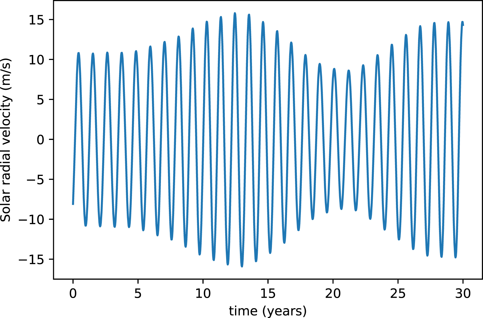
Applying the barycentric correction formalism above to determine ${z}_{\mathrm{true}}$ for these observations, we can isolate only the motion of the Sun in the direction of the observatory, having removed all Doppler components of the observatory motion from the signal. Figure 1 shows this result, which has a strong signal at the synodic period of Jupiter with amplitude of ∼10 m s⁻¹.

Zoom In Zoom Out Reset image size

This is not surprising, as Jupiter is responsible for most of the Sun's motion, and we observe an ever-changing perspective on that motion at that synodic period.

Because our synthetic data are noise free and periodically sampled, we can take a Fourier transform to determine the ideal periodogram one could achieve in 30 yr of daily observations.

We present the result in Figure 2. The 12 m s⁻¹ "wobble" of the Sun due to Jupiter is seen to be broadly distributed across a range of frequencies with a peak at the synodic period of Jupiter. The width of this signal is likely due to the combination of the significant eccentricity of Jupiter (e = 0.049) and the noncommensal periods of Jupiter and Earth, which conspire to generate a nonperiodic RV signal. That is, in the barycentric frame corotating with Earth, Jupiter's orbit is neither circular nor periodic, and so does not produce power at a single frequency and its harmonics.

Zoom In Zoom Out Reset image size

The wide wings of this power extends well into the synodic periods of the other planets. There is no peak at the synodic period of Venus, the next most significant planet in the time series, presumably because it is buried beneath the broad signal of Jupiter.

It is therefore quite challenging to "detect" the presence of any planet other than Jupiter (and possibly Saturn) even with perfect, daily measurements of the Sun for 30 yr. One would need to first subtract the signal of Jupiter to recover that of Venus, the next strongest signal, but this is not straightforward and requires carefully choosing a counterfactual of the sort discussed in Section 1.2.

For instance, one might construct an artificial ephemeris by using the true positions of Jupiter and the Sun from the JPL ephemeris, but ascribing to the Sun velocities calculated from accelerations due only to Jupiter. Because the indirect effects of Venus on the positions of Jupiter and the Sun are small, this is likely a sufficiently precise ephemeris to feed barycorrpy in predictive mode such that the only remaining signal is the radial motion of the Sun due to the planets other than Jupiter. The signal of Venus could then be similarly calculated and searched for in the residuals via a matched filter or in a manner analogous to exoplanet hunting via model fitting, perhaps with Bayesian and MCMC methods.

To use solar RV measurements to prove the precision of an RV spectrograph to terrestrial, habitable-zone planets, it would be simpler, perhaps, to subtract the known signal of all of the planets and perform an injection-recovery test to see if one would be sensitive to Venus if one observed the Sun from a fixed vantage.

We have also computed the radial velocities one would measure in reflection from Ceres at the same times. Because our purposes here are purely illustrative, we have calculated these velocities every 10 days for 30 yr without regard to the true observability of Ceres or to the complexities described in Section 3.3 (e.g., Molaro et al. 2015). The raw radial velocities are dominated by the diurnal motion of Earth, but the barycentric-corrected velocities show structure at many long frequencies (Figure 3). The signal of Jupiter is clearly visible, but there is also significant power at other frequencies, likely due to the significant eccentricity in the orbit of Ceres.

Zoom In Zoom Out Reset image size

Because the synodic period between Jupiter and Ceres is so long (Ceres has an orbital period of 4.6 yr), even after 30 yr there is very little frequency resolution in the resulting Fourier transform, shown in Figure 4, making it difficult to determine whether the signal of Saturn is present.

Zoom In Zoom Out Reset image size

Interestingly, the synodic periods of Earth and Venus in these data sets are sufficiently distinct from that of Jupiter that their signals clearly stand out in these noiseless data, as seen in Figure 4. They are not sharply peaked, however, presumably due to the orbital eccentricity of Ceres. This suggests that if the difficulties in making precise radial velocity measurements of Ceres (or other asteroids) can be overcome, that a sufficiently dense and long time series of them might be a good proxy for detecting habitable-zone terrestrial planets.