
Abstract
Originated in 1991 by O'Regan and Grätzel, dye-sensitized solar cells (DSSCs) provide alternative solutions for renewable energy problems. Earlier mathematical models for DSSCs are based on junction solar cells, which was first studied by Chapin et al in 1954. These equations were derived from Shockley's work on modelling semiconductors in the late 1940s. However, it was pointed out by Cao et al and Gregg that diffusion model is more suitable for modelling DSSCs. Since the study by Södergren in 1994, the diffusion model has become prevalent in literature and the development of this model by including additional equations to incorporate electrolyte concentrations, time dependence for charge carrier densities and nonlinear diffusivity has shown to capture more complex processes of charge transport within DSSCs. In this paper, we review the development of the diffusion model for the charge carrier densities in a conduction band of DSSCs.
Export citation and abstract BibTeX RIS

Original content from this work may be used under the terms of the Creative Commons Attribution 4.0 licence. Any further distribution of this work must maintain attribution to the author(s) and the title of the work, journal citation and DOI.
This article was updated on 22 April 2021 to add permission lines to the figures.
1. Introduction
The demand for renewable energy is greater than ever, with Earth's oil reserves expected to expire by the end of the century [1]. Though 85% of the world's energy demands are met by fossil fuels [2], the renewable energy sector is projected to fulfil 33% of the world's energy supplies by 2030 [3].
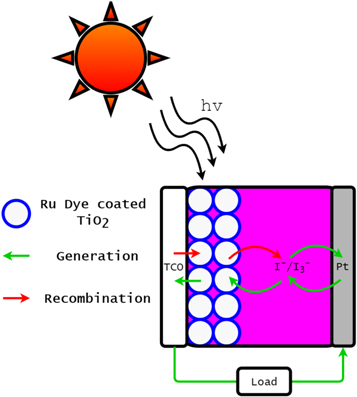
Since their inception in 1991, dye-sensitized solar cells (DSSCs) have proven a unique, low-cost approach to harvesting renewable energy [4]. Standard DSSCs comprise four fundamental components, namely photosensitive dye, nanoporous semiconductor, electrolyte couple and counter electrode. Figure 1 outlines the components of a DSSC together with their intended functionality (outlined in the following section). DSSCs offer flexibility in the selection of materials and the design of these components, creating an active niche of research.
Download figure:
Standard image High-resolution image1.1. Function of DSSCs
In essence, there are seven main chemical reactions used to describe DSSCs in operation [1, 6]. Four of these chemical reactions enhance the performance of DSSCs, whereas the other three mechanisms are detrimental to the generation of electricity.
In DSSCs, photosensitive dye molecules absorb photons and enter an excited energy state:

where S is the dye molecule, h is Planck's constant and ν is the frequency of the photon. The photosensitive dye is designed to use this excited energy state to donate (or inject) electrons into the semiconductor's conduction band:

The photosensitive dye is regenerated by the electrolyte couple:

where M is the electrolyte and Mox is the oxidized electrolyte. This process enables the chemical reaction (1) to repeat. Finally, regeneration of the electrolyte is carried out by the counter electrode:

As a result of chemical reactions (1) to (4), a DSSC is able to generate electricity provided that there is sufficient sunlight as an energy input. However, DSSCs are also subject to loss mechanisms, which generally involve recombination of electron at interfaces. Excited dye molecules do not necessarily inject electrons into the conduction band as described by chemical reaction (1), instead they may emit the photon as radiation:

Alternatively, injected electrons may recombine with the DSSC before leaving the device to power a load. Active electrons in the semiconductor's conduction band may be used for regeneration either in the dye or in the electrolyte, which are respectively described by


Construction of DSSCs must therefore enhance reactions (1) to (4) and reduce the potential loss of electrons through the processes (5) to (7).
1.2. Components of DSSCs
1.2.1. Photosensitive dyes
The unique feature of DSSCs is its photosensitive dyes which are used to absorb sunlight [6]. Even though several types of dye molecules have already been proposed, the development of new dyes continues an active area of research.
One of the dyes that saw continual use since its introduction is the Ruthenium(II) N3 dye [7, 8]. The relationship between the molar absorption coefficient of N3 dye and the wavelength is given in figure 2 [8]. In their paper, Wu et al [8] show that the molar absorption coefficients of CYC-B1 and CYC-B5 dyes are generally higher than that of N3 dye, despite their inferior performances at lower wavelengths. However, the Ruthenium based N3 dye has continued its popularity, owing to its broad light absorption spectrum, increased duration in the excited state and high thermal stability [9, 10].
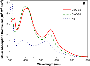
Figure 2. Relationship between molar absorption coefficient and wavelength (nm) for three commonly used dyes (N3, CYC-B1 and CYC-B5). Reprinted from [8], Copyright (2010), with permission from Elsevier.
Download figure:
Standard image High-resolution imageAnother well-known Ruthenium based dye is N719 [3]. The absorption coefficient of N719 relative to the wavelength is shown in figure 3 [11]. From the figure, we see that the absorbance of the N719 dye is greatly improved when anchored to the ZnO semiconductor as opposed to  .
.
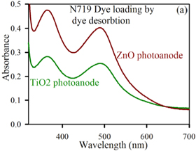
Figure 3. Plot of N719 absorbance against wavelength (nm). Reprinted from [11], Copyright (2019), with permission from Elsevier.
Download figure:
Standard image High-resolution image1.2.2. Nanoporous semiconductor
Given that the nanoporous semiconductor is responsible for the bulk of the electron transport in DSSCs, the choice of semiconductor is extremely important. A nanoporous semiconductor requires a wide band gap, which allows electrons to easily receive energy from excited dye molecules. In table 1, we summarise commonly used semiconductors together with their band gaps and efficiencies [12].
Table 1. Nanoporous semiconductors used in DSSCs [12].
| Semiconductor | Band Gap | Efficiency |
|---|---|---|

| 3.23 | 12.30% |
| ZnO | 3.30 | 5.60% |
| Nb2O5 | 3.49 | 5.00% |
| Zn2SnO4 | 3.70 | 3.70% |
| SrTiO3 | 3.20 | 1.80% |
| WO3 | 2.60–3.00 | 0.75% |
| SnO2 | 3.60 | 0.30% |
From table 1 we see that  vastly surpasses other semiconductors by way of efficiency. In their paper, Lau et al [12] show that
  is generally regarded as superior for its wide band gap, low cost and resistance to photo-corrosion. Figure 4 shows the porous structure of
  under electron microscope [13].
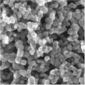
Figure 4. SEM image of the nanoporous  . Reprinted from [13], Copyright (2003), with permission from Elsevier.
Download figure:
Standard image High-resolution image1.2.3. Electrolyte couple
The electrolyte couple (sometimes referred to as the redox couple or charge mediator [6]) in the DSSC is designed to regenerate the photosensitive dye once it has been ionized by the process of electron injection (via reactions (1) and (3)). The iodide-triiodide redox couple  -
- is used almost universally [1, 14–18], since other electrolytes such as Br−-
 and SCN−-
 exhibit poor power conversion efficiencies compared to iodide-triiodide redox couple [19].
1.2.4. Counter electrode
Within a functioning DSSC, the counter electrode reintroduces electrons back to the DSSCs by allowing the electrolyte to replace the electrons lost in dye regeneration (as shown in reaction (4)) [6]. Counter electrodes are typically platinum (as seen in [12, 14, 15, 17, 18, 20–25]). Although known for its efficiency, major deterrents for using platinum as a counter electrode include its scarcity (increaseing production costs) [26] as well as its instability when it is used in conjunction with corrosive electrolyte couples [27].
In 2007, carbon nanomaterials were found to provide a unique and novel solution to both issues associated with the use of platinum counter electrodes [27–29]. In particular, Huang et al [28] investigate a DSSC with hard carbon spherule (HCS) as counter electrode. Though its efficiency of 5.7% is lower than the benchmark 6.5% of the DSSC with Platinum counter electrode, there are improvements in conductivity and resistance to corrosion.
1.3. Mathematical models
One approach to modelling DSSCs is based on the study of traditional junction solar cells. In particular, the drift-diffusion equations are used to describe the electron density in the semiconductor's conduction band while the hole density in the semiconductor's valence band and the strength of the electric field are modelled by Poisson's equation [2, 15, 30]. These equations are inherited from the models for the silicon solar cells pioneered by Chapin et al [31] and are based on Shockley's mathematical models for semiconductors [32]. Although this approach may benefit from the studies in the past decades, Gregg [33] mentions that it is not necessarily the best modelling approach for DSSCs. This is because the electric field is considered to have a negligible effect on the overall operation of DSSCs and is therefore ignored in subsequent models of DSSCs [22]. In this paper, we review the development of the diffusion models for DSSCs.
2. Diffusion model
The diffusion model is used to determine the electron density in the semiconductor's conduction band of a DSSC. Based on the electron density, other important parameters related to the performance of DSSCs can be obtained, including the short-circuit current density Jsc , the open-circuit voltage Voc and eventually the efficiency η.
2.1. Diffusion equations
Due to the structure of DSSCs, only one spatial dimension is considered. Given a DSSC of thickness d, we orient the device so that the counter electrode is located at x = d. From this, the conduction band electron density n(x, t) at position x and time t in the DSSC obeys the following partial differential equation (PDE) [34]:

where D(n) is the density-dependent diffusion coefficient, G is the spatially dependent electron generation term and R(n) is the density dependent recombination term. For DSSCs, we assume no electron flux at the counter electrode, giving rise to the boundary condition [35]

The electron density at the TCO interface (x = 0) is dependent on the bias voltage V on the DSSC [36], and is given by

where neq
is the dark equilibrium electron density, m is the ideality factor, q is the electron charge, kB
is Boltzmann's constant and T is the temperature of the DSSC. For short-circuit conditions, we set V = 0 and use the resulting boundary condition  . Under open-circuit conditions (J = 0), an alternative boundary condition for x = 0 is given by [37]

which allows us to compute the electron density if Voc is unknown. The DSSC is assumed to be initially at equilibrium, giving the simple initial condition

This model was developed in 1994 by Södergren et al [36], in which the steady-state special case was considered under the assumptions of linear diffusion and recombination with the boundary conditions based on short-circuit conditions (V = 0). This diffusion model is a popular choice for modelling DSSCs (as seen in [20, 36–39]). In particular, the linear diffusion equation is coupled with electrolyte equations in some models (which are discussed in more detail in section 2.5)
In 1996, Cao et al [22] extended this model to include time dependence, resulting in the first PDE for electron diffusion. This paper also suggested the first nonlinear version of the equation, with the diffusion coefficient D(n) = n.
2.2. Diffusion coefficient
The diffusion coefficient D(n) in equation (8) is an important component, as it reconciles the boundary condition  with the source term G(x) that is typically at its maximum at x = 0. In the diffusion model of Södergren et al [36], the diffusion coefficient is assumed to be a constant,

Though many papers adopt a constant value for D0 [35, 36, 40], a study in 2006 introduced a model incorporating the effect of the porosity of the nanoporous semiconductor into the diffusion coefficient [38].
In particular, Ni et al [38] gave the following expression for the diffusion coefficient that is dependent on the porosity p of the nanoporous semiconductor ( in this case):

2.3. Electron generation models
The electron generation term G(x) in (8) is a source term designed to incorporate the increase of conduction band electrons induced by sunlight exposure. The Beer–Lambert model is used exclusively, and is given by

where photons absorbed are in the wavelength range ![$[{\lambda }_{\min },{\lambda }_{\max }]$](https://content.cld.iop.org/journals/2399-6528/4/8/082001/revision7/jpcoabacd6ieqn14.gif) , ηinj
is the electron injection efficiency (the proportion of electrons successfully injected into the semiconductor conduction band, also referred to as Φinj
and ηinj
), ϕ is the wavelength dependent incident photon flux and α is the wavelength dependent absorption coefficient of the photosensitive dye.
, ηinj
is the electron injection efficiency (the proportion of electrons successfully injected into the semiconductor conduction band, also referred to as Φinj
and ηinj
), ϕ is the wavelength dependent incident photon flux and α is the wavelength dependent absorption coefficient of the photosensitive dye.
For ease of computation, several papers omit wavelength dependence in (14) (such as [22, 37, 41, 42]), leading to a simplified Beer–Lambert model of the form

where φ is an integrated version of ϕ and wavelength dependence of α is omitted. This generalized form of the Beer–Lambert law is also used in [43–45], for example.
We comment that equation (15) was first introduced by Södergren et al [36], who considered two simplified forms of (14). The first form, which is 15, assumes that substrate-electrode (SE) illumination is located at x = 0. The second form assumes that electrolyte-electrode (EE) illumination is located at x = d. In this case, the Beer–Lambert law is of the form [20, 46]

Finally, an analytical approach to model the electron generation term was developed by der Maur et al [16]. Their analytical model is motivated by relaxing the assumption of a constant absorption coefficient in DSSC modelling. By applying a rate equation to the density of photoactive dye molecules and a continuity equation on the electron generation term, their model for electron generation term, referred to here as g(x), is given implicitly by

where τr
is the dye regeneration time, σ is the attenuation cross section of the absorbing dye molecule and D0 is the total density of photoactive dye molecules. If τr
= 0, we recover the classical Beer–Lambert model  . This extended model allows the DSSC modelling to incorporate the effect of light intensity on electron generation within an operating DSSC.
2.3.1. Incident photon flux
Central to the Beer–Lambert equation (14) is the incident photon flux ϕ, which is the input from sunlight. Figure 5 is a plot of ϕ, the measured AM1.5 solar spectrum against wavelength λ [47].
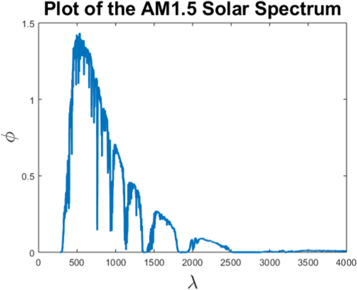
Figure 5. Plot of ϕ (Wm−2nm−1) against wavelength λ (nm) [47].
Download figure:
Standard image High-resolution imageThe literature models the input of sunlight in solar cells by two expressions, namely the incident photon flux and the sunlight intensity. Though equivalent, the incident photon flux considers the photons per unit area provided by sunlight, which has unit  . On the other hand, sunlight intensity is a measurement of the AM1.5 solar spectrum, which considers sunlight as energy per unit area, so that the unit is given by Wm−2. Dividing the sunlight intensity (Wm−2) by energy (Joules), we can convert from the sunlight intensity to photon flux (m−2s−1). Here, the energy we use is defined as the energy of a photon,

where h is Planck's constant, c is the speed of light and λ is the wavelength of the photon.
In the Beer–Lambert expression G(x), ϕ is usually considered as a photon flux and assumed to be a constant φ. The majority of the literature agrees upon φ = 1017 cm−2s−1 [37–39, 48, 49]. Nevertheless, other values used for φ include 1.5 × 10¹⁷ [1], 4.5 × 10¹⁵ [20], 9.87 × 10¹⁶ [41], 5 × 10¹⁶ [50] and 8.19 × 1016 cm−2s−1 [51].
Instead of assuming ϕ as a constant φ, we can use Planck's law, or an approximation to Planck's law to prescribe ϕ as a function of wavelength [52], namely

Integrating ϕ over all wavelengths, we have
where Γ is the gamma function defined by  and ζ is the Riemann zeta function, given in its integral definition by [53]
As Γ(4) = 3! = 6 and ζ(4) = π4/90 [54], we obtain

Under the standard temperature T = 5800 K, we have φ ≈ 6.4168 × 10⁷ Wm−2. This value justifies the assumption of a constant φ = 1017 cm−2s−1 as used in [37–39, 48, 49].
Alternatively, Anta et al [40] define the incident photon flux as

where ![$F\in [0,1]$](https://content.cld.iop.org/journals/2399-6528/4/8/082001/revision7/jpcoabacd6ieqn18.gif) is an irradiance coefficient used to measure the intensity of the sunlight. Integrating this form of ϕ over all wavelengths gives
is an irradiance coefficient used to measure the intensity of the sunlight. Integrating this form of ϕ over all wavelengths gives
Using F = 1 and T = 5960 K [40], we find φ ≈ 8.5237475580 × 1025m−2s−1.
Finally, Malyukov et al [55] propose the integral equation for ϕ as

where C is a coefficient used to model the atmosphere's influence on available photons for the DSSC, Rs is the radius of the Sun and r0 is the average distance from Earth to the Sun. The parameter F has the same meaning as in the model by Anta et al [40]. Integrating this expression over all possible wavelengths, we find
Though there is no analytical expression for ζ(3), the result is a finite number known as Apéry's constant [56]. With Rs = 6.9951 × 10³ m [57], r0 = 1.495978707 × 10¹¹ m [57] and F = 1, we have φ ≈ 4.8144702590 × 10¹¹m−2s−1.
The values of φ from the literature and from the above derivations are summarised in table 2 (given in units m−2s−1).
Table 2. Numerical values for the constant φ used in DSSC modelling (in m−2s−1).
| Value | Author | References |
|---|---|---|
| 9.87 × 10²⁰ | Lee et al 2004 | [41] |
| 1021 | Gómez and Salvador 2005 | [37] |
| 8.52 × 1025 | Anta et al 2006 | [40] |
| 4.5 × 10¹⁹ | Barnes et al 2009 | [20] |
| 1.5 × 10²¹ | Andrade et al 2011 | [1] |
| 5 × 10²⁰ | Bertoluzzi and Ma 2013 | [50] |
| 8.19 × 10²⁰ | Shi et al 2013 | [51] |
| 4.81 × 10¹¹ | Malyukov et al 2014 | [55] |
2.3.2. Absorption coefficient
The wavelength-dependent absorption coefficient α(λ) (sometimes referred to as αab to avoid ambiguity with other parameters with the same name) is usually assumed to be a constant, despite a clear relationship with wavelength as shown in figures 2 and 3.
Other model for α is given by Ni et al [38] where the absorption coefficient is assumed to be dependent on porosity p of the nanoporous semiconductor, namely

2.4. Recombination models
In contrast to the electron generation, electron recombination has seen a great variety of modelling approaches. The first such model is shown in Södergren et al [36] which is given by
where neq is the dark equilibrium density and τ0 is the electron lifetime. Referred to as the first order recombination [35, 36], this model is used frequently for its simplicity (used in [20, 37–39, 41, 46, 49, 55]).
Simple extension to this recombination term includes introducing nonlinear recombination rate (as considered in Fisher et al [58] and Barnes et al [48]):
where kR = 1/τ0 is a recombination constant and β is the order of recombination. In particular, Fisher et al [58] consider second order recombination (β = 2) and Barnes et al [48] consider 0 < β < 1.
A slight modification of this model is given in Anta et al [40] as
This recombination term is used in [40] in conjunction with the diffusion coefficient  . The extra factor (n − neq
) is introduced to facilitate the effectiveness of recombination based on the electron density and its relative distance from equilibrium.
. The extra factor (n − neq
) is introduced to facilitate the effectiveness of recombination based on the electron density and its relative distance from equilibrium.
Finally, in Nithyanandam et al [2] and Tanaka [59], a nonlinear recombination model is proposed to incorporate the role of the electrolytes in the DSSCs:
where the bar notation denotes the equilibrium values. This equation together with the model proposed by Nithyanandam et al [2] are not popularly used for DSSCs. This is because the model is based on a drift-diffusion equation, and since the effect of drift is negligible in DSSCs [22, 33], pure diffusion models are more widely adopted for DSSCs.
2.5. Electrolyte densities
The diffusion equation given by (8) is primarily concerned with the electron density in the conduction band. Here, we summarise the extended model of DSSCs that also include the effect of electrolyte concentrations. This model allows insights into the distribution of charged particles in DSSCs beyond the nanoporous semiconductor.
The earliest model in this area was published in 1996 by Papageorgiou et al [60]. Although this model does not consider the influence of electrons in the conduction band on the electrolytes, it provides the framework for such extension, which is investigated by Andrade et al [1]. In [1], the iodide-triiodide electrolyte couple is modelled by the following diffusion equations:


where  and
and  are the densities of the iodide and triiodide, respectively,
  and
and  are the diffusion coefficients of the iodide and triiodide and p is the porosity of
  . The accompanying initial and boundary conditions result from assuming a given initial concentration, a net flux of zero at the TCO electrode and a constant total concentration throughout the operation [1]. Mathematically, we can express these conditions as


where  and
and  are respectively the initial concentrations of the iodide and triiodide.
So far, this is the only model for the electrolyte couple under pure diffusion, and is used in a number of papers, such as [1, 25, 35, 55].
2.6. Current-voltage relationship
The purpose of modelling electron density by diffusion is to use the computed conduction band electron density to determine the current-voltage relationship in DSSCs. From there, we may calculate efficiency. Included with the diffusion model given by Södergren et al [36], the paper also provides the derivation of the J − V characteristics of a DSSC based on the diode equation.
The diode equation for current J as a function of voltage V is given by

where Jsc is the short-circuit current density, J0 is the reverse saturation coefficient, q is the electron charge, m is the ideality factor, kB is Boltzmann's constant and T is the temperature of the DSSC. By construction J(0) = Jsc . Likewise, we define the open-circuit voltage Voc to be the solution to J(Voc ) = 0.
We obtain the short-circuit current density Jsc and the open-circuit voltage Voc from the electron density n(x), which is the solution to the diffusion equation:

under the boundary conditions given in section 2.1. The photocurrent density J is given by [61]

where q is the electron charge. As the short-circuit current density Jsc is found by this equation under short-circuit conditions (in which the bias voltage V = 0 for the electron density nsc ), this yields the expression [35]

where  is the electron diffusion length. The open-circuit voltage is found by solving equation (8) under the alternative boundary condition
  to find the open-circuit electron density noc
. Therefore, the open-circuit voltage is found by
to find the open-circuit electron density noc
. Therefore, the open-circuit voltage is found by

Using the expressions for Jsc and Voc , we obtain the dark saturation current density as given by Södergren et al [36] as
2.7. Efficiency
The performance of DSSCs can be determined from the efficiency of the devices. The efficiency η is defined as [62]

where Pin is the total power available from sunlight. For the AM1.5 solar spectrum, Pin is taken to be 1000 Wm−2 [63]. We calculate power by the standard formula P = JV, which takes the form

To find the maximum power point  , we optimise P over V to obtain Vmax and then compute
  . Differentiating both sides of equation (36) with respect to V, we obtain
As all parameters in the expression for  are positive, we get
  for all voltages
 ![$V\in [0,{V}_{{oc}}]$](https://content.cld.iop.org/journals/2399-6528/4/8/082001/revision7/jpcoabacd6ieqn33.gif) . Thus, all critical points will be maximum values in this domain. Using the Lambert-W function, we obtain an explicit expression for the maximum power point, given by
. Thus, all critical points will be maximum values in this domain. Using the Lambert-W function, we obtain an explicit expression for the maximum power point, given by
Therefore, the maximum power output of the DSSC is given by
We compute the short-circuit current density Jsc and the open-circuit voltage Voc under each model by using the expressions given in equations (33) and (34). In section 4, we calculate efficiencies for DSSCs using these equations.
2.8. Incident photon to current efficiency
In addition to efficiency η, the incident photon to current efficiency (IPCE) curve can be used to gauge the performance of DSSCs with regard to photons of a particular wavelength. While it is used as a performance indicator, the short-circuit current density Jsc may be calculated using the IPCE(λ) by [6]

where h is Planck's constant, c is the speed of light, q is the electron charge and ϕ is the incident radiative flux. There are several definitions for IPCE(λ). The first definition is directly from O'Regan and Grätzel [4],
where LHE(λ) is the wavelength dependent light harvesting efficiency, ϕinj is the electron injection efficiency (also denoted by ηinj ) and ηe is the electron collection efficiency.
An alternative definition for IPCE  is given in Tanaka [59],

where Jsc is the short-circuit current density and ϕ is the incident radiative flux.
We note that the quantity hc/q is often replaced by the numerical value 1240 [3, 14] or 1239 [64]. This value is obtained from converting h, c and q to SI units, i.e.
Finally, Barnes and O'Regan [48] define IPCE(λ) as [48]
where D0 is the diffusion constant for electron density in the DSSC, ϕ is the incident radiative flux and nc is the conduction band electron density of the DSSC.
3. Electron diffusion equation
3.1. Nondimensional model
Consider a special case of equation (8) as studied by Anta et al [40]. That is, suppose ![$D(n)={D}_{0}{\left[\tfrac{n}{{n}_{{eq}}}\right]}^{\beta }$](https://content.cld.iop.org/journals/2399-6528/4/8/082001/revision7/jpcoabacd6ieqn35.gif) ,
,  and
and ![$R(n)={k}_{R}{\left[\tfrac{n}{{n}_{{eq}}}\right]}^{\beta }\left(n-{n}_{{eq}}\right)$](https://content.cld.iop.org/journals/2399-6528/4/8/082001/revision7/jpcoabacd6ieqn37.gif) . Using the change of variables
. Using the change of variables  ,
,  and
and  , we can rewrite the diffusion equation as

where  , ν = α d and
  are our nondimensional constants. Under short-circuit conditions, the boundary conditions become

where  .
.
Using the values of parameters given in Anta et al [40] and Gacemi et al [35], we obtain the values of nondimensional constants μ, ν and ξ for the nonlinear diffusion equation as shown in table 3.
3.2. Linear special case
Assuming β = 0, (39) reduces to a linear PDE which has an analytical solution (provided by Maldon et al in their 2020 paper [5]). The analytical solution is given by

where A, B, and Ck are constants given respectively as
Unlike other existing solutions in the literature (such as that of [22]), equation (41) not only presents the nondimensional solution but also incorporates bias voltage V despite the majority of papers considering only short-circuit conditions (such as [1] and [65]).
In figure 6, we plot this solution under short-circuit conditions using 100 terms of the infinite series for x ∈ [0, 1], t ∈ [0, 1] and the parameters given in table 3.
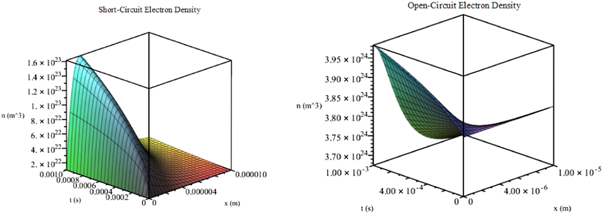
Figure 6. Exact solution n(x, t) for (41) under short-circuit conditions (left) and open-circuit conditions (right).
Download figure:
Standard image High-resolution image3.3. Nonlinear case
Based on the Lie symmetry analysis carried out by Maldon et al in their 2020 paper, we find that physically relevant versions of the nonlinear PDE (39) do not exhibit symmetry solutions [5]. Thus, we solve this equation numerically, as shown in [40, 66]. In [67], we solve equation (39) with the boundary conditions (40) using a forward time continuous space finite difference scheme. All simulations use 100 spatial nodes and 100, 000 temporal nodes with constant values taken from table 3.
In figure 7, we see that the numerical solution greatly resembles the exact solution for the linear case, suggesting that nonlinear diffusion only affects the overall magnitude of the solution. Nevertheless the nonlinear diffusion coefficient significantly lowers the overall electron density, corresponding to stronger traps in the  semiconductor [68].
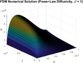
Figure 7. Numerical Solution for n(x, t) for the case of nonlinear diffusion with β = 1.
Download figure:
Standard image High-resolution image3.4. Effect of parameters on electron density
We investigate the effect of the parameters μ, ν and ξ on the solution profile for the linear case β = 1 as given by (39).
In figure 8, we plot the numerical solution for t = 1 for the electron density to elucidate the effect of β. We see that higher values of β lead to an overall decrease in electron density. Furthermore, numerical solutions reach an equilibrium faster with increased values for β. Given that β governs the density of trap states in a DSSC (higher values of β leading to deeper traps [40]), this result shows that the nonlinear diffusion mechanism is functioning in equation (39) as expected.

Figure 8. Plot of n(x, 1) for various values of β.
Download figure:
Standard image High-resolution imageFigure 9 shows the relationship between μ and the electron density. By varying μ by several powers of 10, we see that the increase in values of μ leads to a significant overall increase in electron densities. This is as expected since μ is the main coefficient in the source term  .
.

Figure 9. Plot of n(x, 1) for various values of μ.
Download figure:
Standard image High-resolution imageNext, we consider the effect of ν on the electron density. For this study, we run simulations varying values of ν by different multiples of the original value in table 3. Since  , an increase in ν leads to a decrease in the electron generation, which in turn decreases the electron density as we see in figure 10.
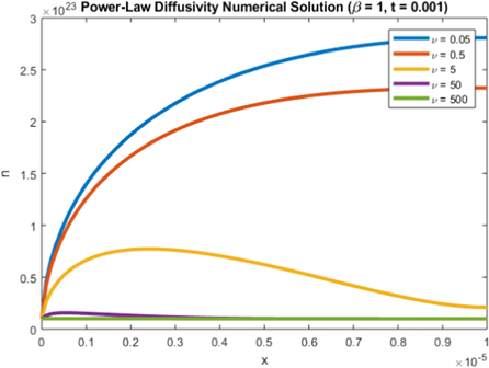
Figure 10. Plot of n(x, 1) for various values of ν.
Download figure:
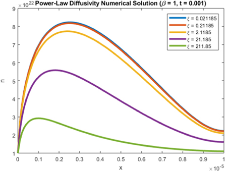
Standard image High-resolution imageFinally, figure 11 demonstrates the effect of the recombination parameter ξ on the electron density. The increased values of ξ correspond to higher levels of recombination, which is reflected in figure 11 as the electron density decreases for higher values of ξ.
Figure 11. Plot of n(x, 1) for various values of ξ.
Download figure:
Standard image High-resolution image
4. Efficiencies
According to data provided in each reference shown in table 4, we compute the nondimensional parameters μ, ν and ξ of the DSSC model.
Table 4. Nondimensional parameter values for various DSSC diffusion models.
| Author | References | μ | ν | ξ |
|---|---|---|---|---|
| Ni et al (2006) | [39] | 250 | 5 | 0.5 |
| Andrade et al (2011) | [1] | 7.292 × 10¹² | 1 | 0.385 |
| Gacemi et al (2013) | [35] | 4.861 × 10¹² | 1 | 0.385 |
| Shi et al (2013) | [51] | 6.417 × 10¹¹ | 4 | 2.5 |
| Lopes et al (2015) | [25] | 2.483 × 10¹⁹ | 1.25 | 0.602 |
| Belarbi et al (2015) | [15] | 4.327 × 10¹² | 1 | 0.385 |
The extreme values for μ are primarily due to the high values of the incident photon flux ϕ and the low values of the diffusion coefficient D0. Discrepancies between the values of μ in table 4 are largely due to the value used for the dark equilibrium electron density, neq . In Andrade et al [1], neq is given by

where n0 is the effective density of states in the DSSC, Ec is the conduction band energy and ERedox is the redox energy of the DSSC. Given that n0 = 1027 m−3, Ec − ERedox = 0.93 eV and T = 298 K, we find neq ≈ 1.87 × 10¹¹ m−3.
Alternatively, Ni et al [39] assumes that the electron density is of the order 1022m−3. This distinction primarily affects the open-circuit voltage Voc , which in turn affects efficiency η.
Table 5 shows the computed efficiency of the DSSC according to the data found for each reference. Given O'Regan and Grätzel's [4] original DSSC featured an efficiency of 7.1–7.9%, we find that the values for efficiency in table 5 generally underestimate the measured efficiency of DSSCs. In most cases, this is due to an underestimation of the short-circuit current density, given as ≈120 Am−2 by O'Regan and Grätzel [4]. Nevertheless, values for the open-circuit voltage are in good agreement with the literature, with O'Regan and Grätzel's benchmark of Voc ≈ 0.7 V.
Table 5. Values for Jsc and Voc calculated with table 4.
| Author | References | Jsc (Am−2) | Voc (V) | J0 (Am−2) | η (%) |
|---|---|---|---|---|---|
| Ni et al (2006) | [39] | 148.538 | 0.240 | 1.380 | 1.921 |
| Andrade et al (2011) | [1] | 137.134 | 0.774 | 1.128 × 10⁻¹¹ | 9.099 |
| Gacemi et al (2013) | [35] | 91.422 | 0.763 | 1.128 × 10⁻¹¹ | 5.975 |
| Shi et al (2013) | [51] | 97.914 | 0.645 | 1.188 × 10⁻⁹ | 5.291 |
| Belarbi et al (2015) | [15] | 81.366 | 0.7603 | 1.1282 × 10⁻¹¹ | 5.2940 |
| Lopes et al (2015) | [25] | 148.054 | 1.146 | 6.105 × 10⁻¹⁸ | 15.1788 |
5. Summary
In summary, we have reviewed the diffusion model for DSSCs. Modelling DSSC performance on the density of charge carriers is largely inherited from previous knowledge of solar cells but is known to be a diffusion-dominated process [22, 33].
From the electron density we calculate the short-circuit current density Jsc , the open-circuit voltage Voc and the efficiency η of a DSSC based on the diode equation. Our results for electron density are in good agreement with the literature. We analyse the electron density as a solution to equation (8) under variation in the nondimensional parameters μ, ν and ξ and provide their typical values based on data given in the literature.
Although some values are in line with literature benchmarks, there is plenty of scope for improvement. Few DSSC models consider the impact of the electrolytes and the counter electrode on the overall electron density. Moreover, these models additionally opt for steady-state measurements. To improve DSSC models, we suggest expanding the PDE given by (8) to include the effect of the counter electrode and the electrolytes. Finally, given the fractal geometry of the nanoporous semiconductor  , we also suggest a fractional diffusion equation in a similar vein to Nigmatullin [69].
Acknowledgments
The authors acknowledge the support of the Australian Government Research Training Program Scholarship for BM. The authors are also grateful to the Australian Research Council for the funding of Discovery Project DP170102705.