
Abstract
The avalanche waiting time behaviour of the Chapman sandpile model (Chapman et al, 2001 Phys. Rev. Lett. 86, 2814), compared to the ELM waiting time behaviour of a JET fusion plasma, has been considered by (Bowie et al, 2016 Phys. Plasmas 23, 100 703). Here we extend the analysis of the Chapman sandpile model, by considering cases in which the combinations of variables chosen give rise to three distinct waiting times. It is observed that the short and medium waiting times sum to the long waiting time, suggesting a relationship between all three. Further, it is observed that each of the short, medium, and long waiting times occur independently. We conject that if the short and medium waiting times sum to the long waiting time in a fusion plasma, that may suggest that the Chapman model and the fusion plasma share an underlying common dynamical behaviour, and further, that each of the three waiting times may arise from the same underlying cause. By contrast, if the short and medium waiting times do not sum to the long waiting time, that suggests that the Chapman model would be inappropriate. We remark that the relationship between the short, medium, and long waiting times bears a resemblance to the relationship between the terms of the Fibonacci sequence, and is also consistent with frequency coupling.
Export citation and abstract BibTeX RIS
1. Introduction
Sandpile models [1] have been used to analyse the behaviour of fusion plasmas [2–11]. In particular, the avalanching behaviour of the sandpile model introduced by Chapman [6, 12] has been compared to the ELMing behaviour of a fusion plasma [13].
The Chapman sandpile model is a non-conservative model in which sand is gradually introduced at the centre, or core, and escapes from the edge when systemwide avalanches (called mass loss events, or MLEs) occur. Avalanches occur when the 'critical gradient' (Zc) is exceeded between adjacent cells in the sandpile. The key feature of the Chapman model is the introduction of a 'fluidization length' (Lf) over which sand is fluidized behind the critical point at which the critical gradient is exceeded, such that the total amount of sand in the Lf cells behind the critical point, together with the amount of sand in the following cell, is re-distributed evenly over those cells. As this re-distribution increases the amount of sand in the cell immediately following the critical point, sand moves from the centre to the edge when an avalanche occurs. Avalanches may terminate before reaching the edge, or they may be systemwide, resulting in an MLE. If a systemwide avalanche occurs, the sandpile is 'swept' again until no more sand falls off the edge of the sandpile.
Further sand may be added during between sweeps of the sandpile (Running Model) [13], or fuelling may be paused until the avalanche ceases, consistent with the original Chapman model [6, 12] (Classic Model). Here we consider the Classic Model. We treat the core of our model, being the location at which sand is added, as analogous to the maximum practically available penetration depth for the addition of fuelling in a fusion plasma [14].
The waiting time between MLEs (δtn) in the sandpile model has been compared [13] to waiting times between ELMs in a fusion plasma [15]. It has been observed that a fusion plasma at JET shows evidence of multiple discrete waiting times [15], and similar discrete waiting times have been observed in the sandpile model [13]. Two discrete waiting times were observed in each of the JET plasma and the sandpile model.
Here we extend the analysis of the sandpile model to those cases where three discrete waiting times are observed.
2. Three discrete waiting times
The discussion in Bowie, Dendy and Hole [13] focuses on the two primary discrete  observed in the datasets considered there, reflective of the JET fusion plasma dataset discussed by Calderon et al [15]. There is very weak evidence in the delay pdfs of Calderon et al [15] for 3 wave coupling in the transition from single periodic to doubly periodic behaviour. In this work we comment on the relevance of the third δtn observed in the datasets generated here, and the relationship between the three discrete δtn observed. The sand simulations were generated using Mathematica. In each case, we employ a 500 cell sandpile with Zc = 120, and Lf = 5, with the amount of sand, dx, added at each iteration, kept constant during each simulation. We run each simulation for 2 million iterations, which allows for sufficient time for the sandpile to load and for a significant number of MLEs to occur. We record the iteration number at which each MLE occurs, as well as the amount of sand lost from the system in each MLE. The number of iterations between successive MLE is referred to here as the waiting time, δtn. We then run further simulations in which differing values of dx are employed (although kept constant during the course of each simulation), with all other variables held constant.
First we consider a probability distribution function (pdf) for δtn, from a single sandpile simulation for dx = 1.08, as shown in figure 1, in which the existence of three discrete peaks, representing short (S), medium (M), and long (L) δtn, is seen. Waiting time behaviour depends upon dx/Zc, such that particular values of dx and Zc are not relevant [16]. We here consider only variations of dx, and hold Zc constant.

Figure 1. Probability distribution function - dx = 1.08. Three discrete δtn can be observed (marked with vertical dashed lines), at δtn = 48000, 88 000, and 140 000.
Download figure:
Standard image High-resolution imageWe can observe the combinations of the δtn for the sandpile simulation considered in figure 1 in the delay plot in figure 2, in which we plot δtn against  . This plot shows us that any of the nine possible combinations of S-S, S-M, S-L, M-S, M-M, M-L, L-S, L-M, and L-L can occur in a single dataset. The potential combinations appear at the vertices of the dashed lines which represent
  and 140 000.

Figure 2. Delay plot, δtn against  , for dx = 1.08. Each combination of S, M, and L δtn is observed. The size of the MLE is given by the colour (blue—smallest) and size (logarithmic scale) of the bubbles. Consistent with figure 1, vertical and horizontal dashed lines represent δtn = 48000, 88 000, and 140 000 and
  and 140 000, respectively.
Download figure:
Standard image High-resolution imageA combined delay plot is shown in figure 3. Each colour in the combined delay plot represents a different value of dx. MLE size is also represented by the size of the circles, on a logarithmic scale. The possible combinations of S, M, and L can be observed in figure 3 represented by the distinct lines of data points starting at the origin—S-M, S-L, and M-L are represented by the upper line, S-S, M-M, and L-L are represented by the centre line, and L-S, M-S, and L-M are represented by the lower line. The linear relationship between  and Zc can also be observed, as each of the three distinct δtn become shorter as fuelling increases, i.e., as you move towards the origin. A simple explanation for the behaviour of all three peaks as fuelling increases may be that the faster the sandpile is loaded, the more quickly it will reach a critical state in which a systemwide avalanche occurs.
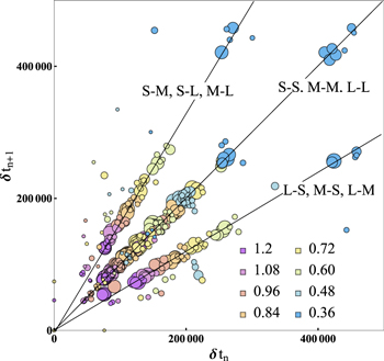
Figure 3. Combined delay plot for dx = 0.36, dx = 0.48, dx = 0.6, dx = .72, dx = .84, dx = .96, dx = 1.08, and dx = 1.2. Each colour represents δtn for a single  value, the values of which are shown in the legend. Shorter δtn corresponding to higher values of
  , and appear in the bottom left hand corner of the plot. Smaller bubbles represent smaller MLEs, on a logarithmic scale.
Download figure:
Standard image High-resolution imageFigure 4 gives the pdf of MLE size against dx for low fuelling values. The existence of peaks in figure 4 is interesting. We note that systemwide avalanches are conditioned by the system size and therefore need not exhibit the scale-free behaviour of the internal (non-MLE) avalanches. The pdfs are of a common form, and unlike the δtn pdfs, the peaks do not substantially differ in position with fuelling. This suggests the amount of sand which is lost from the system in the largest MLEs does not differ significantly with fuelling. We speculate this may occur because the same amount of sand has accumulated in the system in each case, as there is an inverse relationship between fuelling and δtn.
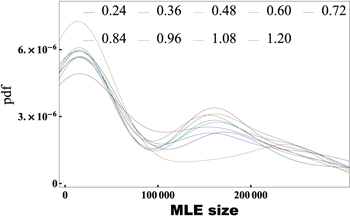
Figure 4. Combined MLE size, pdf versus MLE size, for dx = 0.24, 0.36, 0.48, 0.60, 0.72, 0.84, 0.96, 1.08, and 1.20.
Download figure:
Standard image High-resolution imageNext we compare the S, M, and L δtn represented by each of the peaks, to see whether any relationship can be observed between them.
Figure 5 shows that the sum of the δtn represented by the left and centre peaks is consistently equal to the δtn represented by the right peak, i.e., that S and M δtn together equal L δtn. This may suggest the existence of frequency coupling (in the case of the particular set of values chosen for the algorithm under consideration here).
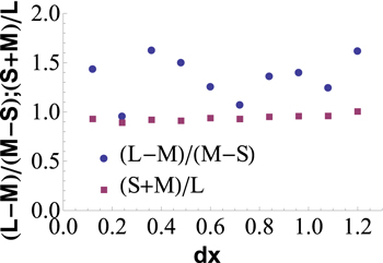
Figure 5. Relationship between left and right peaks—low dx. The purple squares represent the ratio of the sum of the left (S) and centre (M) peaks to the right (L) peak. It is notable that this ratio is approximately 1: 1, meaning that the short and medium δtn approximately sum to the long δtn. The blue circles represent the ratio of the distance between the left and centre peaks (i.e., the difference in δtn between S and M), as compared to the distance between the centre and right peaks (i.e., the difference in δtn between M and L). It is notable that while this ratio is not constant, it is approximately bounded between 1 and 1.8.
Download figure:
Standard image High-resolution imageFigure 5 also shows that while the relationship between the distances from the left to centre, and right to centre, peaks, is approximately bounded between 1.0 and 1.8, that relationship does not show a clear trend, unlike the relationship between the sum of the left and centre peaks and the right peak. This variability suggests that the relationship is not that of a simple centre peak with 'shoulders' equidistant from the centre.
Figure 6 shows that these relationships continue to be observed for higher values of dx. The 1: 1 ratio between (S + M) and L is worthy of further investigation. Two possibilities are worthy of consideration. First, that an avalanche occurring after a short δtn is merely an intermediate loss of energy prior to full system emptying at a further medium δtn - i.e., that full system emptying occurs at S + M = L, such that the avalanche occurring at S can be essentially disregarded. The second possibility is that each δtn is independent of the others, notwithstanding that S + M = L. We investigate these alternatives by considering a string of avalanches produced in a single sandpile simulation. With dx set to 0.96, we observe the sequences of δtn shown in figure 7. While we observe long sequences of M's, and a long sequence of L's, importantly, we observe that all nine combinations of S-S, M-M, L-L, S-M, S-L, M-L, M-S, L-M, and L-S appear. It is also notable that short δtn are clustered towards the beginning of the sequence and become rarer (but not non-existent) later.

Figure 6. Relationship between δtn peaks—high dx. This shows the same information as figure 5 for values of dx up to dx = 100. We observe that S and M continue to sum to L, and that  is approximately bounded between 1 and 1.8.
Download figure:
Standard image High-resolution image
Figure 7. Waiting time sequence - dx = 0.96. The lines at δtn = 55000, 97 000, and 160 000 correspond to peaks in the probability distribution function (not shown).
Download figure:
Standard image High-resolution imageWhen we set dx = 1.08, as in figures 1 and 2, we observe the sequences of δtn which are shown in figure 8. As with figures 1 and 2, horizontal dashed lines represent δtn = 48000, 88 000, and 140 000.
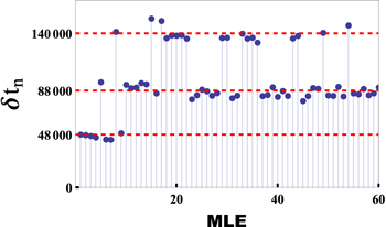
Figure 8. Waiting time sequence - dx = 1.08. The horizontal lines at δtn = 48000, 88 000, and 140 000 correspond to peaks in the probability distribution function shown in figure 1, and to the locations of the data points in the delay plot shown in figure 2.
Download figure:
Standard image High-resolution imageAgain, we see that all combinations of sequences S, M, and L appear, as also shown in figure 2, and that short δtn predominantly appear at the beginning of the sequence.
This analysis suggests that the fact that the short and medium δtn sum to the long δtn is not simply explained on the basis that in some cases a combination of short and medium δtn are substituted for a single long δtn, or that in some cases, a non-systemwide avalanche occurs giving the appearance that a long δtn has occurred. If that were so, we would expect to see S-M and L predominating in the sequence, and we would not expect to see sequences of either S or M (although we might observe sequences of L). In fact, we observe that sequences of both S and M do appear, and that S-M and L do not predominate. As a result, we conclude that S is not merely an intermediate between M and L, and that each δtn may occur independently.
It is also noteworthy that the MLE size for short δtn is smaller than for medium or long δtn. This might be taken to imply that the MLE which follows a short δtn is merely an interruption of a long δtn, and that the subsequent δtn is not substantially affected by the prior MLE, as insufficient sand is lost to make much difference to the loading time necessary for the next MLE to occur. Again, if that were the entire explanation, it would imply that only S-M and L should be seen, and that S should always precede M. As that is not observed, the small MLE size cannot be taken to be the explanation for the subsequent δtn.
An alternative proposition is that any combination of multiples of S and M may occur, producing δtn which cannot be categorised neatly as S, M or L. Such combinations are not observed, which may be because they do not occur at all, or it may be because they are highly unlikely, and simply not observed within the limits of the runtimes chosen.
Finally, we observe that the fact that S + M = L corresponds to the behaviour of the Fibonacci sequence. The Fibonacci sequence is given by  for n > 1, commencing with F0 = 0, F1 = 1, which gives 0, 1, 1, 2, 3... [17]. Normalising the sequence of δtn, such that S = 1 gives us F3 + F4 = F5, where F3 = S, F4 = M, and F5 = L.
As the ratio between consecutive terms in the Fibonacci sequence tends to the golden ratio, ϕ, if S, M, and L do represent terms in the Fibonacci sequence, then we can represent S, M, L as  , and their reciprocals as
  . Given that
  , then 1/S = 1/M + 1/L. As S, M, and L represent waiting times, their reciprocals represent frequencies (f), such that, if S, M, and L represent terms in the Fibonacci sequence, then fS = fM + fL. We show this frequency relationship in figure 9, where we see that (1/L + 1/M) ≈ (1/S), or fS ≈ fM + fL. This suggests that the relationship between S, M, and L may represent an example of frequency coupling, in which f1 = f2 + f3, consistent with non-linear behaviour seen in other plasma contexts [18].

Figure 9. Frequency sum - dx versus  . This reports the same data as shown in figure 6, using frequency relationships rather than waiting time relationships. We observe that
  , for the range of values of dx shown here.
Download figure:
Standard image High-resolution image
3. Conclusions
If this analysis is extended to the waiting times between ELMs in a fusion plasma, it suggests that similar behaviour, in which short and medium waiting times between ELMs sum to the longest waiting time, may be observed in particular cases. In the event that such behaviour is observed, our analysis suggests that it may be attributed to a single cause, rather than seeking separate causes for each waiting time. This would be particularly so in the event that the relationships of the three  are similar to those observed here, namely that the short and medium δtn sum to the long δtn. By contrast, if three distinct waiting times are observed, and the short and medium waiting time do not sum to the long waiting time, that would tend to imply that separate causes should be sought for each distinct waiting time. There is some weaker evidence to support the proposal that where the short and medium waiting times do not sum to the long waiting time, this may indicate that these waiting times have multiple underlying causes, rather than a single underlying cause. Finally, we observe that this relationship of S + M = L is consistent with the terms of the Fibonacci sequence, and is also consistent with frequency coupling.
Acknowledgments
This work was jointly funded by the Australian Research Council, through grants FT0991899 and DP170102606, and the Australian National University. One of the authors, C A Bowie, is supported through an ANU PhD scholarship, an Australian Government Research Training Program (RTP) Scholarship, and an Australian Institute of Nuclear Science and Engineering Postgraduate Research Award.