Article

A 1% Measurement of the Gravitomagnetic Field of the Earth with Laser-Tracked Satellites

1
Istituto di Astrofisica e Planetologia Spaziali (IAPS)—Istituto Nazionale di Astrofisica (INAF), Via Fosso del Cavaliere 100, Tor Vergata, 00133 Roma, Italy
2
Istituto di Scienza e Tecnologie dell’Informazione (ISTI)—Consiglio Nazionale delle Ricerche, Via G. Moruzzi 1, 56124 Pisa, Italy
3
Istituto Nazionale di Fisica Nucleare, Sezione di Roma Tor Vergata, Via della Ricerca Scientifica 1, 00133 Roma, Italy
4
Dipartimento di Fisica, Università di Roma Tor Vergata, Via della Ricerca Scientifica 1, 00133 Roma, Italy
*
Author to whom correspondence should be addressed.
Universe 2020, 6(9), 139; https://doi.org/10.3390/universe6090139
Submission received: 16 July 2020 / Revised: 24 August 2020 / Accepted: 26 August 2020 / Published: 31 August 2020
(This article belongs to the Special Issue Frame-Dragging and Gravitomagnetism)

Abstract

:
A new measurement of the gravitomagnetic field of the Earth is presented. The measurement has been obtained through the careful evaluation of the Lense-Thirring (LT) precession on the combined orbits of three passive geodetic satellites, LAGEOS, LAGEOS II, and LARES, tracked by the Satellite Laser Ranging (SLR) technique. This general relativity precession, also known as frame-dragging, is a manifestation of spacetime curvature generated by mass-currents, a peculiarity of Einstein’s theory of gravitation. The measurement stands out, compared to previous measurements in the same context, for its precision ( 7.4 × 10 3 , at a 95% confidence level) and accuracy ( 16 × 10 3 ), i.e., for a reliable and robust evaluation of the systematic sources of error due to both gravitational and non-gravitational perturbations. To achieve this measurement, we have largely exploited the results of the GRACE (Gravity Recovery And Climate Experiment) mission in order to significantly improve the description of the Earth’s gravitational field, also modeling its dependence on time. In this way, we strongly reduced the systematic errors due to the uncertainty in the knowledge of the Earth even zonal harmonics and, at the same time, avoided a possible bias of the final result and, consequently, of the precision of the measurement, linked to a non-reliable handling of the unmodeled and mismodeled periodic effects.

1. Introduction

The theory of General Relativity (GR) [1,2,3] in over a century since its formulation has brilliantly passed many experimental and observational tests, and it presently represents our best understanding of gravitation. In fact, GR is a revolutionary, very profound, and elegant theory for the description of the gravitational interaction that interprets gravity as a manifestation of spacetime curvature. Among the many predictions of Einstein’s geometrodynamics, a very peculiar role is played by Gravitomagnetism [4,5,6,7], which shows us the greater richness of GR compared to Newton’s theory of universal gravitation. Indeed, gravitomagnetism describes gravitational phenomena that are analogous to the magnetic effects of Maxwell’s theory of electromagnetism. This analogy is quite stringent in the so-called weak-field and slow-motion (WFSM) limit of Einstein’s GR. This limit implies: G M / r c 2 1 , J / M r c 1 , and v / c 1 , where G, M, and J represent, respectively, the gravitational constant, the mass of the primary and its intrinsic angular momentum, c and v are the speed of light and that of the satellite, while r represents the satellite distance from the primary. Following this approach, we have a gravitoelectric field E G E produced by masses, analogous to the electric field produced by charges, and a gravitomagnetic field B G M produced by mass-currents, analogous to the magnetic field produced by electric currents. This is gravitoelectromagnetism [8]. Therefore, GR predicts a formal counterpart to the Ampère’s law describing the magnetic effects that are related to the electric currents [9], which does not have an analogous counterpart in Newton’s theory, that (as is well known) has only a counterpart in Coulomb’s law of electrostatics.
Gravitomagnetism describes the gravitational effects that are produced by mass-energy currents. This points to its fundamental role in explaining high energy astrophysical phenomena, as a powerful source in creating (together with magnetohydrodynamic phenomena) the accretion disks and the jets observed in quasars and active galactic nuclei (AGN), due to the presence of a rotating supermassive black hole in their centers [10,11,12,13,14,15,16]. Currently there is not yet an observational direct evidence of the role of gravitomagnetism in the strong-field regime, as the one highlighted above. Nevertheless, in the WFSM limit of GR, two different kind of measurements have been done of the gravitomagnetic field produced by the Earth1.
One of these measurements was achieved by the NASA and Stanford University space mission denominated Gravity Probe B (GP-B) [22,23]: a gyroscope in polar orbit around the Earth is subject to two main relativistic precessions, a drift in the orbital plane, i.e., the de Sitter effect or geodetic precession [24], and a frame-dragging effect perpendicular to the orbital plane [25,26,27,28]. This frame dragging, also known as Pugh-Schiff dragging, is due to the Earth’s rotation, i.e., to gravitomagnetism. GP-B has provided a measurement of the frame-dragging effect and of the geodetic effect in agreement with the GR predictions with accuracies of about 19% and 0.28%, respectively. GP-B has been an independent and unique experiment, very beautiful, but also quite expensive, and unfortunately without any possibility of replicating it in the foreseeable future. The original goal of GP-B was a ≈1% measurement of gravitomagnetism [29].
The second kind of measurement was based on the measurement of the Lense-Thirring effect on the orbits of passive laser-ranged satellites, as the two LAGEOS [30,31,32,33,34,35], and, more recently, also including the orbit of LARES [36,37,38,39,40,41,42]. The Lense-Thirring effect is the precession of the orbit of a satellite around a primary due to the angular momentum (or spin) of the primary itself [43,44]. Contrary to the case of GP-B, these measurements may be repeated many times, allowing for replicability of the experiment from different research groups, with different software for the data analysis, modeling procedures and also using a different methodology in the evaluation of the error budget of the measurement [45,46]. Indeed, although the measurements of the Lense-Thirring effect with the analysis of the orbit of laser-tracked satellites has been subject to a number of criticisms in the past [34,47,48,49,50,51,52], their error budget, in terms of the evaluation of the main systematic sources of error, provides an error level smaller than that of GP-B.
In this paper, we present a new precise and accurate measurement of the Lense-Thirring effect on the combined orbits of the geodetic satellites LAGEOS, LAGEOS II and LARES. This work aims to complement and further extend the results of [41], which were based on a number of new features with respect to previous measurements. These mainly concern (i) the dynamical model used for the gravitational field, (ii) the way to perform the measurement of the relativistic effect from the analysis of the combined orbits of the satellites, (iii) the concomitant estimate of the low-degree coefficients of the Earth’s gravitational field with the unmodeled relativistic precession, and, finally, (iv) the accurate estimate of the systematic errors of the measurement.
This work is part of the activities of the LAser RAnged Satellites Experiment (LARASE) [46] and concludes these activities for what concerns the measurement of the Lense-Thirring effect. Other objectives of LARASE, in the field of fundamental physics measurements [53,54], will flow into the new experiment SaToR-G (Satellites Tests of Relativistic Gravity). The main goal of SaToR-G is to tests relativistic gravity in the WFSM limit and compare the predictions of GR with those of other alternative theories for gravitation to search (possibly) for new physics beyond GR [55,56].
The paper is organized as follows. In Section 2, the precessional effects that are produced by the gravitomagnetic field are briefly introduced with a discussion on the importance of a reliable measurement of gravitomagnetism. In Section 3, the main results regarding the Lense-Thirring effect are concisely mentioned with the estimate of their error budget. In Section 4, we will focus on errors deriving from imperfect knowledge of Earth’s gravitational field and how they have been handled by a careful consideration of their time dependence. In Section 5, the analyses undertaken to perform the relativistic precession measurement will be described. In Section 6, we present the results regarding the measurement of the Gravitomagnetic field of the Earth through the measurement of the Lense-Thirring parameter μ in two cases: from the residuals of μ obtained from the joint analysis of the orbits of the satellites and from their integration. In Section 7, the measurement of the relativistic parameter is presented in a statistical context, in order to decorrelate the measurement of the secular effect from the periodic terms not modeled in the data reduction and estimate (in an alternative way) their impact on the measurement itself. Finally, in Section 8, we provide our conclusions on the measurement we performed.

2. Lense-Thirring Effect and the Importance of an Accurate Measurement of the Gravitomagnetic Field

In the WFSM limit of GR, the precession of a gyroscope with respect to the asymptotic reference frame of distant stars can be written as:
Ω ˙ G M = 1 2 c B G M = G c 2 r 3 3 ( S · r ^ ) r ^ S ,
where S represents the spin of the primary. This particular precession is known as “dragging of gyroscopes” or “dragging of inertial frames”, as Einstein named it2. Indeed, local inertial frames have a peculiar role in Einstein’s theory of GR. These are the frames where locally, in space and, in time, the law of physics are those of special relativity and the Einstein Equivalence Principle (EEP) holds. EEP is at the basis of all metric theories of gravity, that is to those theories that, like GR, states that gravitation is a curved spacetime phenomenon. Consequently, in GR, the local inertial frames are not simply determined by the distribution of matter, but they are influenced by the distribution-and-flow of mass-currents and mass-energy in the Universe. Therefore, the gravitomagnetic field associated with these phenomena exerts a force (in Newtonian words) on moving bodies and changes the spacetime structure produced by the gravitoeletric field by participating in generating the curvature of spacetime.
In 1918, Thirring [43] and Lense & Thirring [44] computed the drag exerted by the spin of a central body, like a planet, on an orbiting moon3. They computed the secular rates of the longitude of pericenter and of the right ascension of the ascending node for some of the moons of the Solar System: indeed, the orbital plane of the moon can be seen as a sort of enormous gyroscope dragged by the planet’s gravitomagnetic field4. Therefore, the intrinsic angular momentum of the planet, which plays the role of mass-current, according to GR curves spacetime and induces an effect on the orbit of a satellite which does not have a counterpart in the Newtonian theory.
Consequently, an accurate and reliable measurement of the gravitomagnetic field of the Earth is not only important per se, as a further and robust test of the GR predictions in the WFSM limit. There are at least three main issues that, for their importance, require a much more precise and accurate measurement of gravitomagnetism, even in weak-field conditions as the one that is considered in this paper:
  • intrinsic gravitomagnetism;
  • strong fields and compact objects; and,
  • Mach’s principle.
These are briefly discussed here.

2.1. Intrinsic Gravitomagnetism

Intrinsic gravitomagnetism describes the spacetime curvature effects related with mass-currents, and not simply the corresponding effects that depend on the motion of a body on a static background field. This, in a nutshell, describes the main difference between the de Sitter [24] precession, which depend on the mass, and the Lense-Thirring precession, which depend on the angular momentum [5,60].

2.2. Strong Fields and Compact Objects

Two issues of modern astrophysics that require, for their explanation, the contribution of GR, are the mechanisms at the basis of the accretion of matter around compact objects and those of acceleration of charged particles in sources of various nature and size, with the simultaneous emission of powerful radio jets. Currently, the nature of the accretion mechanisms as well as that of the acceleration of particles and of the emission of relativistic jets is largely unknown under many aspects.
The classical physical processes presently considered as driving the interaction of the flow of matter with the central compact object, still require the correct inclusion, in the models developed to describe the details of the interaction, of the relativistic mechanisms that are produced by the gravitomagnetic field of the rotating compact object. These relativistic effects produce a dragging of the accretion disk and the alignment of the radio jets with the spin of the compact object [10,11,12,13,14,61]. Numerical relativity plays a major role in this context but, to our knowledge, papers that focus explicitly on the contribution due to the gravitomagnetic effects are not available in the literature.

2.3. Mach’s Principle

Mach’s ideas on the origin of inertia and on the relativity of rotation [62], as in the discussion regarding the well-known bucket experiment by Newton, strongly influenced Einstein in the development of GR. Mach was very precise and clear on these aspects: there is no absolute space and the Newtonian concept of acceleration has only meaning with respect to the very distant stars. Consequently, Mach is implicitly referring to a cosmological context. Again, in a nutshell, the sentence “inertia here arises from mass-energy there” [5] summarizes very well the meaning of gravitomagnetism and makes us interpret the Lense-Thirring effect (i.e., the dragging of inertial frames) as a weak GR formulation of the ideas of Mach, which is of what Einstein called Mach’s Principle [1,63,64]. For further details on the relationship between the Mach’s Principle and the Lense-Thirring effect, we refer to [65,66]. Concerning the cosmological implications of Mach’s Principle, these are complex, still debated and theory-dependent. We refer to the literature for further details, see e.g., [5,57,67,68,69].

3. On Past and Recent Measurements of the Lense-Thirring Effect

To this date, we lack an observational direct evidence of the gravitomagnetic effects in the strong field regime. On the other hand, in the WFSM limit of GR, several different works have successfully provided a measurement of the gravitomagnetic field produced by the Earth [22,23,30,33,34,36,37]. In fact, as we have already highlighted, the precession of the orbital plane of an Earth-bound satellite that is caused by the so-called Lense-Thirring effect [43,44] represents one of the most peculiar predictions of Einstein’s theory of GR related to gravitomagnetism. The orbital plane of the satellite behaves, in principle, as an external inertial frame not bound to the Earth and dragged by its rotation; such dragging is observable if the classical disturbances due to the main gravitational and non-gravitational perturbations are properly modeled during the precise orbit determination (POD), or can be removed a posteriori, or considered to be negligible on the time span of the orbital analysis.
The dragging effect manifests itself in a secular shift of the right-ascension of the ascending node (RAAN) Ω and of the argument of pericenter ω of the considered satellites [44]:
Ω ˙ LT = μ 2 G J c 2 a 3 ( 1 e 2 ) 3 / 2 = μ K LT ,
ω ˙ LT = μ 6 G J c 2 a 3 ( 1 e 2 ) 3 / 2 cos i = 3 μ K LT cos i ,
where a, e, and i represent, respectively, the semi-major axis, the eccentricity and the inclination of the orbit, and J represents the angular momentum of the Earth. The dimensionless coefficient μ represents the Lense-Thirring effect parameter, with μ = 1 if GR is the correct theory of gravitation, and μ = 0 in Newtonian physics. Unfortunately, the measurements performed before 2018 had however a number of systematic errors that limited their accuracy well above 1%.
In the case of GP-B, the direct effect on an orbiting gyroscope has provided a measurement of frame-dragging with an accuracy of about 19% [22,23], after an intense and extended analysis effort needed to remove unexpected disturbances due to electric patch effects. This prevented the team to reach the original goal of 1%. Conversely, in the case of the measurements performed so far with the LAGEOS satellites [33,34,35], and also in the case of the first measurements that have included the LARES satellite [36,37], the main limitation in the accuracy of the measurement was provided by the uncertainties in the knowledge (and modeling) of the even zonal harmonic coefficients of the Earth’s gravitational potential. The accuracy of the previously cited measurements of the LT effect with laser-ranged satellites, was estimated in the 5–10% range, but gave rise to a vibrant debate in the literature [34,47,48,49,51,52].
One of LARASE’s key, albeit intermediate, objectives was to improve the modeling of the orbits of the three satellites, with the ultimate goal of refining the results that can be achieved in testing the gravitational interaction [37,40,46]. These improvements concern the modeling of both gravitational and non-gravitational perturbations [40,46,70,71,72,73,74,75,76]. In this regard, at the end of 2017, within the LARASE experiment, we started a series of analyses that aimed to improve the modeling of the gravitational field of the Earth and, in particular, the contribution of the even zonal harmonics coefficients C ¯ , 0 (i.e., those with degree = even and order m = 0 ) and of their uncertainties. In fact, these coefficients are responsible for a secular effect on Ω and ω , as that produced by the Earth’s gravitomagnetism, see Section 4. The analysis, at first tested on the first three even zonal harmonics [38,40,77], was later extended to the even zonal harmonics up to degree = 30 [41,72]. In these new analyses, we exploited the monthly solutions for the Earth’s gravitational field coefficients from the GRACE mission [78]. This allowed for us to considerably improve the accuracy of the measurement of the Lense-Thirring effect, strongly reducing the impact of the uncertainties of the even zonal harmonics in the final measurement of the relativistic precession. These aspects will be described in detail in Section 4. We obtained an error of about 2.3% in [40], and then reduced to about 1.6% in [41], both computed in a root-sum-square fashion. A similar result, about 2% in accuracy, has been obtained by [42].
Table 1 and Table 2 show, respectively, the mean orbital elements of the satellites and the expected relativistic Lense-Thirring precession on their orbits. These mean Keplerian elements have been determined by a dedicated analysis of the orbits of the satellites [46].
In the following, we will focus on the RAAN Ω as observable for the measurement of the relativistic precession. The pericenter ω of the satellites is influenced, especially for the two LAGEOS, by the effects of thermal thrust. A significant activity for the development of new models for the thermal forces—that allow us to recover the pericenter of the satellites and, in particular, that of LAGEOS II—has been carried out in recent years [73,75,79,80]. Preliminary results are encouraging and we plan to adopt them in future analyses.

4. On the Accuracy of the Even Zonal Harmonics

The gravitational potential V of the Earth is usually expanded in series of spherical harmonics in order to account for the non-uniform distribution of the mass of our planet. Concerning the contribution of the even zonal harmonics coefficients, C ¯ , 0 , to the geopotential, this may be written as [81,82]:
V , 0 = G M r = 2 R r P , 0 ( sin φ ) C ¯ , 0 ,
where φ is the geocentric latitude, R and M are, respectively, the mean equatorial radius and the mass of the Earth, r the geocentric distance, while P , 0 ( sin φ ) are the Legendre polynomials. The deviation from the spherical symmetry for the mass distribution of the Earth, described by these harmonics, is responsible for a classical precession of the RAAN of the satellite orbit, and with much larger amplitudes than Lense-Thirring precession. For instance, the secular effect in the rate of the RAAN due to the first two even zonal harmonics is [81]:
Ω ˙ class = 3 2 n R a 2 cos i 1 e 2 2 5 C ¯ 2 , 0 + 15 8 R a 3 ( 7 sin 2 i 4 ) ( 1 + 3 2 e 2 ) ( 1 e 2 ) 2 C ¯ 4 , 0 = K 2 , 0 C ¯ 2 , 0 + K 4 , 0 C ¯ 4 , 0 ,
where C ¯ 2 , 0 and C ¯ 4 , 0 are the normalized Stokes coefficients of the quadrupole and octupole moments of the Earth and n = G M / a 3 is the satellite mean motion. The order-of-magnitude of this classical precession is about +126 deg/yr for LAGEOS, −231 deg/yr for LAGEOS II, and about −624 deg/yr in the case of LARES. Thus, in order to avoid a large systematic error in the measurement of the Lense-Thirring precession, we started a careful analysis of the Earth’s multipolar moments and of their dependence on time [83,84,85,86]5. The first steps in this direction were taken in [40] in the case of the quadrupole coefficient that is responsible for the largest effect; in [41] we extended those actions to multipole coefficients of higher order, up to degree = 30 6. As mentioned above, in this work, we take up, extend, and complete these considerations.
Part of these improvements were made possible by the new solutions of the Earth’s gravitational field provided, especially, by the GRACE space mission. The twin GRACE satellites, launched on March 2002 by NASA and DLR, have provided a much improved determination of the Earth’s gravitational field, both in its static and dynamical components [78,87,88,89], with respect to previous results based on multi-satellite data. Moreover, the correlations among various coefficients, in particular the even zonal ones, have been reduced with respect to previous models, such as EGM96 [90].
In our analyses, we considered the monthly solutions7 for these coefficients provided by three independent analysis centers: CSR, GFZ, and JPL8. We then fitted these coefficients with a linear trend on the time span of our analysis, about 6.5 years, modeling each even zonal harmonic between = 2 and = 20 with the expression9:
C ¯ , 0 ( t ) = C ¯ , 0 ( t 0 ) + C ¯ ˙ , 0 ( t t 0 ) ,
where t 0 represents a reference epoch. In the Lense-Thirring effect measurements prior to 2019, only the quadrupole and octupole coefficients where modeled, by means of a linear trend [91]10. The linear trend “follows”, on average, the more complex time dependence of these coefficients, which are also characterized by the mentioned annual and semi-annual periodicities, plus other subtler periodic effects [85,92]. This approach strongly reduces the discrepancies between the effective time behavior of these coefficients and the models that use static values for the same coefficients.
It is important to stress that the static models provide values for the coefficients of the Earth’s gravity field that are averages on the time span of GRACE data. However, in different subintervals of the entire period of GRACE data, as in the case of our analysis, which starts after the launch of the LARES satellite, these average values may be quite different compared with their effective time behavior provided by GRACE monthly solutions.
In Figure 1, we exemplified, for the case of the coefficient C ¯ 20 , 0 , the procedure that we adopted to model the even zonal harmonics up to = 30 . First, we compared the time behavior of each coefficient obtained from GRACE data with the corresponding static value provided in GGM05S. This is our main reference model for the gravitational field of the Earth, see Section 5. In general, the value provided by GGM05S represents (as highlighted) an average—in the time interval over which the gravitational field has been determined—of the time-dependent values obtained from the GRACE mission. However, this overall average value is, in general, far from the average value valid in the time span of our analysis, which starts after the launch of LARES, in February 2012. Moreover, as we can see from the figure, a simple average for the coefficient over the time span of the analysis, is not generally able to capture the time evolution of the coefficient, which is better described by a linear fit to the GRACE-derived coefficients.
Hereinafter, as usual practice in this kind of analysis, we estimated, together with the relativistic precession, the corrections to the quadrupole C ¯ 2 , 0 and octupole C ¯ 4 , 0 coefficients, (by solving Equations (7) below); these are the coefficients that most contribute to the systematic errors, if not properly accounted for in the POD of the satellites; practically, the value for μ is independent of the errors related to the imperfect knowledge of these coefficients (see Section 6). We also explicitly computed the correlation of these coefficients with the relativistic parameter μ .
In the next section, we apply our considerations and analyses to several models for the background gravitational field of the Earth, in order to extract a reliable and robust measurement of the Lense-Thirring effect, as in [41]. This allows us, once the first 10 even zonal harmonics for each field were set in agreement with GRACE monthly solutions, to highlight the variability of the systematic errors among the considered fields. Consequently, this variability is due to even zonal harmonics of higher order, as well as to the non-zonal ones (tesseral and sectorial), respectively with m and with m = . Below, we first describe the characteristics of the new analyses that we have performed, and then we present the results that were obtained for the measurement of the relativistic precession of the orbital plane of terrestrial satellites due to the gravitomagnetic field.

5. The New Analyses

We analyzed the tracking data of LAGEOS, LAGEOS II, and LARES on a time span of 2359 days (about 6.5 years), starting from 6 April, 2012 (MJD 56023). The GEODYN II [93,94] software was used for the data reduction of the SLR observations of the three satellites in the normal point format [95]. These PODs have been performed by adjusting the state-vector (i.e., position and velocity) of each satellite on an arc length of seven days, to best fit the SLR data, for an overall number of 337 arcs not causally connected. The relativistic Lense-Thirring acceleration was not included in the dynamical model of GEODYN [96]. Also the subtle thermal thrust effects due to Earth’s infrared radiation (Earth-Yarkovsky effect) and to the Sun visible radiation, modulated by the eclipses (solar Yarkovsky-Schach effect) [97], were not included in the dynamical model, because, unfortunately, the routines included in GEODYN for their modelling can only handle a fast rotation regime of the satellites, which is not longer applicable for the two LAGEOS [75,98], averaging out many relevant thermal effects11.
In our new analyses we used the GGM05S solution [85,99] as reference model for the Earth’s gravitational field12. Other models considered in this work are: EIGEN-GRACE02S (2004) [89], ITU_GRACE16 (2016) [101], and Tonji-Grace02s (2017) [102,103]. All of these models were obtained from GRACE data13. For the considered gravitational models, the first 10 even zonal harmonics were modeled with the time behavior described above, while, for the remaining harmonics, the values of each single solution were used14. For solid tides we used the Colombo’s model [104], while ocean tides were described by the GOT99.2 model [105]. Furthermore, we adhered to the ILRS recommendations (those relevant for the time span of our analyses) regarding the on-ground tracking stations [106]. These recommendations regard mainly an a posteriori correction of the SLR data to avoid (or reduce) possible systematic errors that were related to several station-dependent features such as calibration issues, a possible change of the laser frequency, or of the coordinates of the station itself (within the ITRF) because of an earthquake, for instance. Among these corrections, the station biases play a special role, in particular the so-called range bias, which is correlated with the satellite center-of-mass correction [107]. We remark that the considered time span, about 6.5 years, is close to twice the period of the node of LAGEOS (1052 days), four times the period of the node of LAGEOS II (570 days) and 11 times that of LARES (211 days). This allows us to reduce the impact on the relativistic measurement of all the unmodeled (or poorly modeled) effects related to the non-gravitational and gravitational perturbations that are characterized by these periodicities. For instance, this is the case for some thermal thrust perturbations [97], or of the long-period ocean tide K 1 [71]. In the following sections, the most significant results obtained from the analysis of the residuals in the RAAN of the three satellites are described.

6. The Measurement of μ

Our observable for the measurement of the Lense-Thirring effect is represented by the RAAN Ω of the three satellites, as anticipated at the end of Section 3. Furthermore, as discussed with some details in Section 4, since the main effects that limit the measurement of the relativistic precession are the uncertainties in the knowledge of even zonal harmonics coefficients C ¯ , 0 , in particular of the first two coefficients, we have solved (separately for each arc) a system of three equations in the three unknowns δ C ¯ 2 , 0 , δ C ¯ 4 , 0 , and μ (following the original proposal of [108]15):
K 2 , 0 L 1 δ C ¯ 2 , 0 + K 4 , 0 L 1 δ C ¯ 4 , 0 + K L T L 1 μ = δ Ω ˙ r e s L 1 K 2 , 0 L 2 δ C ¯ 2 , 0 + K 4 , 0 L 2 δ C ¯ 4 , 0 + K L T L 2 μ = δ Ω ˙ r e s L 2 K 2 , 0 L R δ C ¯ 2 , 0 + K 4 , 0 L R δ C ¯ 4 , 0 + K L T L R μ = δ Ω ˙ r e s L R ,
In these equations16, the constant terms δ Ω ˙ r e s L 1 , δ Ω ˙ r e s L 2 and δ Ω ˙ r e s L R represent the residuals in the rate of the RAAN of each satellite determined, after the POD of their orbit, with the method described in [110]. In the left hand side of each equation, the coefficients K 2 , 0 L j and K 4 , 0 L j (with L j = ( L 1 ) LAGEOS , ( L 2 ) LAGEOS II , ( L R ) LARES ) are function of the orbital parameters a, e and i of each satellite, as explicitly shown in Equation (5)17. The three coefficients K L T L j represent the relativistic Lense-Thirring precession for the three satellites, see Equation (2) and Table 2. Finally, concerning the three unknowns of the system, the quantities δ C ¯ , 0 (with = 2 and = 4 ) represent the mismodeling of the even zonal harmonics of the background model of the Earth’s gravitational field, while μ represents the dimensionless Lense-Thirring parameter introduced in Equation (2)18. Therefore, with this solution, we can remove, from the estimate of μ , the uncertainties that are related to the knowledge of the first two even zonal harmonics19. Figure 2 shows the results for the corrections to the quadrupole and octupole coefficients, while, in Figure 3, we show the results for μ , evaluated, for each arc, as a solution of the system of Equation (7).
Figure 4, plots μ as a cumulative sum of the values shown in Figure 3. The set shown was computed using the GGM05S Earth model. The other models considered provide similar results: see below for a comparison.
To extract the Lense-Thirring parameter, we compute the mean value in the case of Figure 3, and the slope of a best fitting straight line in the case of Figure 4. It can be seen that periodic effects perturb, especially in the case of Figure 3, the measurement of the relativistic secular effect embedded in the time series of the residuals. However, we underline that the unmodeled periodic effects that characterize the residuals in Figure 3 behave—in relation of their peculiar nature that alternatively increases or decreases the unmodeled precession on various arcs—as a Gaussian (with a Skewness of 8.4 × 10 3 and Kurtosis of +3.097) superimposed to the relativistic precession.
The periodic effects that characterize the residuals in μ are due to both gravitational and non-gravitational perturbations20. However, the separation of the different effects is not simple, being influenced by the time dependence of the even zonal harmonics and, above all, by the variation of the spin of the satellites. Among the main spectral lines, we have the periodicities of the eclipses of the satellites 2 ( Ω ˙ λ ˙ ) 21, especially that of LAGEOS (about 280 days), and the periodicities, already mentioned, related to the time variation of the RAAN of the satellites Ω ˙ .
Because the cumulative sum acts as a low-pass filter, the residuals shown in Figure 4 are less influenced by the highest frequencies present in Figure 3, and allow for a cleaner, and consequently more precise, measurement of the Lense-Thirring effect. In Table 3, we show, still in the case of the GGM05S model, the correlation matrix for the three solutions of the system of Equation (7).
The correlation is particularly small between μ and the correction δ C ¯ 2 , 0 , as well as between the two corrections, δ C ¯ 2 , 0 and δ C ¯ 4 , 0 . Conversely, the correlation is moderately larger between the Lense-Thirring parameter and the correction δ C ¯ 4 , 0 . The relative low degree of correlation among the relativistic parameter μ with the corrections to the first two even zonal harmonics can be represented in the colorbar plot that is shown in Figure 5, where the values for μ are distributed in relation to those assumed by δ C ¯ 2 , 0 and δ C ¯ 4 , 0 .
This analysis provides better (smaller) correlations with respect to a previous measurement [40], where the Lense-Thirring effect was estimated together with the corrections to the quadrupole and hexapole, δ C ¯ 6 , 0 , coefficients22. Similar results are found when using all other gravitational fields. This is due to the common use we made, among the considered gravitational fields, of the first 10 even zonal harmonics estimated from GRACE monthly solutions. This is well represented in Figure 6, where the comparison among the results that were obtained for the Lense-Thirring parameter for the various models considered is shown.
That is to say, when the even zonal harmonics are well modeled in the POD of the different satellites, in the sense of considering for their dependence on time a model as close as possible to the temporal trend of these coefficients as measured by the monthly solutions of GRACE, the differences between the different gravitational field models tend to considerably decrease as regards the measurement of the Lense-Thirring precession.
In Table 4, we show the resulting value for the Lense-Thirring parameter μ , estimated from the slope of the linear fit to the cumulative residuals, for each of the gravitational models considered in our analyses.
We notice that, in all these analyses, the agreement with the GR prediction is at a fraction of percent. Additionally, the precision δ μ (at a 95% confidence level) is at a fraction of percent of the relativistic precession. As already highlighted, the variability of the results, actually very small, is mainly related to possible systematic differences among the different solutions for the gravitational field, due to even zonal harmonic coefficients with degree > 20 . Assuming, conservatively, for this measurement of the Lense-Thirring effect, the mean of the measured values of μ reported in Table 4, we obtain:
μ meas 1 = ( 1.5 ± 7.4 ) × 10 3 ± 16 × 10 3 ,
where the first terms within parentheses represent the measurement and its formal error, while the last term represents our estimate for the error budget, 1.6%. This error budget derives from a root-sum-square (RSS) of the main systematic effects that are related to the gravitational and non-gravitational perturbations that act on the orbits of the satellites. It accounts for the errors related to the static field (≃1.0%), to ocean tides (≲0.6%) 23, to other periodic effects (≃1.0%) and to the error related to the knowledge of the de Sitter precession (≃0.3%). Conversely, if we pessimistically consider the sum of the absolute values of these errors, the error budget increases to about 2.9%.

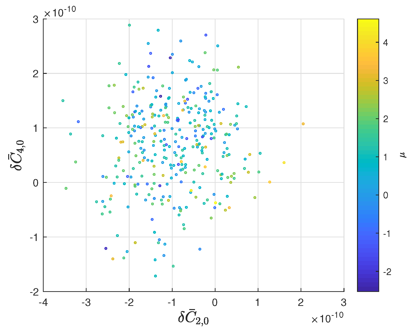
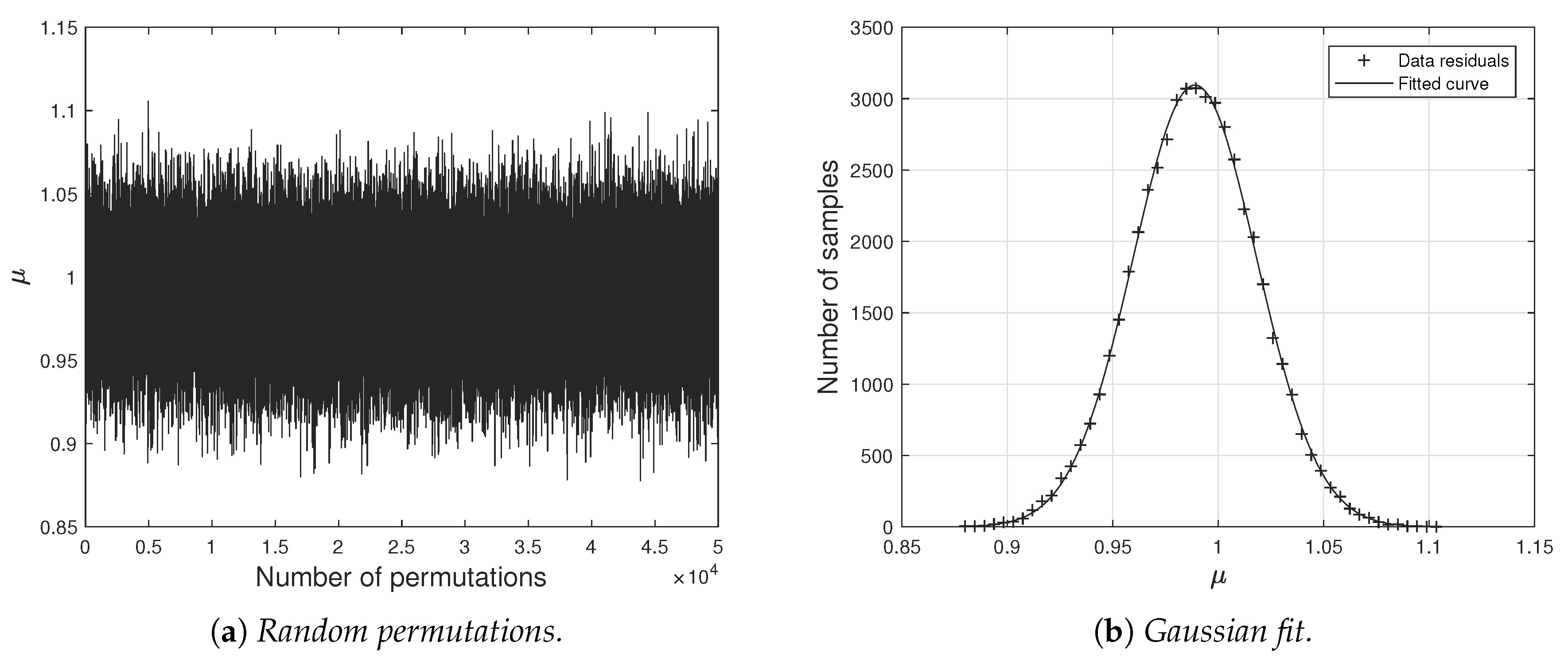
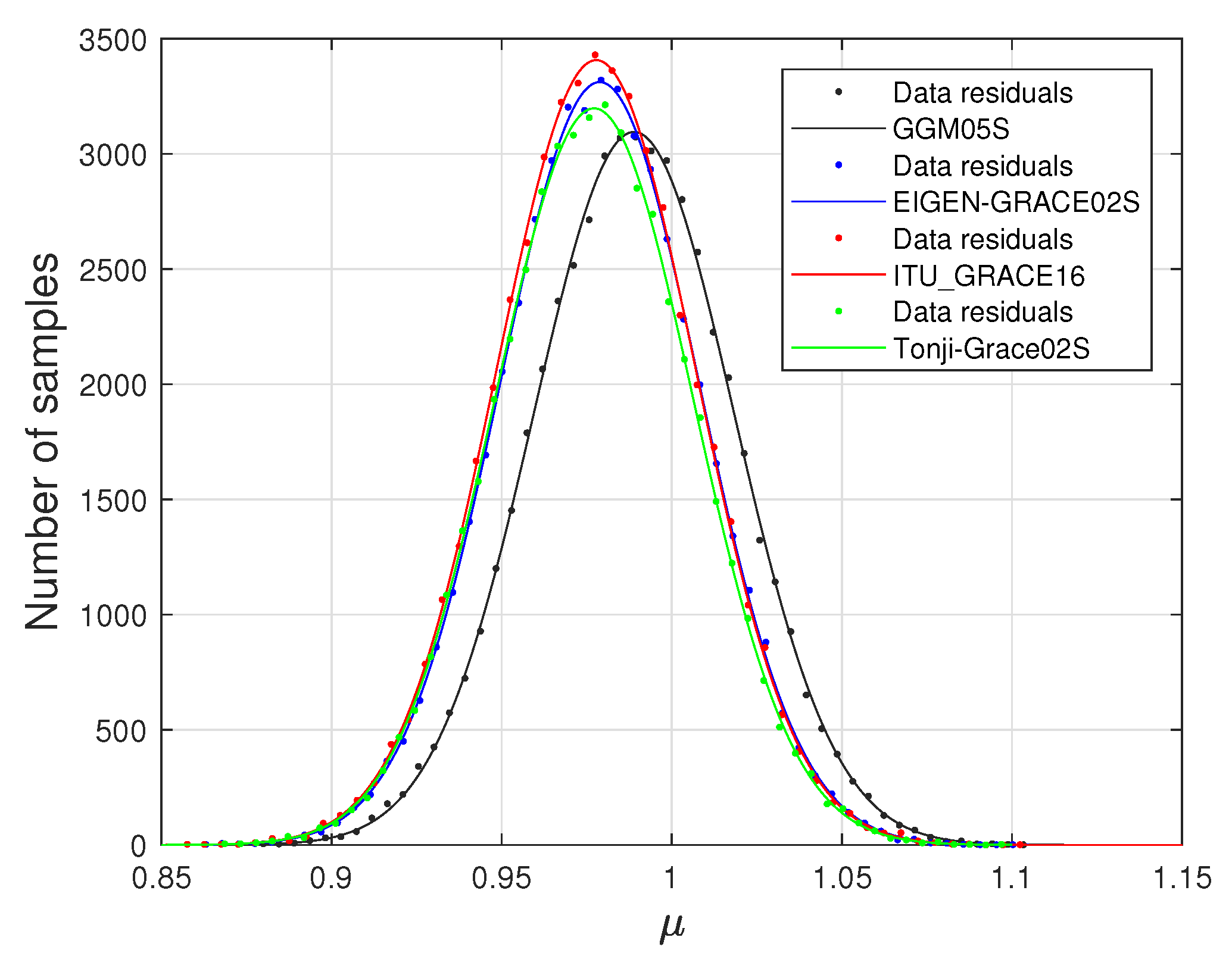
7. A statistical Approach to the Measurement of μ

Hereinafter, we consider two aspects introduced in the previous sections: the time interval of the analysis and the unmodeled periodic effects. In Section 5, we have pointed out that the time interval of our analysis has the advantage to be a integer multiple of the periods of the RAAN of the three satellites. In this case, as discussed in Section 6, the mismodeling or poorly modeling (or even the non-modeling) of some perturbation linked with these main periods has no impact in the slope of the best fitting straight line through the integrated residuals of the relativistic parameter μ . Consequently, the gravitational and non-gravitational perturbations that are characterized by these three main periods cannot be considered dangerous neither for the measurement of the relativistic effect nor for their impact in the final error budget of the measurement, i.e., for the estimate of the systematic errors. We underlined in Section 6 that the unmodeled periodic effects in the residuals of Figure 3 represent a sort of noise, with Gaussian distribution, masking the relativistic effect that represents the common (constant) signal along each arc. Of course, this periodic signal represents, in the first place, what is not modeled and which we must therefore find in the residuals. The choice of the total time interval of the analysis was made precisely to exploit this correlation, so that the main effects of some long-term perturbations mediate at zero, as explained, both in the case of the analysis of the residuals of Figure 3 and in the case of the analysis of the integrated residuals of Figure 4.
After clearing these aspects, we can estimate the impact of the periodic terms in the evaluation of the relativistic effect μ (the slope of the best fitting straight line of the integrated residuals of Figure 4 in the following way: we perform a series of random permutations of the unintegrated residuals of Figure 3, in order to decorrelate the relativistic effect present in them from the periodic effects that characterize the temporal sequence considered. For each permutation, we determine the new slope from a linear fit over the entire number of arcs. Finally, we check how the new solutions are distributed. Of course, for the Central Limit Theorem, we expect that these results are distributed very close to a Normal (i.e., Gaussian) distribution24. In Figure 7, we show the results obtained with the GGM05S model after 50,000 random permutations.
For the relativistic parameter we obtained:
μ ¯ meas 1 = ( 1.11 ± 2.94 ) × 10 2 ,
where μ ¯ meas = 0.9889 represents the mean of the Gaussian and the error represents the standard deviation σ μ of the Gaussian with a 95% confidence level. This result has a discrepancy of about 1% with respect to the result that was obtained in previous Section 6; consequently, this value confirms a 1% contribution of the unmodeled periodic terms in the overall error budget of the measurement25.
Finally, in Figure 8 and Table 5, the results for the Lense-Thirring parameter after the 50,000 random permutations are shown for the other gravitational fields considered in the present work. On average, the discrepancy in measuring μ with this statistical approach is approximately 1.9% when compared with the average result that is presented in the previous Section 6.

8. Conclusions

We presented the results of a precise and accurate measurement of the gravitomagnetic field of the Earth through the measurement of the Lense-Thirring effect on the combined orbits of the geodetic satellites LAGEOS, LAGEOS II, and LARES. These kinds of measurements raised criticisms [34,47,48,49,51,52] in the past regarding the estimate of the systematic sources of error due to the background gravitational field, which is responsible for a classical orbital precession that completely mask, if not adequately considered, the precession envisaged by Einstein’s theory of GR. We believe that the analysis reported here well overcomes these critical issues. Indeed, several new improvements have been introduced. Among these, the most significant is the modeling—in the POD of the satellites—of the even zonal harmonics of the Earth’s gravitational field through linear trends that fit the monthly solutions of the corresponding GRACE coefficients in the time interval of our analyses, about 6.5 years. We also estimated, together with the relativistic parameter μ , the corrections to the quadrupole C ¯ 2 , 0 and octupole C ¯ 4 , 0 coefficients and the correlation values among these three quantities.
These improvements have allowed us to perform the measurement by means of a simple linear fit to the orbit residuals. Indeed, whenever some of the coefficients of the gravitational field are not correctly modeled in the POD, the simple linear fit preserves the analysis from the risk of forcing the result to the desired value, using an excessive number of fitting parameters: because these could absorb some of the periodic effects beyond our ability of understanding their origin. Our final result is:
μ meas 1 = ( 1.5 ± 7.4 ) × 10 3 ± 16 × 10 3 ,
where the formal error from the fit (0.74%) has been conservatively given with a 95% confidence level. Usually, in the literature of the Lense-Thirring effect measurements, this formal error is provided at a 68% confidence level; consequently, for comparison with other recent works [40,42], our error should be rescaled to 0.38%. This result is compatible (within the errors) with the prediction of GR for the relativistic precession produced by the gravitomagnetic field of the Earth, i.e., with μ G R = 1 . The discrepancy with GR is only 0.15%, and the accuracy, calculated in RSS fashion, is 1.6%, robustly improved with respect to previous estimates.
Concerning the contribution of the unmodeled periodic effects to the error budget, the realization of a single measurement over an interval of 6.5 years has turned into 50,000 different realizations by means of the random permutation of the residuals obtained for each of the 337 orbital arcs of seven days that make up the entire period of our analysis. This allowed us to obtain a further, and independent, estimate of the errors that are related to the unmodeled periodic terms, of the order of 1%. It is clear that future work in this context will require a deeper insight and comprehension of the nature of these periodic effects in order to disentangle the contribution of the gravitational perturbations from the subtler, non-gravitational ones.

Author Contributions

D.L. and M.V. have conceived the characteristics of the measurements to be made. R.P. performed the precise orbit determination analyses. D.L. drafted the manuscript. All authors contributed to the realization of the analyses and to the revision of the manuscript. All authors have read and agreed to the published version of the manuscript.

Funding

This research received no external funding.

Acknowledgments

The authors acknowledge the ILRS for providing high quality laser ranging data of the two LAGEOS satellites and of LARES. This work has been performed by the LARASE experiment and funded by the Commissione Scientifica Nazionale (CSN2) for Astroparticle Physics of the Istituto Nazionale di Fisica Nucleare (INFN), to which we are very grateful. This work concludes the activities of the LARASE experiment [46], whose main goal was precisely to achieve a robust and reliable measure for the Lense-Thirring effect. LARASE activities will continue as regards the development of models for non-conservative forces acting on geodetic satellites. Activities in the field of fundamental physics measurements will continue in the new experiment: “Satellites Tests of Relativistic Gravity” (SaToR-G).

Conflicts of Interest

The authors declare no conflict of interest.

References

  1. Einstein, A. Die Grundlage der allgemeinen Relativitätstheorie. Ann. Phys. 1916, 354, 769–822. [Google Scholar] [CrossRef] [Green Version]
  2. Iorio, L. Editorial for the Special Issue 100 Years of Chronogeometrodynamics: The Status of the Einstein’s Theory of Gravitation in Its Centennial Year. Universe 2015, 1, 38–81. [Google Scholar] [CrossRef] [Green Version]
  3. Debono, I.; Smoot, G.F. General Relativity and Cosmology: Unsolved Questions and Future Directions. Universe 2016, 2, 23. [Google Scholar] [CrossRef]
  4. Cohen, J.M.; Mashhoon, B. Standard clocks, interferometry, and gravitomagnetism. Phys. Lett. A 1993, 181, 353–358. [Google Scholar] [CrossRef]
  5. Ciufolini, I.; Wheeler, J.A. Gravitation and Inertia; Princeton University Press: Princeton, NJ, USA, 1995. [Google Scholar]
  6. Iorio, L.; Lichtenegger, H.; Mashhoon, B. An alternative derivation of the gravitomagnetic clock effect. Class. Quantum Gravity 2002, 19, 39–49. [Google Scholar] [CrossRef]
  7. Mashhoon, B.; Hehl, F.W. Nonlocal Gravitomagnetism. Universe 2019, 5, 195. [Google Scholar] [CrossRef] [Green Version]
  8. Mashhonon, B. Gravitoelectromagnetism. arXiv 2001, arXiv:gr-qc/0311030. [Google Scholar]
  9. Ampère, A.M. Recueil d’Observations éLectro-Dynamiques; Nabu Press: London, UK, 1822. [Google Scholar]
  10. Damour, T. Black-hole eddy currents. Phys. Rev. D 1978, 18, 3598–3604. [Google Scholar] [CrossRef]
  11. Damour, T.; Hanni, R.S.; Ruffini, R.; Wilson, J.R. Regions of magnetic support of a plasma around a black hole. Phys. Rev. D 1978, 17, 1518–1523. [Google Scholar] [CrossRef]
  12. MacDonald, D.; Thorne, K.S. Black-hole electrodynamics-an absolute-space/universal-time formulation. Mon. Not. R. Astron. Soc. 1982, 198, 345–382. [Google Scholar] [CrossRef]
  13. Thorne, K.S.; Price, R.H.; MacDonald, D.A. Book-Review-Black-Holes-the Membrane Paradigm. Science 1986, 234, 224. [Google Scholar]
  14. Thorne, K.S. Gravitomagnetism, jets in quasars, and the Stanford Gyroscope Experiment. In Near Zero: New Frontiers of Physics; Fairbank, J.D., Deaver, J.B.S., Everitt, C.W.F., Michelson, P.F., Eds.; W. H. Freeman and Co.: New York, NY, USA, 1988; pp. 573–586. [Google Scholar]
  15. Remo, R.; Costantino, S. Nonlinear Gravitodynamics: The Lense-Thirring Effect; World Scientific Publishing Company: Singapore, 2003. [Google Scholar]
  16. Stella, L.; Possenti, A. Lense-Thirring Precession in the Astrophysical Context. Space Sci. Rev. 2009, 148, 105–121. [Google Scholar] [CrossRef]
  17. Deng, X.M. Preliminary investigation of the gravitomagnetic effects on the lunar orbit. In A Giant Step: From Milli- to Micro-Arcsecond Astrometry; Jin, W.J., Platais, I., Perryman, M.A.C., Eds.; Cambridge University Press: Cambridge, UK, 2008; Volume 248, pp. 399–400. [Google Scholar]
  18. Iorio, L. Analytically calculated post-Keplerian range and range-rate perturbations: The solar Lense-Thirring effect and BepiColombo. Mon. Not. R. Astron. Soc. 2018, 476, 1811–1825. [Google Scholar] [CrossRef] [Green Version]
  19. Farrugia, G.; Said, J.L.; Finch, A. Gravitoelectromagnetism, Solar System Tests, and Weak-Field Solutions in f (T,B) Gravity with Observational Constraints. Universe 2020, 6, 34. [Google Scholar] [CrossRef] [Green Version]
  20. Iorio, L. Juno, the angular momentum of Jupiter and the Lense-Thirring effect. New Astron. 2010, 15, 554–560. [Google Scholar] [CrossRef] [Green Version]
  21. Iorio, L.; Lichtenegger, H.I.M.; Ruggiero, M.L.; Corda, C. Phenomenology of the Lense-Thirring effect in the solar system. Astrophys. Space Sci. 2011, 331, 351–395. [Google Scholar] [CrossRef] [Green Version]
  22. Everitt, C.W.F.; Debra, D.B.; Parkinson, B.W.; Turneaure, J.P.; Conklin, J.W.; Heifetz, M.I.; Keiser, G.M.; Silbergleit, A.S.; Holmes, T.; Kolodziejczak, J.; et al. Gravity Probe B: Final Results of a Space Experiment to Test General Relativity. Phys. Rev. Lett. 2011, 106, 221101. [Google Scholar] [CrossRef]
  23. Everitt, C.W.F.; Muhlfelder, B.; DeBra, D.B.; Parkinson, B.W.; Turneaure, J.P.; Silbergleit, A.S.; Acworth, E.B.; Adams, M.; Adler, R.; Bencze, W.J.; et al. The Gravity Probe B test of general relativity. Class. Quantum Gravity 2015, 32, 224001. [Google Scholar] [CrossRef] [Green Version]
  24. De Sitter, W. On Einstein’s theory of gravitation and its astronomical consequences. Second paper. Mon. Not. R. Astron. Soc. 1916, 77, 155–184. [Google Scholar] [CrossRef] [Green Version]
  25. Pugh, G. Proposal for a satellite test of the Coriolis predictions of General Relativity. In Nonlinear Gravitodynamics, The Lense Thirring Effect, a Documentary Introduction to Current Research; World Scientific: London, UK, 2003; pp. 414–426. [Google Scholar]
  26. Schiff, L.I. Possible New Experimental Test of General Relativity Theory. Phys. Rev. Lett. 1960, 4, 215–217. [Google Scholar] [CrossRef]
  27. Schiff, L.I. Motion of a Gyroscope According to Einstein’s Theory of Gravitation. Proc. Natl. Acad. Sci. USA 1960, 46, 871–882. [Google Scholar] [CrossRef] [PubMed] [Green Version]
  28. Schiff, L.I. On Experimental Tests of the General Theory of Relativity. Am. J. Phys. 1960, 28, 340–343. [Google Scholar] [CrossRef]
  29. Everitt, C.W.F. The gyroscope experiment—I: General description and analysis of gyroscope performance. In Experimental Gravitation; Bertotti, B., Ed.; NASA: Greenbelt, MD, USA, 1974; p. 331. [Google Scholar]
  30. Ciufolini, I.; Lucchesi, D.; Vespe, F.; Mandiello, A. Measurement of dragging of inertial frames and gravitomagnetic field using laser-ranged satellites. Nuovo Cim. A 1996, 109, 575–590. [Google Scholar] [CrossRef]
  31. Ciufolini, I.; Lucchesi, D.; Vespe, F.; Chieppa, F. Measurement of gravitomagnetism. Europhys. Lett. 1997, 39, 359–364. [Google Scholar] [CrossRef]
  32. Ciufolini, I.; Pavlis, E.; Chieppa, F.; Fernandes-Vieira, E.; Perez-Mercader, J. Test of General Relativity and Measurement of the Lense-Thirring Effect with Two Earth Satellites. Science 1998, 279, 2100–2103. [Google Scholar] [CrossRef] [PubMed] [Green Version]
  33. Ciufolini, I.; Pavlis, E.C. A confirmation of the general relativistic prediction of the Lense-Thirring effect. Nature 2004, 431, 958–960. [Google Scholar] [CrossRef]
  34. Ciufolini, I.; Pavlis, E.C.; Peron, R. Determination of frame-dragging using Earth gravity models from CHAMP and GRACE. New Astron. 2006, 11, 527–550. [Google Scholar] [CrossRef]
  35. Lucchesi, D.M. The Lense Thirring effect measurement and LAGEOS satellites orbit analysis with the new gravity field model from the CHAMP mission. Adv. Space Res. 2007, 39, 324–332. [Google Scholar] [CrossRef]
  36. Ciufolini, I.; Paolozzi, A.; Pavlis, E.C.; Koenig, R.; Ries, J.; Gurzadyan, V.; Matzner, R.; Penrose, R.; Sindoni, G.; Paris, C.; et al. A test of general relativity using the LARES and LAGEOS satellites and a GRACE Earth gravity model. Measurement of Earth’s dragging of inertial frames. Eur. Phys. J. C 2016, 76, 120. [Google Scholar] [CrossRef] [Green Version]
  37. Lucchesi, D.M.; Magnafico, C.; Peron, R.; Visco, M.; Anselmo, L.; Pardini, C.; Bassan, M.; Pucacco, G.; Stanga, R. The LARASE research program. State of the art on Modelling and Measurements of General Relativity effects in the field of the Earth: A preliminary measurement of the Lense-Thirring effect. In Proceedings of the 2017 IEEE International Workshop on Metrology for AeroSpace (MetroAeroSpace), Padua, Italy, 21–23 June 2017; pp. 131–145. [Google Scholar]
  38. Lucchesi, D.M.; Magnafico, C.; Peron, R.; Visco, M.; Anselmo, L.; Pardini, C.; Bassan, M.; Pucacco, G.; Stanga, R. New Measurements of Gravitation in the Field of the Earth and the LARASE Experiment. In Proceedings of the 2018 5th IEEE International Workshop on Metrology for AeroSpace (MetroAeroSpace), Rome, Italy, 20–22 June 2018; pp. 209–215. [Google Scholar]
  39. Lucchesi, D.M.; Anselmo, L.; Bassan, M.; Pardini, C.; Peron, R.; Pucacco, G.; Visco, M. Testing gravitation with satellite laser ranging and the LARASE experiment. In The Fourteenth Marcel Grossmann Meeting; World Scientific: London, UK, 2017; pp. 3612–3626. [Google Scholar]
  40. Lucchesi, D.M.; Anselmo, L.; Bassan, M.; Magnafico, C.; Pardini, C.; Peron, R.; Pucacco, G.; Visco, M. General Relativity Measurements in the Field of Earth with Laser-Ranged Satellites: State of the Art and Perspectives. Universe 2019, 5, 141. [Google Scholar] [CrossRef] [Green Version]
  41. Lucchesi, D.M.; Visco, M.; Peron, R.; Bassan, M.; Pucacco, G.; Pardini, C.; Anselmo, L.; Magnafico, C. An improved measurement of the Lense-Thirring precession on the orbits of laser-ranged satellites with an accuracy approaching the 1% level. arXiv 2019, arXiv:1910.01941. [Google Scholar]
  42. Ciufolini, I.; Paolozzi, A.; Pavlis, E.C.; Sindoni, G.; Ries, J.; Matzner, R.; Koenig, R.; Paris, C.; Gurzadyan, V.; Penrose, R. An improved test of the general relativistic effect of frame-dragging using the LARES and LAGEOS satellites. Eur. Phys. J. C 2019, 79, 872. [Google Scholar] [CrossRef] [Green Version]
  43. Thirring, H. Über die Wirkung rotierender ferner Massen in der Einsteinschen Gravitationstheorie. Phys. Z. 1918, 19, 33–39. [Google Scholar]
  44. Lense, J.; Thirring, H. Über den Einfluss der Eigenrotation der Zentralkörper auf die Bewegung der Planeten und Monde nach der Einsteinschen Gravitationstheorie. Phys. Z. 1918, 19, 156. [Google Scholar]
  45. Iorio, L. Some considerations on the present-day results for the detection of frame-dragging after the final outcome of GP-B. EPL (Europhys. Lett.) 2011, 96, 30001. [Google Scholar] [CrossRef]
  46. Lucchesi, D.M.; Anselmo, L.; Bassan, M.; Pardini, C.; Peron, R.; Pucacco, G.; Visco, M. Testing the gravitational interaction in the field of the Earth via satellite laser ranging and the Laser Ranged Satellites Experiment (LARASE). Class. Quantum Gravity 2015, 32, 155012. [Google Scholar] [CrossRef]
  47. Iorio, L. The Impact of the Static Part of the Earth’s Gravity Field on Some Tests of General Relativity with Satellite Laser Ranging. Celest. Mech. Dyn. Astron. 2003, 86, 277–294. [Google Scholar] [CrossRef]
  48. Iorio, L. The impact of the new Earth gravity models on the measurement of the Lense Thirring effect with a new satellite. New Astron. 2005, 10, 616–635. [Google Scholar] [CrossRef] [Green Version]
  49. Lucchesi, D.M. The Impact of the Even Zonal Harmonics Secular Variations on the Lense-Thirring Effect Measurement with the Two LAGEOS Satellites. Int. J. Mod. Phys. D 2005, 14, 1989–2023. [Google Scholar] [CrossRef]
  50. Renzetti, G. Are higher degree even zonals really harmful for the LARES/LAGEOS frame-dragging experiment? Can. J. Phys. 2012, 90, 883–888. [Google Scholar] [CrossRef]
  51. Iorio, L. A comment on “A test of general relativity using the LARES and LAGEOS satellites and a GRACE Earth gravity model”, by I. Ciufolini et al. Eur. Phys. J. C 2017, 77, 73. [Google Scholar] [CrossRef]
  52. Ciufolini, I.; Pavlis, E.C.; Ries, J.; Matzner, R.; Koenig, R.; Paolozzi, A.; Sindoni, G.; Gurzadyan, V.; Penrose, R.; Paris, C. Reply to “A comment on “A test of general relativity using the LARES and LAGEOS satellites and a GRACE Earth gravity model, by I. Ciufolini et al.””. Eur. Phys. J. C 2018, 78, 880. [Google Scholar] [CrossRef] [PubMed]
  53. Lucchesi, D.M.; Peron, R. Accurate Measurement in the Field of the Earth of the General-Relativistic Precession of the LAGEOS II Pericenter and New Constraints on Non-Newtonian Gravity. Phys. Rev. Lett. 2010, 105, 231103. [Google Scholar] [CrossRef] [Green Version]
  54. Lucchesi, D.M.; Peron, R. LAGEOS II pericenter general relativistic precession (1993–2005): Error budget and constraints in gravitational physics. Phys. Rev. D 2014, 89, 082002. [Google Scholar] [CrossRef]
  55. Poisson, E.; Will, C.M. Gravity; Cambridge University Press: Cambridge, UK, 2014. [Google Scholar]
  56. Will, C.M. Theory and Experiment in Gravitational Physics; Cambridge University Press: Cambridge, UK, 2018. [Google Scholar]
  57. Pfister, H. On the history of the so-called Lense-Thirring effect. Gen. Relativ. Gravit. 2007, 39, 1735–1748. [Google Scholar] [CrossRef] [Green Version]
  58. Pfister, H. Editorial note to: Hans Thirring, On the formal analogy between the basic electromagnetic equations and Einstein’s gravity equations in first approximation. Gen. Relativ. Gravit. 2012, 44, 3217–3224. [Google Scholar] [CrossRef] [Green Version]
  59. Iorio, L. General relativistic spin-orbit and spin-spin effects on the motion of rotating particles in an external gravitational field. Gen. Relativ. Gravit. 2012, 44, 719–736. [Google Scholar] [CrossRef] [Green Version]
  60. Ciufolini, I. Frame-dragging, gravitomagnetism and Lunar Laser Ranging. New Astron. 2010, 15, 332–337. [Google Scholar] [CrossRef]
  61. Thorne, K.S. Quantum Optics, Experimental Gravity, and Measurement Theory; Chapter Experimental Gravity, Gravitational Waves, and Quantum Nondemolition: An Introduction; Springer US: Boston, MA, USA, 1983; pp. 325–346. [Google Scholar]
  62. Mach, E. Die Mechanik in ihrer Entwickelung Historisch-Kritisch Dargestellt (Brock-haus, Leipzig, 1912): Trans. T.J. McCormak with an introduction by Karl Menger as The Science of Mechanics (Open Court, La Salle, IL, 1960). Available online: https://bernd-paysan.de/mach.pdf (accessed on 31 August 2020).
  63. Einstein, A. The Meaning of Relativity: Four Lectures Delivered at Princeton University, May, 1921; Methuen: London, UK, 1921; pp. v, 123. [Google Scholar]
  64. Einstein, A. Ernst Mach. Phys. Z. 1916, 17, 101–104. [Google Scholar]
  65. Rindler, W. The Lense-Thirring effect exposed as anti-Machian. Phys. Lett. A 1994, 187, 236–238. [Google Scholar] [CrossRef]
  66. Bondi, H.; Samuel, J. The Lense-Thirring effect and Mach’s principle. Phys. Lett. A 1997, 228, 121–126. [Google Scholar] [CrossRef] [Green Version]
  67. Brans, C.; Dicke, R.H. Mach’s Principle and a Relativistic Theory of Gravitation. Phys. Rev. 1961, 124, 925–935. [Google Scholar] [CrossRef]
  68. Dicke, R.H. Mach’s Principle and Invariance under Transformation of Units. Phys. Rev. 1962, 125, 2163–2167. [Google Scholar] [CrossRef]
  69. Fearn, H. Mach’s Principle, Action at a Distance and Cosmology. J. Mod. Phys. 2015, 6, 260–272. [Google Scholar] [CrossRef] [Green Version]
  70. Pucacco, G.; Lucchesi, D.M.; Anselmo, L.; Bassan, M.; Magnafico, C.; Pardini, C.; Peron, R.; Stanga, R.; Visco, M. Earth gravity field modeling and relativistic measurements with laser-ranged satellites and the LARASE research program. In Proceedings of the EGU Conference, Vienna, Austria, 23–28 April 2017; Volume 19. [Google Scholar]
  71. Pucacco, G.; Lucchesi, D.M. Tidal effects on the LAGEOS-LARES satellites and the LARASE program. Celest. Mech. Dyn. Astron. 2018, 130, 66. [Google Scholar] [CrossRef]
  72. Lucchesi, D.M.; Anselmo, L.; Bassan, M.; Magnafico, C.; Pardini, C.; Peron, R.; Pucacco, G.; Visco, M. The key role of the Earth’s gravitational field models in Fundamental Physics measurements with laser-ranged satellites. In Proceedings of the EGU Conference, Vienna, Austria, 7–12 April 2019; Volume 21. [Google Scholar]
  73. Visco, M.; Lucchesi, D.M. Review and critical analysis of mass and moments of inertia of the LAGEOS and LAGEOS II satellites for the LARASE program. Adv. Space Res. 2016, 57, 1928–1938. [Google Scholar] [CrossRef]
  74. Pardini, C.; Anselmo, L.; Lucchesi, D.M.; Peron, R. On the secular decay of the LARES semi-major axis. Acta Astronaut. 2017, 140, 469–477. [Google Scholar] [CrossRef]
  75. Visco, M.; Lucchesi, D.M. Comprehensive model for the spin evolution of the LAGEOS and LARES satellites. Phys. Rev. D 2018, 98, 044034. [Google Scholar] [CrossRef] [Green Version]
  76. Pardini, C.; Anselmo, L.; Lucchesi, D.M.; Peron, R. The impact of the drag due to the neutral atmosphere on the orbit of LARES. In Proceedings of the EGU Conference, Vienna, Austria, 7–12 April 2019; Volume 21. [Google Scholar]
  77. Lucchesi, D.M.; Anselmo, L.; Bassan, M.; Magnafico, C.; Pardini, C.; Peron, R.; Pucacco, G.; Stanga, R.; Visco, M. Relativistic effects and Space Geodesy with Laser Ranged Satellites: The LARASE research program. In Proceedings of the EGU Conference, Vienna, Austria, 8–13 April 2018; Volume 20. [Google Scholar]
  78. Tapley, B.D.; Reigber, C. The GRACE Mission: Status and Future Plans. In AGU Fall Meeting Abstracts; AGU: Prague, Czech Republic, 2001; p. C2. [Google Scholar]
  79. Lucchesi, D.M.; Visco, M.; Anselmo, L.; Bassan, M.; Magnafico, C.; Pardini, C.; Peron, R.; Pucacco, G. LAGEOS and LARES satellites attitude determination with the LASSOS spin model. In ILRS Technical Workshop. Session 3: Synergies and New Applications; ILRS: Geneva, Switzerland, 2019. [Google Scholar]
  80. Lucchesi, D.M.; Anselmo, L.; Bassan, M.; Lucente, M.; Magnafico, C.; Pardini, C.; Peron, R.; Pucacco, G.; Visco, M. Thermal thrust accelerations on LAGEOS satellites. In Proceedings of the EGU Conference, Vienna, Austria, 3–8 May 2020; Volume 20. [Google Scholar]
  81. Kozai, Y. The motion of a close earth satellite. Astron. J. 1959, 64, 367. [Google Scholar] [CrossRef]
  82. Kaula, W.M. Theory of Satellite Geodesy. Applications of Satellites to Geodesy; Blaisdell: Waltham, MA, USA, 1966. [Google Scholar]
  83. Cheng, M.K.; Shum, C.K.; Tapley, B.D. Determination of long-term changes in the Earth’s gravity field from satellite laser ranging observations. J. Geophys. Res. 1997, 102, 22377. [Google Scholar] [CrossRef]
  84. Cox, C.M.; Chao, B.F. Detection of a Large-Scale Mass Redistribution in the Terrestrial System Since 1998. Science 2002, 297, 831–833. [Google Scholar] [CrossRef] [PubMed] [Green Version]
  85. Cheng, M.; Tapley, B.D.; Ries, J.C. Deceleration in the Earth’s oblateness. J. Geophys. Res. Solid Earth 2013, 118, 740–747. [Google Scholar] [CrossRef]
  86. Cheng, M.; Ries, J.C. Decadal variation in Earth’s oblateness (J2) from satellite laser ranging data. Geophys. J. Int. 2018, 212, 1218–1224. [Google Scholar] [CrossRef]
  87. Reigber, C.; Lühr, H.; Schwintzer, P. CHAMP mission status. Adv. Space Res. 2002, 30, 129–134. [Google Scholar] [CrossRef]
  88. Reigber, C.; Schwintzer, P.; Neumayer, K.H.; Barthelmes, F.; König, R.; Förste, C.; Balmino, G.; Biancale, R.; Lemoine, J.-M.; Loyer, S.; et al. The CHAMP-only earth gravity field model EIGEN-2. Adv. Space Res. 2003, 31, 1883–1888. [Google Scholar] [CrossRef]
  89. Reigber, C.; Schmidt, R.; Flechtner, F.; König, R.; Meyer, U.; Neumayer, K.-H.; Schwintzer, P.; Zhu, S.Y. An Earth gravity field model complete to degree and order 150 from GRACE: EIGEN-GRACE02S. J. Geodyn. 2005, 39, 1–10. [Google Scholar] [CrossRef]
  90. Lemoine, F.G.; Kenyon, S.; Factor, J.K.; Trimmer, R.G.; Pavlis, N.K.; Chinn, D.S.; Cox, C.M.; Klosko, S.M.; Luthcke, S.B.; Torrence, M.H.; et al. The Development of the Joint NASA GSFC and the National Imagery and Mapping Agency (NIMA) Geopotential Model EGM96; Technical Paper 206861; NASA: Greenbelt, MD, USA, 1998.
  91. Petit, G.; Luzum, B. IERS Conventions (2010). In IERS Technical Note 36, IERS, Frankfurt am Main: Verlag des Bundesamts für Kartographie und Geodäsie; IERS: Frankfurt, Germany, 2010. [Google Scholar]
  92. Chen, J.L.; Wilson, C.R.; Ries, J.C.; Tapley, B.D. Rapid ice melting drives Earth’s pole to the east. Geophys. Res. Lett. 2013, 40, 2625–2630. [Google Scholar] [CrossRef]
  93. Pavlis, D.E.; Luo, S.; Dahiroc, P.; McCarthy, J.J.; Luthke, S.B. GEODYN II Operations Manual; NASA GSFC: Greenbelt, MD, USA, 1998.
  94. Putney, B.; Kolenkiewicz, R.; Smith, D.; Dunn, P.; Torrence, M.H. Precision orbit determination at the NASA Goddard Space Flight Center. Adv. Space Res. 1990, 10, 197–203. [Google Scholar] [CrossRef]
  95. Sinclair, A.T. Data Screening and Normal Point Formation—Re–Statement of Herstmonceux Normal Point Recommendation; Technical Report; ILR School: Geneva, Switzerland, 1997. [Google Scholar]
  96. Huang, C.; Ries, J.C.; Tapley, B.D.; Watkins, M.M. Relativistic effects for near-earth satellite orbit determination. Celest. Mech. Dyn. Astron. 1990, 48, 167–185. [Google Scholar]
  97. Lucchesi, D.M. Reassessment of the error modelling of non-gravitational perturbations on LAGEOS II and their impact in the Lense-Thirring derivation-Part II. Plan. Space Sci. 2002, 50, 1067–1100. [Google Scholar] [CrossRef]
  98. Kucharski, D.; Lim, H.C.; Kirchner, G.; Hwang, J.Y. Spin parameters of LAGEOS-1 and LAGEOS-2 spectrally determined from Satellite Laser Ranging data. Adv. Space Res. 2013, 52, 1332–1338. [Google Scholar] [CrossRef]
  99. Tapley, B.D.; Flechtner, F.; Bettadpur, S.V.; Watkins, M.M. The Status and Future Prospect for GRACE after the First Decade. 2013. Available online: https://ui.adsabs.harvard.edu/abs/2013AGUFM.G32A..01T/abstract (accessed on 31 August 2020).
  100. Altamimi, Z.; Rebischung, P.; Métivier, L.; Collilieux, X. ITRF2014: A new release of the International Terrestrial Reference Frame modeling nonlinear station motions. J. Geophys. Res. (Solid Earth) 2016, 121, 6109–6131. [Google Scholar] [CrossRef] [Green Version]
  101. Akyilmaz, O.; Ustun, A.; Aydin, C.; Arslan, N.; Doganalp, S.; Guney, C.; Mercan, H.; Uygur, S.O.; Uz, M.; Yagci, O.; et al. ITU_GRACE16 The global gravity field model including GRACE data up to degree and order 180 of ITU and other collaborating institutions. GFZ Data Serv. 2016. [Google Scholar]
  102. Chen, Q.; Shen, Y.; Chen, W.; Zhang, X. Tongji-Grace02s, a static unconstrained GRACE-only gravity field model. GFZ Data Serv. 2017. [Google Scholar]
  103. Chen, Q.; Shen, Y.; Francis, O.; Chen, W.; Zhang, X.; Hsu, H. Tongji-Grace02s and Tongji-Grace02k: High-Precision Static GRACE-Only Global Earth’s Gravity Field Models Derived by Refined Data Processing Strategies. J. Geophys. Res. (Solid Earth) 2018, 123, 6111–6137. [Google Scholar] [CrossRef]
  104. Colombo, O.L. Altimetry, Orbits and Tides. 1984. Available online: https://ntrs.nasa.gov/citations/19850009095 (accessed on 26 August 2020).
  105. Ray, R.D. A Global Ocean Tide Model from TOPEX/POSEIDON Altimetry: GOT99.2; Technical Paper NASA/TM-1999-209478; Goddard Space Flight Center: Greenbelt, MD, USA, 1999.
  106. ILRS Recommendations: Data Corrections. 2018. Available online: https://ilrs.cddis.eosdis.nasa.gov/network/site_information/ (accessed on 26 August 2020).
  107. Otsubo, T.; Appleby, G.M. System-dependent center-of-mass correction for spherical geodetic satellites. J. Geophys. Res. (Solid Earth) 2003, 108, 2201. [Google Scholar] [CrossRef]
  108. Ciufolini, I. On a new method to measure the gravitomagnetic field using two orbiting satellites. Nuovo Cim. A 1996, 109, 1709–1720. [Google Scholar] [CrossRef]
  109. Shapiro, I.I. Solar system tests of general relativity: Recent results and present plans. In General Relativity and Gravitation, 1989: Proceedings of the 12th International Conference on General Relativity and Gravitation; Ashby, N., Bartlett, D.F., Wyss, W., Eds.; Cambridge University Press: Cambridge, UK, 1990; pp. 313–330. [Google Scholar]
  110. Lucchesi, D.M.; Balmino, G. The LAGEOS satellites orbital residuals determination and the Lense Thirring effect measurement. Plan. Space Sci. 2006, 54, 581–593. [Google Scholar] [CrossRef]
1
This article describes the gravitomagnetic effects on the orbit of artificial satellites around the Earth. However, several papers in the literature are also dedicated to solar system tests of gravitomagnetism [17,18,19,20,21].
2
In a laboratory the gyroscopes are used to define the axes of a locally inertial frame.
3
See [57,58] for the description of the direct contribution of Einstein in the derivation of the so-called Lense-Thirring effect.
4
In the papers by Thirring and by Lense & Thirring, as well as in many other subsequent papers on the argument, the angular momentum of the central body is assumed aligned with its z-axis. For the general case see [59].
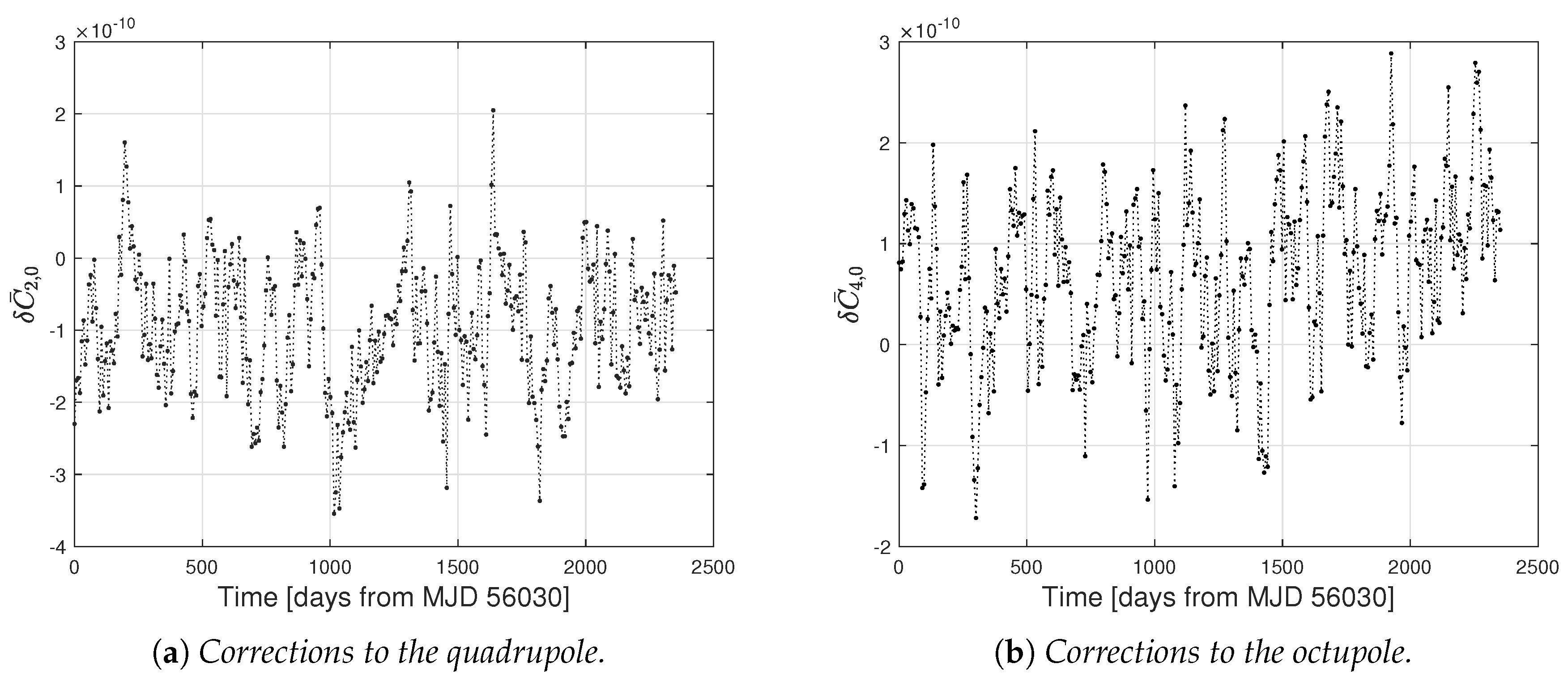
5
These are characterized by several periodic effects with, mainly, annual and inter-annual periodicities.
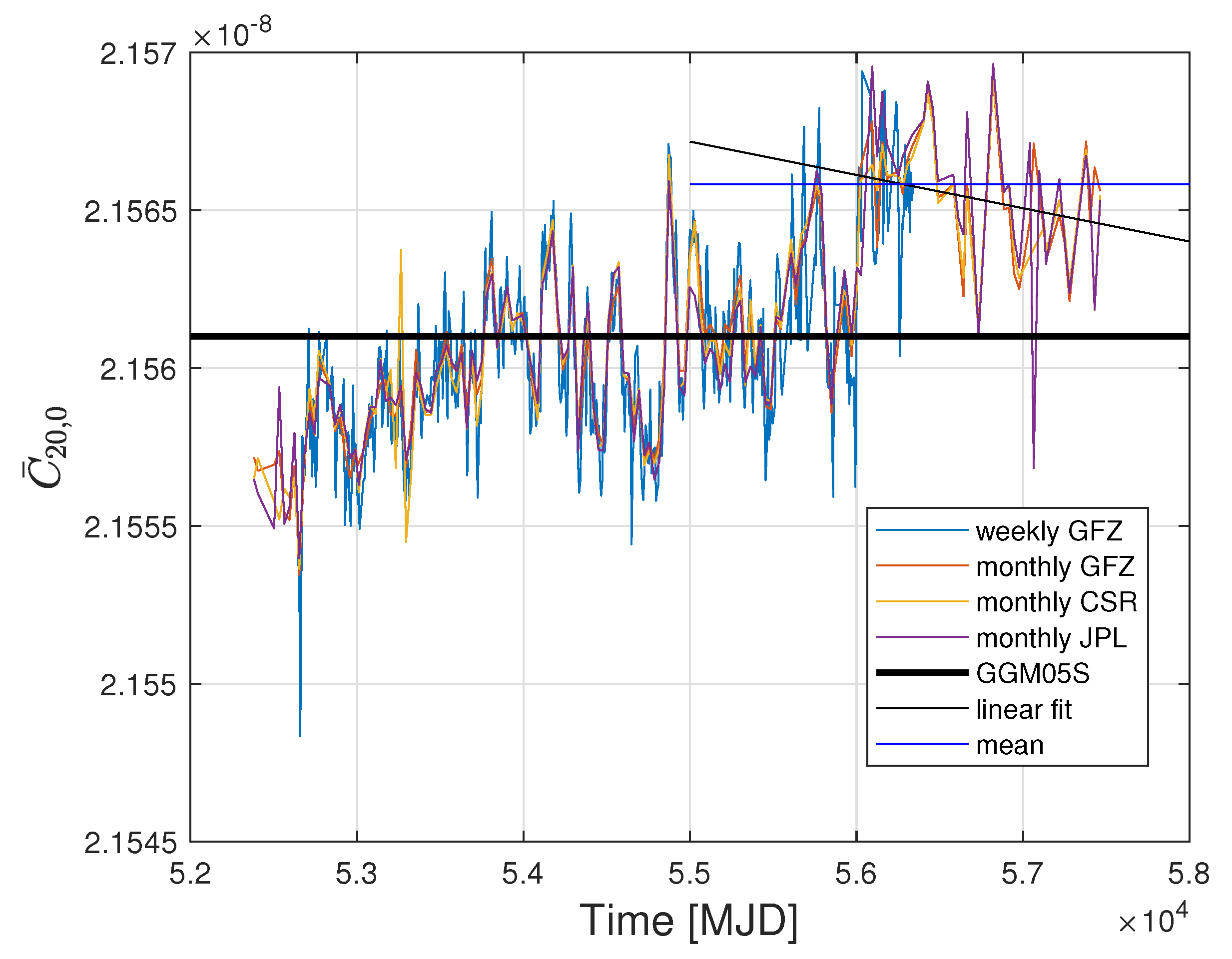
6
In [40], we linearly fitted the quadrupole coefficient that was obtained from GRACE monthly solutions and we used this fitted value in the data reduction of the satellites orbit. Furthermore, in that paper and for the GGM05S model, with regard to the Lense-Thirring effect measurement, we have also analyzed and compared the error related to the knowledge of the octupole coefficient with respect to the hexapole one, C ¯ 6 , 0 .
7
International Centre for Global Earth Models (ICGEM): Gravity Field Solutions for dedicated Time Periods: Release 05 and Release 06, http://icgem.gfz-potsdam.de/series. In the case of Release 06, no significant differences are present for the first 10 even zonal harmonics as compared to Release 05. Some small differences are present for the harmonics with degree 22 , but with no significant impact in the POD of the satellites.
8
Center for Space Research (CSR), University of Texas at Austin; GeoForschungsZentrum (GFZ), German Research Centre for Geosciences, Potsdam; Jet Propulsion Laboratory (JPL), California Institute of Technology, Pasadena.
9
The even zonal harmonics between degree = 22 and degree = 30 play a minor role, with no appreciable difference in the results. For the quadrupole coefficient, we also considered a more complete non-linear fit to the time behavior outlined by GRACE, with the inclusion of two periodic terms, one with a yearly frequency and one at twice this frequency. However, the final results have not shown a noticeable difference with respect to those obtained with a simpler linear fit.
10
Usually, these trends were those suggested by IERS Conventions [91], but were not always compatible with the results from GRACE monthly solutions. In the literature of the past measurements of the Lense-Thirring effect it has never been specified whether harmonics of degree higher than = 4 were modeled according to linear trends. Within the ILRS community, and since a few years, some harmonics are modeled up to degree 6 with secular trends, and very recently up to degree 12 in the case of the JCET Analysis Center.
11
For the same reason, we could not include the pericenter in our analysis. Our ongoing effort to improve the model for the thermal thrust perturbations [40,73,75,97] will hopefully allow us to include, in forthcoming measurements, also this element in the analysis, especially for LAGEOS II.
12
This is the solution currently used by the International Laser Ranging Service (ILRS) to realize the International Terrestrial Reference Frame (ITRF2014) [100], i.e., the practical realization of the International Terrestrial Reference System (ITRS) [91].
13
For the maximum degree of the field, we used an expansion up to degree and order 30 for the two LAGEOS and up to degree and order 90 for LARES, because of its smaller semi-major axis with respect to that of the two LAGEOS. In the case of LAGEOS satellites, the IERS Conventions [91] suggest at least an expansion up to degree and order 20. We have verified that for the two LAGEOS—considering an expansion up to degree and order 20, or 30, or 90—no significant difference in the POD of the satellites is produced.
14
From here on, when we refer generically to one of these solutions for the Earth’s gravitational field, we will always imply the modified solution for the first 10 even zonal harmonics, as described in the text.
15
More precisely, the solution of these equations for the combined RAAN of the three satelltes was explicitly computed in [48] following the original proposal of [108]. This approach was proposed, for the first time, by [109] in a Sun-planet context.
16
In this system of Equations we are neglecting the contributions from the mismodeling of the higher harmonics. Their contribution, however, is explicitly considered in the evaluation of the systematic errors, i.e., in the overall error budget of the measurement.
17
The orbital parameters are known with a very small relative uncertainty, such that the K coefficients can be considered, for our purposes, as error-free.
18
We directly provide the result for μ and not, as done in previous measurements of the Lense-Thirring effect, for the combined rate of the RAAN of the three satellites. This combination corresponds to a precession of 50.17 mas/yr.
19
We underline that the solution obtained for μ is independent of a possible imprint of the Lense-Thirring effect in the gravitational field coefficients. In fact, if this imprint were present, it would be mainly contained in the quadrupole coefficient, which is however eliminated by the combination that provides the Lense-Thirring parameter. However, from the tests we have performed in the past, there is no evidence of such a possibility.
20
In particular, the mismodeling of the gravitational perturbations, and the unmodeling of the thermal thrust effects in the case of the non-gravitational perturbations.
21
Where λ represents the ecliptic longitude of the Earth around the Sun.
22
We reiterate that the Lense-Thirring parameter μ obtained from the solution of the system of Equation (7) is independent of any static and dynamic error that characterizes the first two even zonal harmonics. The parameter μ obtained is however influenced by any error related to the even zonal harmonics with degree 6 . The correlations described in the text are strictly those between the relativistic parameter and the corrections to the first two even zonal harmonics with respect to their a priori values used in the POD.
23
This estimate was obtained applying the errors suggested by IERS Conventions (2010) to the amplitudes of the ocean tides of the GOT99.2 model. Anyway, in [71] we have shown that using more recent models for the ocean tides (as FES2004 and GOT4.7), the errors are of comparable magnitude with those of GOT99.2.
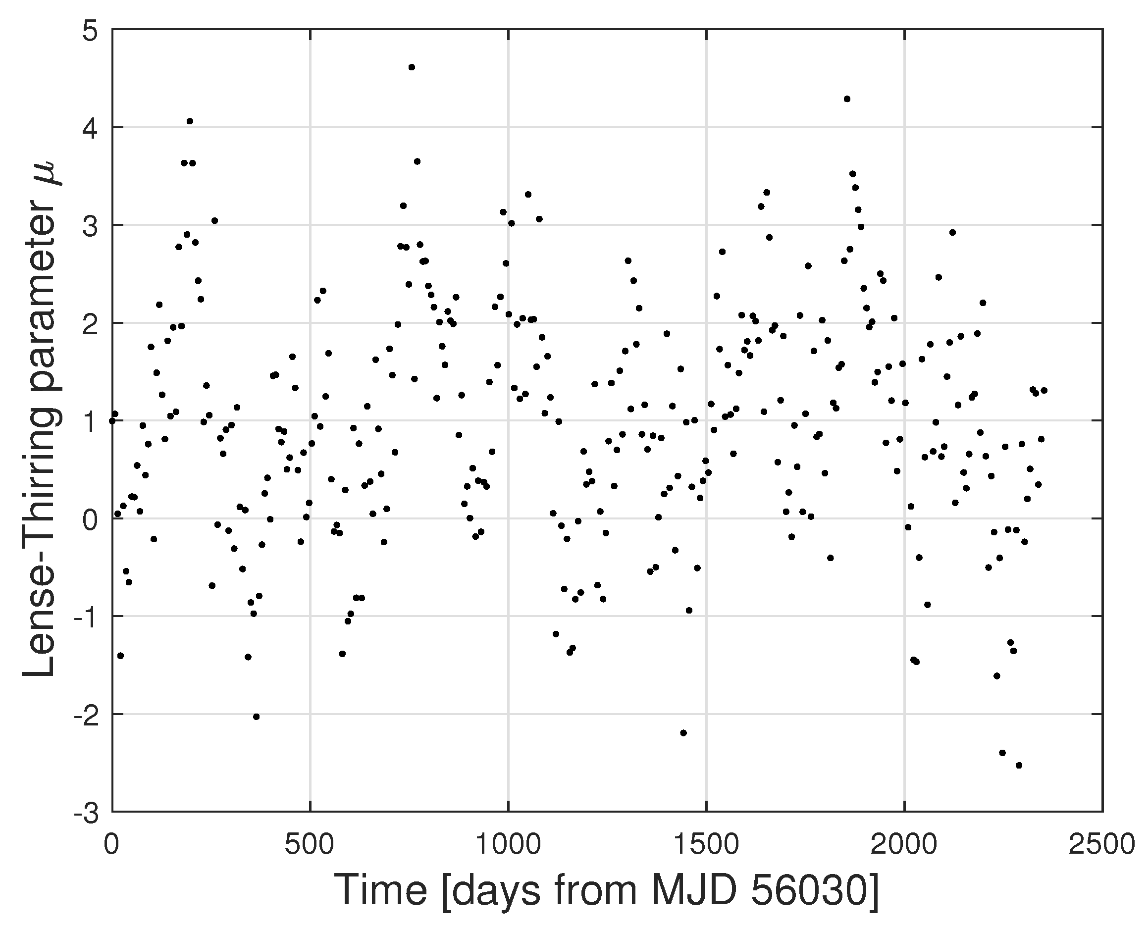
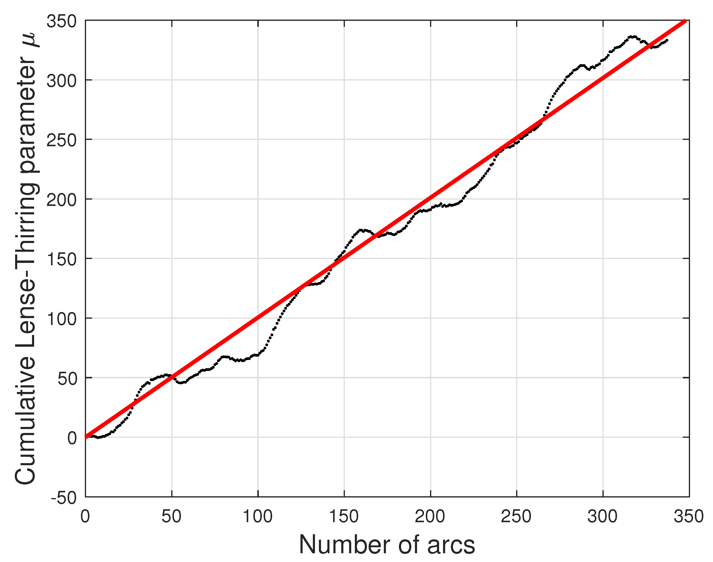
24
In this particular case, also the starting distribution was very close to a Gaussian one.
25
The ≈1% error for the periodic errors provided in Section 6 was obtained on the basis of a non-linear fit to the integrated residuals in the case of the GGM05S model.
Figure 1. Time behavior for the normalised C ¯ 20 , 0 coefficient. The horizontal axis is in Modified Julian Date (MJD). The measurements obtained for the coefficient from GRACE data by three independent Analysis Centers are compared with the static value provided by the GGM05S solution (heavy black line) and with the mean value (blue) and the linear behavior (soft black line) that we computed for this coefficient in the time span of our new analysis.
Universe 06 00139 g001
Figure 2. Corrections to the quadrupole ( C ¯ 2 , 0 ) and octupole ( C ¯ 4 , 0 ) coefficients estimated, arc by arc, on the time span of our analysis. The GGM05S model was considered for the background gravitational field of the Earth.
Universe 06 00139 g002
Figure 3. The Lense-Thirring parameter μ estimated, arc by arc, in the time span of our analysis. For the mean value we obtained μ = 0.99 ± 0.13 (at a 95% confidence level). The standard deviation of these residuals is about 1.20; this large value is due to the unmodeled periodic effects. The GGM05S model was considered for the background gravitational field of the Earth.
Universe 06 00139 g003
Figure 4. The Lense-Thirring parameter μ (black dots) obtained as the slope of the cumulative sum of the values shown in Figure 3. The horizontal axis shows the number of arcs of the satellites POD. The slope of the linear fit (red line) provides a value of μ = 1.0053 ± 0.0074 (at a 95% confidence level), see Table 4. The impact of the unmodeled periodic effects is reduced in the case of the cumulative residuals. The GGM05S model was considered for the background gravitational field of the Earth.
Universe 06 00139 g004
Figure 5. The estimated relativistic Lense-Thirring parameter μ as a function of the corrections simultaneously estimated for the quadrupole and octupole coefficients. The slightly negative correlation with the corrections to the octupole coefficient is however evident from the distribution of the values assumed by μ .
Universe 06 00139 g005
Figure 6. Comparison of the results obtained for the Lense-Thirring parameter μ from the solution of the system of Equation (7) for the four gravitational fields models considered in the present analyses. (a) The results for the mean value of μ is the same (after rounding) for the three models we considered in addition to GGM05S: μ = 0.98 ± 0.13 (at a 95% confidence level), again with a standard deviation of about 1.20. (b) The results for the slope obtained for the three additional models (EIGEN-GRACE02S, ITU_GRACE16 and Tonji-Grace02s) are shown in Table 4.
Universe 06 00139 g006
Figure 7. (a) Realizations for μ after 50,000 random permutations of the 337 residuals of Figure 3. (b) Distribution of the results for the Lense-Thirring parameter μ after the 50,000 permutations. For each realization, μ is obtained by means of the slope of the best linear fit like in Figure 4. The GGM05S model was considered as the background gravitational field of the Earth.
Universe 06 00139 g007
Figure 8. Distribution of the results for the Lense-Thirring parameter μ after 50,000 random permutations. The Gaussian fit for each of the gravitational fields considered in our analyses are shown.
Universe 06 00139 g008
Table 1. Mean orbital elements of the satellites.
ElementUnitSymbolLAGEOSLAGEOS IILARES
semi-major axis[km]a12,270.0012,162.077820.31
eccentricitye0.00440.01380.0012
inclination[deg]i109.8452.6669.49
Table 2. Rate, in millisecond of arc per year (mas/yr), for the secular Lense–Thirring precession on the right-ascension of the ascending node and on the argument of pericenter of LAGEOS, LAGEOS II, and LARES satellites.
Rate in the ElementLAGEOSLAGEOS IILARES
Ω ˙ LT +30.67+31.50+118.48
ω ˙ LT +31.23−57.31−334.68
Table 3. Correlations among the three estimated quantities evaluated as solutions of Equation (7) for the GGM05S model.
δ C ¯ 2 , 0 δ C ¯ 4 , 0 μ
δ C ¯ 2 , 0 +1.000+0.082+0.071
δ C ¯ 4 , 0 +1.000−0.179
μ +1.000
Table 4. Comparison of the results for the measurement of the relativistic Lense-Thirring precession among different models for the background gravitational field of the Earth, computed with the method of cumulative residuals. Errors appear to be equal due to rounding to the most significant digit. These results for the measured parameter μ are compatible (within their errors) with the prediction of GR for the Lense-Thirring precession: μ G R = 1 .
Model μ ± δ μ
GGM05S 1.0053 ± 0.0074
EIGEN-GRACE02S 1.0002 ± 0.0074
ITU_GRACE16 0.9996 ± 0.0074
Tonji-Grace02s 1.0008 ± 0.0074
Table 5. Results for the Lense-Thirring parameter after the Gaussian fit described in the text and based on 50,000 random permutations of the residuals obtained for each 7-day arc from the POD described in Section 6. The error σ μ represents the standard deviation of each Gaussian fit at a 95% confidence level.
Model μ ¯ ± σ μ
GGM05S 0.9889 ± 0.0294
EIGEN-GRACE02S 0.9778 ± 0.0292
ITU_GRACE16 0.9772 ± 0.0291
Tonji-Grace02s 0.9788 ± 0.0292

