the Creative Commons Attribution 4.0 License.
the Creative Commons Attribution 4.0 License.
 | 28 Aug 2020
Distribution of planktonic foraminifera in the subtropical South Atlantic: depth hierarchy of controlling factors
Raphaël Morard
Lukas Jonkers
Igor M. Venancio
Runa Reuter
Adrian Baumeister
Ana Luiza Albuquerque
Michal Kucera
Temperature appears to be the best predictor of species composition of planktonic foraminifera communities, making it possible to use their fossil assemblages to reconstruct sea surface temperature (SST) variation in the past. However, the role of other environmental factors potentially modulating the spatial and vertical distribution of planktonic foraminifera species is poorly understood. This is especially relevant for environmental factors affecting the subsurface habitat. If such factors play a role, changes in the abundance of subsurface-dwelling species may not solely reflect SST variation. In order to constrain the effect of subsurface parameters on species composition, we here characterize the vertical distribution of living planktonic foraminifera community across an east–west transect through the subtropical South Atlantic Ocean, where SST variability was small, but the subsurface water mass structure changed dramatically. Four planktonic foraminifera communities could be identified across the top 700 m of the transect. Gyre and Agulhas Leakage surface faunas were predominantly composed of Globigerinoides ruber, Globigerinoides tenellus, Trilobatus sacculifer, Globoturborotalita rubescens, Globigerinella calida, Tenuitella iota, and Globigerinita glutinata, and these only differed in terms of relative abundances (community composition). Upwelling fauna was dominated by Neogloboquadrina pachyderma, Neogloboquadrina incompta, Globorotalia crassaformis, and Globorotalia inflata. Thermocline fauna was dominated by Tenuitella fleisheri, Globorotalia truncatulinoides, and Globorotalia scitula in the west and by G. scitula only in the east. The largest part of the standing stock was consistently found in the surface layer, but SST was not the main predictor of species composition either for the depth-integrated fauna across the stations or at individual depth layers. Instead, we identified a pattern of vertical stacking of different parameters controlling species composition, reflecting different aspects of the pelagic habitat. Whereas productivity appears to dominate in the mixed layer (0–60 m), physical properties (temperature, salinity) become important at intermediate depths and in the subsurface, a complex combination of factors including oxygen concentration is required to explain the assemblage composition. These results indicate that the seemingly straightforward relationship between assemblage composition and SST in sedimentary assemblages reflects vertically and seasonally integrated processes that are only indirectly linked to SST. It also implies that fossil assemblages of planktonic foraminifera should also contain a signature of subsurface processes, which could be used for paleoceanographic reconstructions.
- Article
(24285 KB) -
Supplement
(2502 KB) - BibTeX
- EndNote


The composition of planktonic foraminifera communities in the water column changes in response to key properties of their habitat such as water temperature, salinity, and food availability (Bé, 1977; Ottens, 1992; Ufkes et al., 1998; Schiebel and Hemleben, 2017). In contrast, the composition of sedimentary assemblages, integrating the seasonal shell flux across years to centuries consistently appears to be best predicted by temperature alone (Morey et al, 2005), and this relationship has been exploited by paleoceanographers to reconstruct past temperature (e.g., Kucera et al., 2005). However, the reason for the strong relationship of temperature with sedimentary assemblage composition remains poorly understood, especially in the light of species composition data derived from the plankton (Jentzen et al., 2018). If species composition primarily reflects other factors and the covariance of these factors with temperature differed in the past, then the variability of fossil assemblages may not solely reflect temperature variation, violating a key assumption of the transfer function methods used to convert past assemblage composition to temperature (Telford and Birks, 2005; Juggins et al, 2015). Indeed, data from plankton tows and sediment traps show that the living community likely responds to multiple processes in the water column (Ortiz et al, 1995; Schiebel et al, 2001; Field et al, 2006; Storz et al, 2009; Jonkers and Kucera, 2015). This does not mean that the planktonic foraminifera community does not respond to temperature, but it implies that this relationship may be indirect, mediated by temperature control on productivity or other aspects of the foraminifera habitat. The lack of understanding on how exactly the environment shapes planktonic foraminifera communities is a common issue for the choice of variables used to construct forward models (Žarić et al, 2005; Lombard et al, 2009; Fraile et al, 2009; Kretschmer et al, 2016), as well as transfer function models (e.g., Morey et al, 2005; Siccha et al, 2009; Telford et al., 2013).
Attempts to disentangle the processes that affect planktonic foraminifera community composition must consider the vertical dimension of species habitat. Observations from vertically resolved plankton nets indicate a vertical range of the living community up to 1000 m with the majority of the standing stock concentrated in the upper 300 m (Bé, 1960; Schiebel, 2002). Because their habitat stretches across such a large depth range, communities at different depths should reflect vertically differentiated controlling processes: light intensity and photosynthesis are only relevant in the photic zone, whereas at depth, processes regulating the export of organic matter from the surface layer may control the food that is available to the community. It is therefore likely that there will not be a universal predictor of community composition across the depth range of their habitat. Instead, we hypothesize that the community will reflect an integrated signal of depth-stratified processes affecting composition in different depth layers.
Planktonic foraminifera counts from stratified plankton net samples coupled with observations of physical and chemical parameters in the water column provide the most direct means to resolve whether or not such a depth hierarchy of controlling factors exists. Unfortunately, most previous studies based on foraminifera census counts from plankton nets do not present direct measurements of environmental parameters such as temperature, salinity, chlorophyll a, and dissolved oxygen (DO); lack an appropriate depth resolution that comprise the all or most of species found in sediment assemblages; or originate from regions where surface and subsurface properties are highly correlated (Bé, 1960; Ottens, 1992; Kemle-von Mücke and Oberhänsli et al., 1999; Lončarić, 2006; Sousa et al., 2014; Rebotim et al., 2017). In this study, we analyze stratified plankton net samples collected in the subtropical South Atlantic, along a transect covering the gradient from productive coastal waters off South Africa to the oligotrophic waters of the subtropical gyre off Brazil. The transect has been chosen because it samples a region where sea surface temperature (SST) variability is small but the subsurface water mass structure differs drastically. We make use of the availability of in situ vertically resolved measurements of environmental parameters and aim to determine which processes explain compositional variability at different depth layers across the transect.
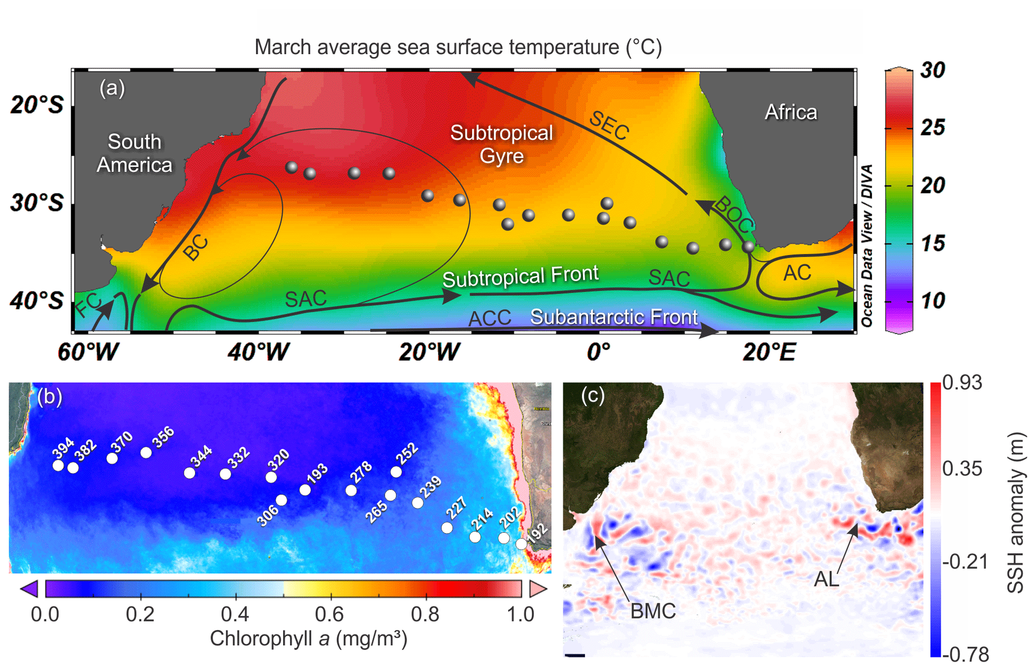
Figure 1Map of the South Atlantic Ocean showing the locations of the stations of the M124 cruise. (a) March sea surface temperature (SST) from World Ocean Atlas 2013 and the main surface current systems (modified from World Ocean Atlas 2013 and Stramma and England, 1999). (b) Average 2002–2018 surface chlorophyll a measured by satellite from MODIS – AQUA. (c) Sea surface height anomaly above the sea level on 1 March 2016 (sampling of station 202) from Ssalto/Duacs (SAC – South Atlantic Current; ACC – Antarctic Circumpolar Current; SEC – South Equatorial Current; BOC – Benguela Oceanic Current; AC – Agulhas Current; BC – Brazil Current; MC – Malvinas Current; AL – Agulhas Leakage; BMC – Brazil – Malvinas Confluence zone).
The M124 cruise (Karstensen et al., 2016) took place between 29 February to 16 March 2016 on board the RV Meteor, sampling across the subtropical South Atlantic (26–34∘ S, 18∘ E to 36∘ W) along an east–west (zonal) transect (Fig. 1a). Planktonic foraminifera were collected at 17 stations using a Multiple Plankton Sampler (MPS, HydroBios, Kiel) with 50×50 cm opening, 100 µm mesh size, and five sampling nets. Two MPS casts were performed per station to resolve the planktonic foraminifera standing stock in nine depth levels (700–500, 400–300, 300–200, 200–100, 100–80, 80–60, 60–40, 40–20, 20–0 m) with the exception of the two easternmost stations (192 and 202), where the maximum sampling depth was 100 and 500 m, respectively (Table 1).
Table 1Stations of the M124 cruise, location, time (day/month/year), environmental parameters for the mixed and permanent thermocline (250 m) layers, depth intervals, method used for preservation of the sample, counting size, and filtered seawater volume.
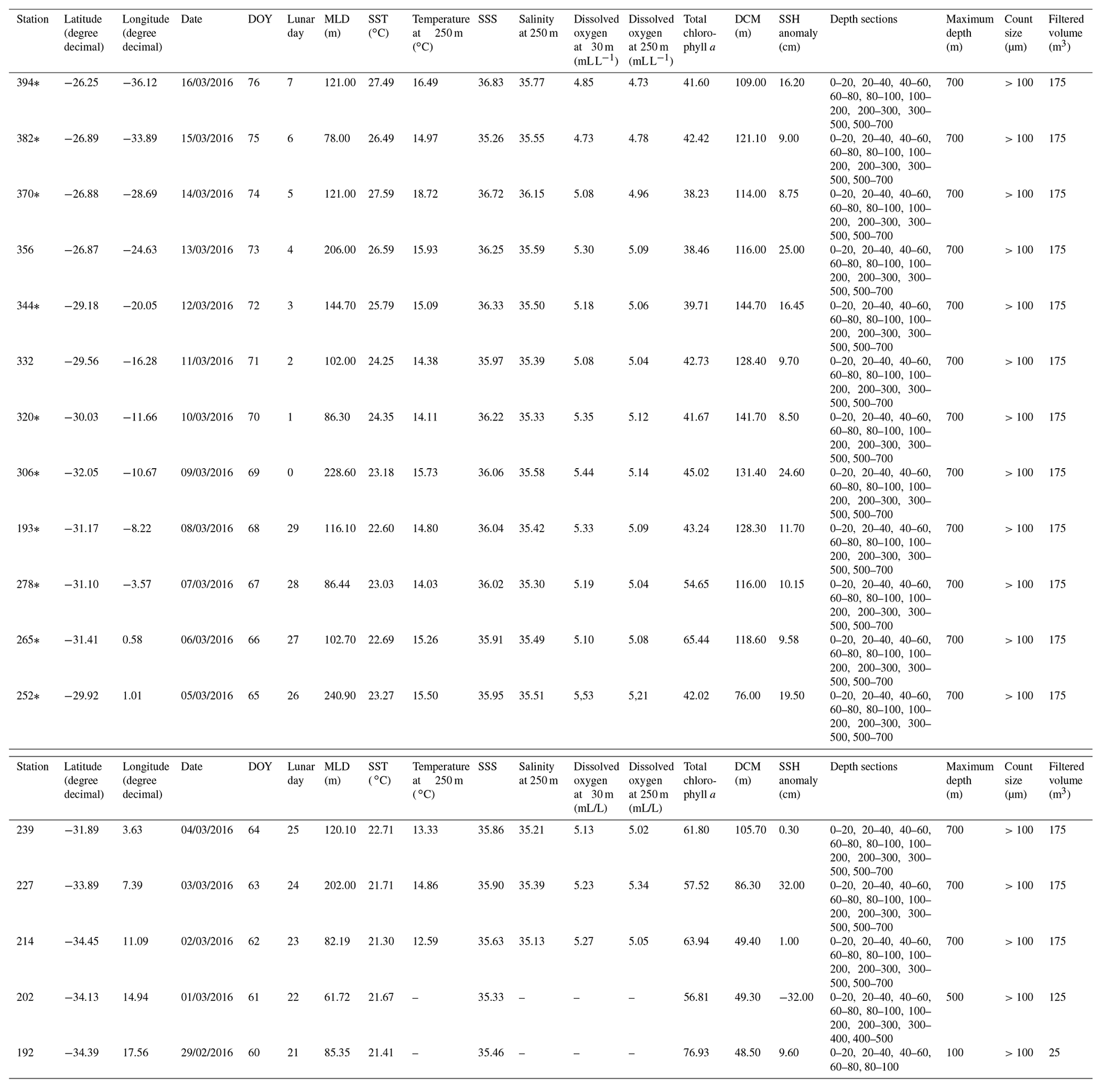
*Dissolved oxygen measurements were obtained by interpolation or DO measurements from the nearest stations (see Karstensen et al., 2016)
The MPS was equipped with a Sea & Sun Conductivity–Temperature–Depth (CTD) instrument providing in situ measurements of temperature, salinity, and chlorophyll a concentration. Dissolved oxygen (DO) content was measured during separate CTD casts using a Seabird Electronics sensor mounted on the rosette. The sensor was calibrated on board through comparison with oxygen concentrations determined by titration (Karstensen et al., 2016). Concentration data were averaged for the plankton net intervals and in cases where a plankton haul was not accompanied by a CTD cast (Table 1); values were linearly interpolated along longitude. For the westernmost multi-net we used DO data from the nearest CTD cast. Due to a sensor failure DO data are not available for stations 192 and 202. To assess the influence of eddies (a prominent feature of South Atlantic oceanography, Stramma and England, 1999) on the planktonic foraminifera distribution, sea surface height data were obtained from SSALTO/DUACS for each station at the day of sampling.
All planktonic foraminifera specimens were picked onboard and dried on micropaleontological slides and frozen, with the exception of the station 192. At this station, the samples were partly picked, and the remaining plankton samples were frozen in a sampling bag and further processed on shore. All samples were shipped frozen to Bremen University (Germany). A detailed description of the planktonic foraminifera sampling process is given in Karstensen et al. (2016). Planktonic foraminifera were counted and identified to species level following Schiebel and Hemleben (2017). Descriptions and images of the most abundant species can be found in Appendix A and Plates A1–A5. Specimens with cytoplasm in the last whorl were considered as living, whereas tests with no (or almost no) visible cytoplasm in the last whorl, displaying a distinctive white coloration of the test, were considered dead. This distinction is likely overestimating the number of living specimens because the presence of cytoplasm itself does not guarantee that a specimen was alive during collection. It results in a slightly deeper estimate of the living depth, caused by dead specimens with cytoplasm being found beneath their original habitat (see Rebotim et al, 2017). In addition, specimens that showed adult morphology were separated from preadult ontogenetic stages. The ontogenetic classification of specimens followed the morphological differences between preadult and adult stages as summarized by Brummer et al (1986). Species with small morphological differences among the ontogenetic stages (e.g., Globigerinella calida, Globigerina bulloides, Globorotalia scitula, and Globorotalia truncatulinoides) were classified as “preadult” when they lacked morphological features that define the neanic to adult stage transition as proposed by Brummer et al (1986). In many small-sized species (e.g., Tenuitella fleisheri, Turborotalita clarkei, Turborotalita quinqueloba, Globigerinita glutinata, and Globigerinoides tenellus), preadults could not be identified due to the high morphological similarity among those that were grouped together in the category “unidentified juveniles”. Initial ontogenetic stages of Globigerinoides ruber white and Globigerinoides elongatus were lumped together as “G. ruber juveniles” because the diagnostic trait of the two species is only observed among adult specimens. Species counts were converted to concentrations using the volume estimated from the thickness of the collection interval. The concentrations of living specimens were subsequently used to calculate average living depth (ALD) and vertical dispersion (VD) following Rebotim et al. (2017).
Multivariate analyses were used to identify covarying species (faunas) and to assess which of the tested environmental variables determine the spatial and vertical distribution of individual species and species communities. Covarying species (faunas) were identified by cluster analysis using relative abundance of species in each depth level, allowing a joint vertical and zonal analysis across the transect. The analysis was carried out using Bray–Curtis distance and the unweighted pair-group method with arithmetic mean algorithm. The relationship between species concentrations and environmental parameters was determined by ordination analysis. We chose the canonical correspondence analysis (CCA) as the gradient length indicated that methods for unimodal distribution are more appropriate (Legendre and Gallagher, 2001). The spatial distribution of the planktonic foraminifera communities across stations was tested against SST and SSS at the surface (accounting for conditions affecting most of the fauna at each station) and subsurface (250 m, accounting for conditions affecting the subsurface component of the fauna), SSH and mixed-layer depth (accounting for the vertical structure of the water column) and chlorophyll a (accounting for the overall productivity regime at each station). Then the species concentrations at each station were tested separately for each of the nine depth layers against in situ SST, SSS, chlorophyll a, and DO, always taking parameter values at the center of each depth interval. This analysis excluded the two shallower easternmost stations. Cluster analysis was carried out using the Past software (versions 3.16) (Hammer et al., 2001) and CCA analysis were carried out using in R Core team (2019) using the vegan package (Oksanen et al., 2019).
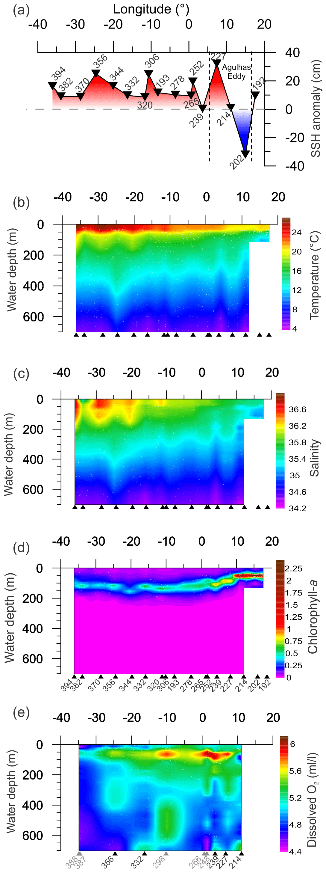
Figure 2Variation measured in environmental parameters from CTD and satellite for the upper 700 m of the water column along the transect. Triangles indicate the location of sampling sites (black triangles are sites with multi-net casts, gray triangles are sites without multi-net casts from Karstensen et al, 2016, used for DO gridding). Panels (a)–(c) show gridded values of CTD measured parameters. (d) Satellite sea surface height from SSALTO/DUACS for the respective stations sampling days. (e) Dissolved oxygen, the gridding used some stations near to stations with multi-net cast (grey numbers), as no oxygen data are available (see Table 1 for details).
The studied region comprises three main oceanographic systems: the Subtropical Gyre (west and east), the Agulhas Leakage, and the Benguela Current (Fig. 1). The western Subtropical Gyre (36–16∘ W) is characterized by high temperature and salinity and low nutrient concentrations. Recirculation of warm waters from the Brazil and South Atlantic currents occurs in the western Subtropical Gyre and leads to the accumulation of warm and saline waters resulting in a thick and warm mixed layer (Peterson and Stramma, 1991). In contrast, the mixed layer in the eastern Subtropical Gyre (16∘ W–5∘ E) is colder. The Agulhas Leakage sector (5–15∘ E) is characterized by the occurrence of large eddies formed by the interaction between waters from the Agulhas system and waters of the Subtropical Gyre sector (Stramma and England, 1999), which is indicated by larger SSH anomalies between stations 227 and 202 (7–15∘ E, Figs. 1c, 2a). Tongues of nutrient-rich waters from the Benguela upwelling system are entrained in westward-moving eddies, causing elevated productivity far offshore in the Agulhas Leakage (Fig. 1b). Finally, the Benguela Current (17∘ E) differs from the other systems by its low temperature, salinity, and high productivity due to the Benguela coastal upwelling. It receives a contribution of warm waters from the Agulhas Leakage and cold waters from penetrations of the Subtropical Front (Peterson and Stramma, 1991; Fig. 1c).
The upper 700 m of the South Atlantic comprises three water masses. The first 100–200 m of the water column in the Subtropical Gyre is composed of the Tropical Water (TW) (Stramma and England, 1999). South Atlantic Central Water (SACW) is found in the permanent thermocline (6–20 ∘C isotherm) and halocline (34.3–36.0) (Stramma and England, 1999), and its upwelling is responsible for high productivity off Southwest Africa. Antarctic Intermediate Water (AAIW) can be observed below the permanent thermocline. It has low temperature and salinity but high nutrient and oxygen concentrations (Stramma and England, 1999). Salinity above 36 and high surface temperatures (Fig. 2b and c) indicated the presence of the Tropical Water (TW) that occupied the upper 200 m between stations 394 and 344 (36–20∘ W) and the upper 50 m between the stations 332 and 252 (16∘ W–1∘ E). Salinity below 36 and low oxygen concentrations indicate the influence of SACW (Fig. 2c and e), which is particularly thick in the center of the transect (16∘ W–1∘ E). Between stations 239 and 192 (3–17∘ E) low salinity and low temperature (Fig. 2b and c) indicates a near surface presence of SACW, which is mixing with warm surface waters from the Agulhas Leakage. The AAIW was identified by high oxygen concentration (Fig. 2e) and salinity values up to 34.3 that are viewed only in the deepest layers (near to 700 m) at stations 214 and 239. In the other stations, the SACW was present down to 700 m.
The thermally stable upper mixed layer (UML) occupied the first 30–40 m of the water column at all stations (Fig. 2b). The UML temperature was higher in the western Subtropical Gyre, gradually decreasing towards the east. Below the UML, referred here as lower mixed layer (LML), a sharp temperature decrease is observed until about 100 m, followed by near constant values until about 200 m, and a slow temperature decrease afterwards. Since the expedition took place during the late summer, the 40–100 m sharp decrease of temperature likely represents the seasonal thermocline, and the beginning of the permanent thermocline layer was therefore defined where the low gradual temperature decline starts. At stations where the temperature decrease started just below the seasonal thermocline, the boundary between the LML and permanent thermocline was placed below the seasonal thermocline. The delimitation of mixed layer and permanent thermocline boundaries across the studied transect is shown in Fig. S1.
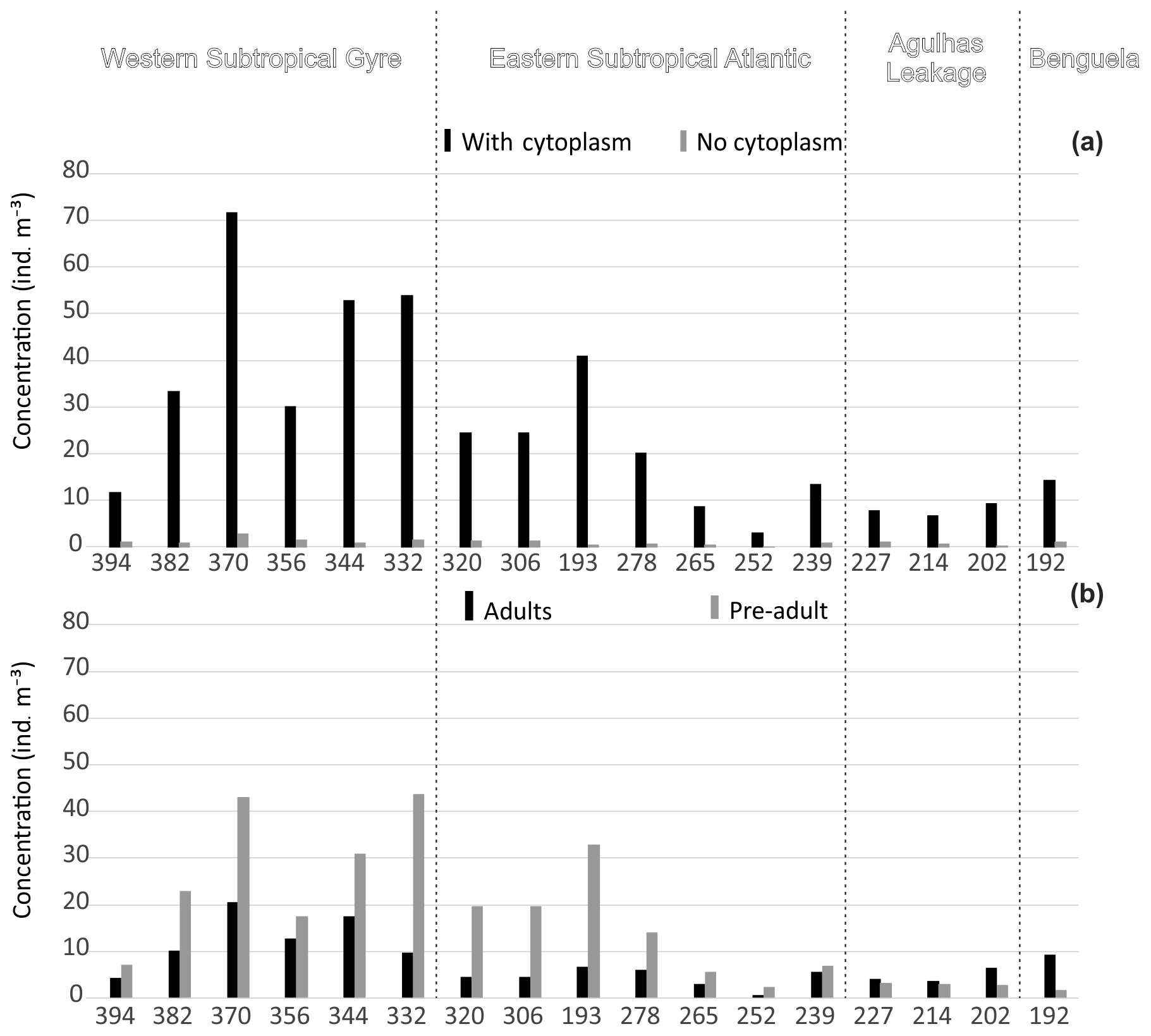
Figure 3Concentration of planktonic foraminifera in the upper 100 m. (a) Total concentration separated by presence of cytoplasm (living and dead). (b) Total standing stock separated by ontogenetic stage. Refer to the Supplement (Figs. S2 and S3) for the entire profile.
The salinity maximum was found at the surface, except in the western Subtropical Gyre, where it occurred between 50 and 100 m, and permanent halocline coincided with the permanent thermocline at around 200 m. The DO content varied between 4.5 and 6 mL L−1 with high concentrations at LML and low values below 300 m. The DO content in the surface mixed layer was higher at the eastern Subtropical Gyre than in the western Subtropical Gyre (Fig. 1e). At the permanent thermocline, DO content was generally low with lowest values occurring in a broad area of the western Subtropical Gyre where values below 5.0 mL L−1 can be seen up to 150 m. The central Subtropical Gyre around 10∘ W is marked by oxygen concentrations above 5.7 mL L−1. Towards the eastern Subtropical Gyre, oxygen concentrations decrease, but remain higher and more variable than in the west.
The highest chlorophyll a concentrations (63–77 µg L−1) occurred between stations 214 and 192 (11–17∘ E) with the Deep Chlorophyll Maximum (DCM) at about 50 m (Fig. 2d). Moderate chlorophyll a concentrations (55–65 µg L−1) and a DCM between 50 and 100 m were seen at stations 265, 239, and 227 (3–7∘ E). The other stations had lower values ranging from 38 to 45 µg L−1 and a DCM below 100 m. High chlorophyll a values in the east are associated with the Benguela upwelling system (station 192) and its tongues that mix with oligotrophic waters of Agulhas Leakage (stations 214 and 202). Low chlorophyll a concentrations in the western and central South Atlantic are associated with strong stratification of the Subtropical Gyre.

Figure 4Variation of the depth habitat and standing stock (integrated over the upper 550 m) of main species across the subtropical South Atlantic. Species data are compared with temperature (in ∘C) (color filling). Chlorophyll a is shown with thin lines delimiting layers with 0.2 mg m−3 and a thick line indicating the chlorophyll a apex. Sea surface height (SSH) and boundaries of surface mixed layer and mixed and permanent thermocline layers are shown as continuous white lines. Note that the panels have varying depth scales.
4.1 Concentration and distribution of living and dead planktonic foraminifera
We identified 38 species of planktonic foraminifera of which 22 yielded five or more individuals per station, allowing an the analysis of their habitat depth and zonal variation (Table 2, Appendix A, Plates A1–A5). We observed high standing stocks of Globigerinoides ruber (pink and white), Globigerinoides elongatus, Trilobatus sacculifer, Globoturborotalita rubescens, Globigerinoides tenellus, Tenuitella iota, and Globigerinita glutinata in the mixed layer of the Subtropical Gyre and Agulhas Leakage region. In the Benguela Current and the subsurface sector of the Agulhas Leakage area, we observed high abundances of Neogloboquadrina dutertrei, Neogloboquadrina pachyderma, Neogloboquadrina incompta, rounded specimens of Globorotalia crassaformis, and Globorotalia inflata. The water column below 100 m (permanent thermocline layer) across the whole transect had high abundances of Tenuitella fleisheri, Globorotalia truncatulinoides (left coiling), Globorotalia scitula and Hastigerina pelagica. Apart from the Benguela and permanent thermocline-dwelling species, some other species also had restricted distributions. G. ruber pink was found only in the western Subtropical Gyre, Candeina nitida occurred from station 356 (western Subtropical Gyre) to 265 (eastern Subtropical Gyre), Globorotalia menardii occurred in high abundances in the first 100 m at three western stations (394, 382 and 370), and conical specimens of G. crassaformis were observed rarely in the permanent thermocline of the western Subtropical Gyre.

Figure 5Average living depth (ALD) and vertical dispersion (VD) of the most abundant planktonic foraminifera species sorted by depth (in base 2 logarithmic scale) with the defined depth groups.
Concentrations of planktonic foraminifera increased from around 10 shells m−3 in the east to a maximum of 75 shells m−3 in the central part of the western Subtropical Gyre (Fig. 3a). Concentrations of living specimens were always higher in the upper 100 m of the water column (Fig. S2), with a gradual increase in the proportion of dead specimens below 100 m and almost no living specimens occurring below 500 m. The lowest concentrations (living and dead specimens) were observed in the deepest sections of stations 394, 370, and 227. Preadult specimens were abundant in central gyre stations (Fig. 3), where station 306 (11∘ W) had almost 100 % preadult specimens in the upper 40 m (Fig. S3). The number of adults tended to increase with depth (>40 m depths) with preadults being virtually absent below 100 m. The exception was Globorotalia crassaformis in the eastern stations. The concentrations of living adults were higher than those of living preadults (near 100 % adult) at stations 214 and 192, where most of the fauna consisted of N. pachyderma, N. incompta, G. inflata, and G. crassaformis.
Table 2Average living depth and vertical dispersion of the 30 species with at least two living individuals counted in a station. The list was sorted by the maximum number of occurrences of living individuals within the samples. Interpretations of depth habitat and its corresponding variability or stability were performed for species with enough number of individuals. Species with * had an insufficient number of living individuals or the population was dominated by preadults, rendering interpretations about the depth habitat doubtful.
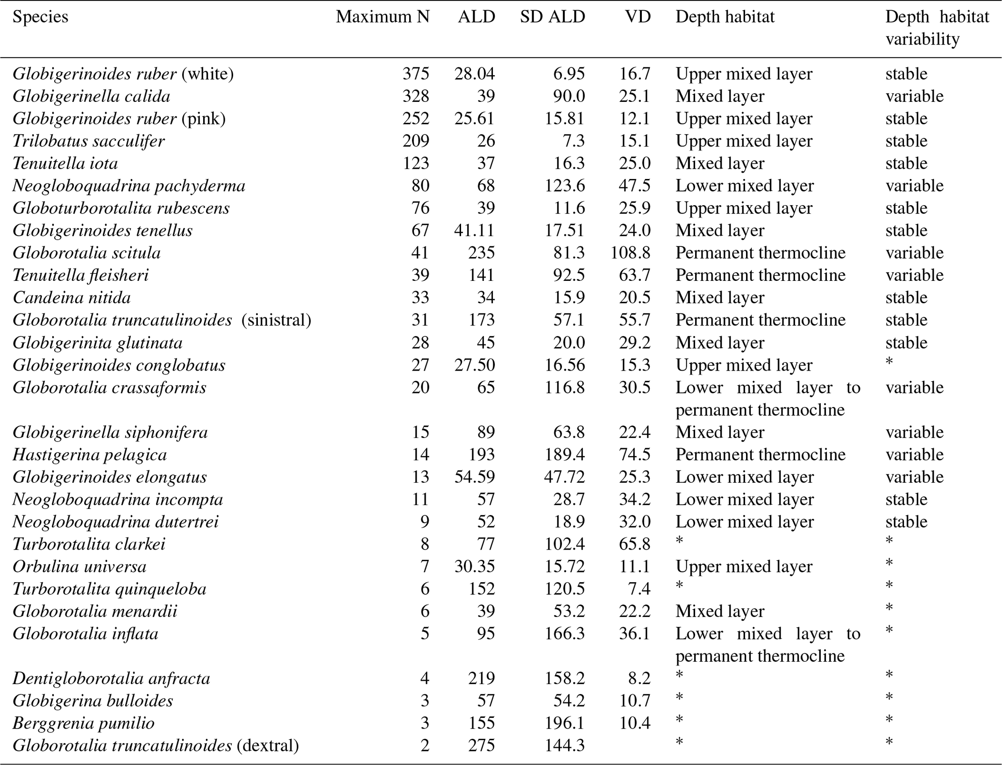
The species G. ruber (pink and white), T. sacculifer, Orbulina universa, and Globigerinoides conglobatus had an ALD between 20 and 30 m with a VD up to 16 m with little zonal variation (Figs. 4, 5). G. ruber white and T. sacculifer were present at all stations; the other two species were only found on the western side of the Subtropical Gyre, where temperature and salinity values were high. Most of the specimens of G. conglobatus were preadult. The ALDs of C. nitida, G. rubescens, T. iota, G. menardii, G. calida, G. tenellus, and G. glutinata were between 30 and 40 m and the VD was between 20 and 30 m (Fig. 5). We observed more zonal variation in both ALD and VD for these species. Most of the G. calida individuals found at stations 332 and 320 were preadult and they inhabited the upper 40 m, contrasting with others stations where the ALD varied between 40 and 70 m (Fig. 4). Specimens of G. menardii were identified in stations of the western Subtropical Gyre and the Agulhas Leakage area, but the low abundance in the latter area did not allow reliable ALD and VD estimates. The species C. nitida was most abundant in the eastern Subtropical Gyre stations (station 320–265), whereas G. rubescens, G. tenellus, T. iota, and G. glutinata were found in similar abundances along the entire transect (Fig. 4).
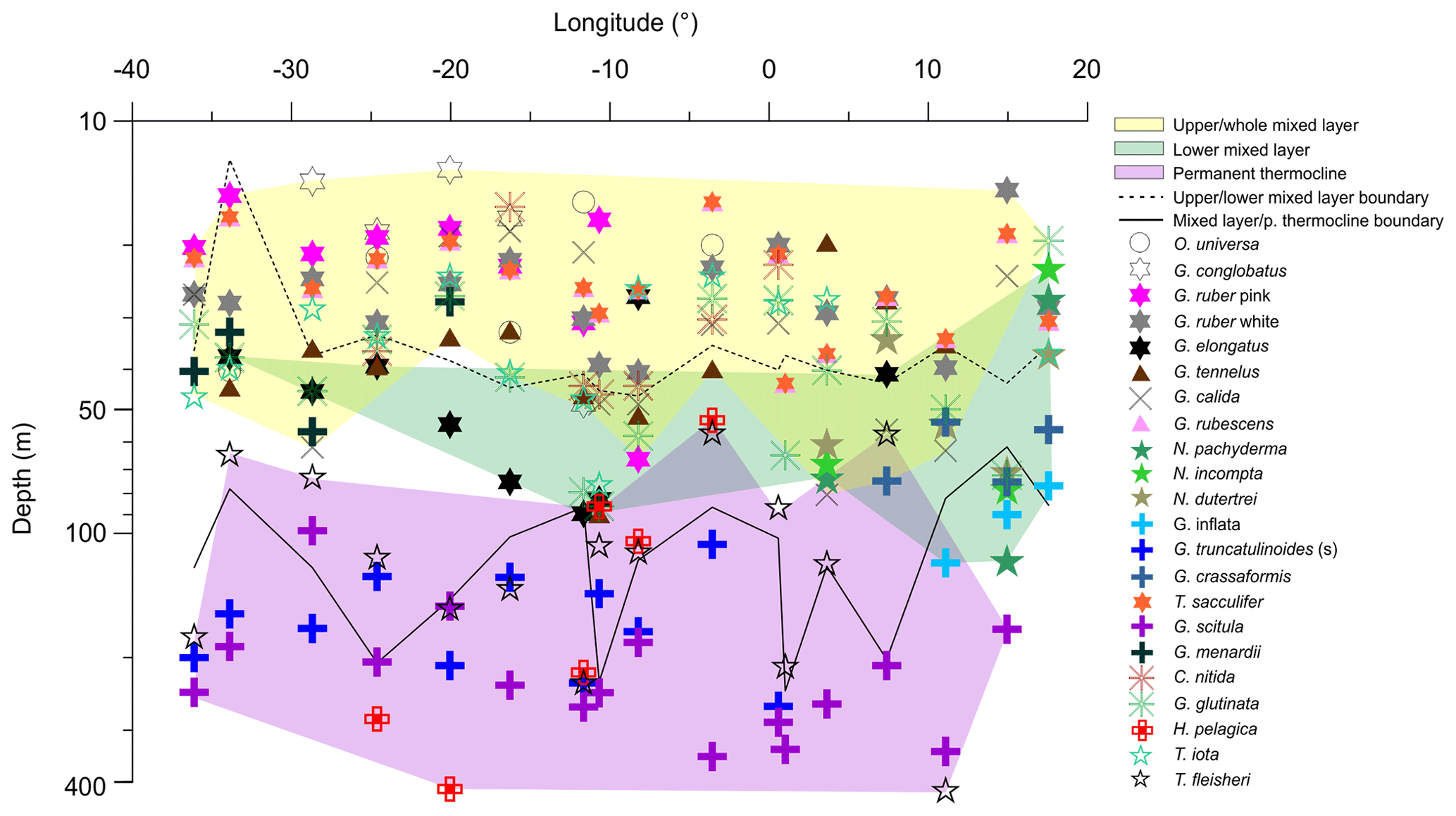
Figure 6Average living depth (ALD) of the most abundant species along the transect in the South Atlantic. Depth groups are highlighted by different color filling. Note the ALD separation above and beneath 100 m and the lower mixed layer group that is more obvious on the eastern side.

Figure 7(a) Cluster analysis of relative community composition in all stations and depths sections. (b) Graphical representation of clustered groups along the whole transect. Samples without living specimens are highlighted with an “x”. (c) Zonally and vertically interpreted communities across the subtropical South Atlantic. Station names were placed with warm to cold colors in (a) and (b) in order to separate and locate different depth layers. The main species contribution for each group is shown in Table 3.
The ALD of G. elongatus, G. crassaformis, N. dutertrei, N. incompta, and N. pachyderma was between 50 and 70 m with a VD between 25 and 50 m (Table 2, Fig. 4). This depth range corresponds to the seasonal thermocline. Specimens of G. elongatus occurred at higher abundances in the western Subtropical Gyre and at stations 320 and 306 of the eastern Subtropical Gyre, where their ALD was largest (between 80 and 90 m, Fig. 4). The remaining four species were more abundant in the Benguela Current and seasonal thermocline of the Agulhas Leakage. However, specimens of G. crassaformis found on the eastern side of the transect were usually preadult and morphologically similar to Globorotalia inflata (see Appendix A and Plate A3). Typical adult specimens (see Appendix A and Plate A4) were found in the permanent thermocline layer in the western Subtropical Gyre at insufficient abundance to calculate a reliable ALD.
The ALD of Tenuitella fleisheri, Hastigerina pelagica, Globorotalia inflata, Globorotalia truncatulinoides, and Globorotalia scitula ranged between 95 and 250 m with VDs between 36 and 110 m (Table 2, Fig. 4). Specimens of G. inflata were present in small numbers only in the seasonal and permanent thermocline layer of stations 192, 202, and 214 (Benguela and Agulhas Leakage). Specimens of H. pelagica were encountered below 200 m in the entire Subtropical Gyre and large living specimens were also present in the surface layer of station 278 (eastern Subtropical Gyre). However, the number of empty tests was usually high for this species, and only five stations had enough numbers of living specimens to calculate a reliable ALD. Specimens of G. truncatulinoides were most abundant inside the Subtropical Gyre (stations 394–265) and were usually sinistral. Dextral coiling G. truncatulinoides were very rare, which did not allow distinguishing the ALDs of the two coiling variants. T. fleisheri and G. scitula were abundant at most stations, but the highest concentrations tended to differ zonally and vertically. Specimens of T. fleisheri were more abundant between 100 and 300 m in the western Subtropical Gyre. Specimens of G. scitula were more abundant in the eastern Subtropical Gyre and Agulhas Leakage, with ALD usually below 200 m. At stations under influence of Benguela upwelling (stations 202 and 192), G. scitula and other permanent thermocline-dwelling species were encountered in shallower waters, but for T. fleisheri and G. truncatulinoides the number of individuals was insufficient to estimate ALD.
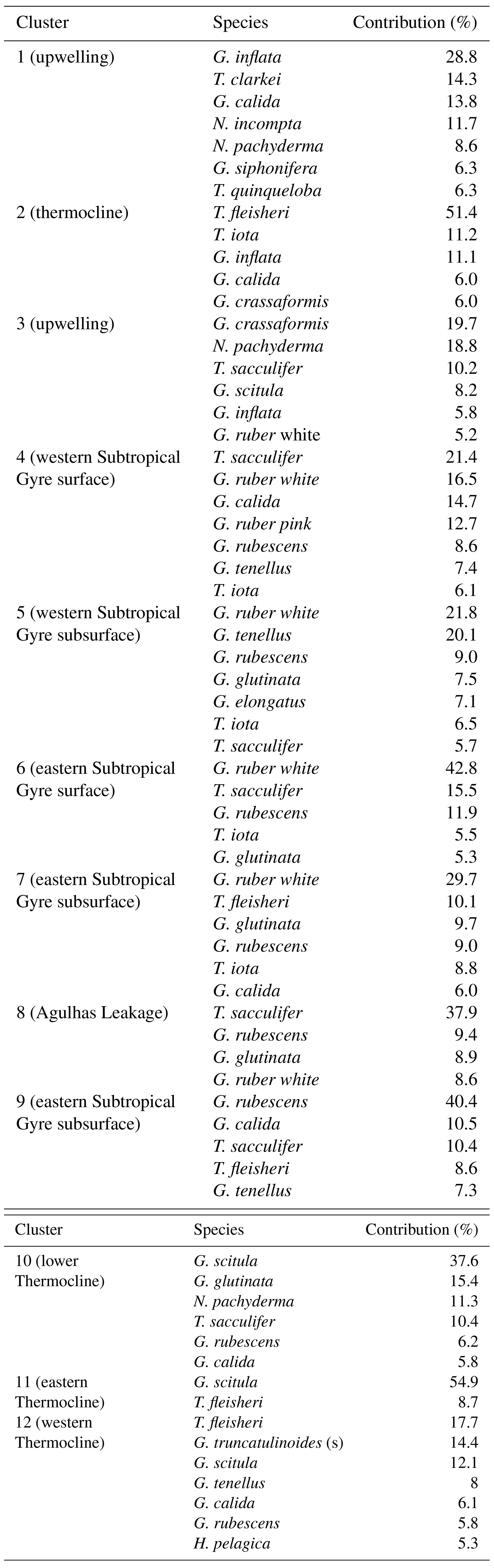
Table 3Contribution of most abundant planktonic foraminifera species (>5 %) in each cluster (given by average relative abundance).
4.2 Subtropical South Atlantic planktonic foraminifera communities
The distribution of species ALDs across the stations indicates the presence of three groups of species occupying different portions of the water column (Fig. 6). The upper 100 m layer is inhabited by upper and lower surface-dwelling species, separated from each other more distinctly in the center of Subtropical Gyre than in the Benguela region. This pattern was confirmed by the cluster analysis of the community composition for each depth and station, confirming the presence of five principal faunas, consistently separated by region and depth (Fig. 7). These were the Subtropical Gyre fauna that was further divided into surface (clusters 4 and 6), western subsurface (cluster 5), and eastern subsurface (clusters 7 and 9); the Agulhas Leakage fauna (cluster 8); the permanent thermocline fauna (clusters 2, 10, 11, and 12) that was further divided into western (clusters 2 and 12) and eastern (clusters 10 and 11); and finally the Benguela fauna (clusters 1 and 3). The average relative abundances for the most important species in each cluster are summarized in Table 3. This reveals that the warm and oligotrophic areas are inhabited by the same species, but that their proportions vary. The subdivision of the Subtropical Gyre fauna reflects increased abundance of G. rubescens and G. tenellus in the west and G. glutinata in the east. The Agulhas Leakage fauna was characterized by a high contribution of T. sacculifer and the presence of G. rubescens and G. tenellus. The Agulhas Leakage fauna was only present in the UML. At the LML, species belonging to the Benguela faunal cluster dominated the assemblages. Permanent thermocline and Benguela communities comprised distinctly different species groups. Permanent thermocline fauna is characterized by G. scitula, T. fleisheri, and G. truncatulinoides, whereas Benguela upwelling fauna is defined by G. crassaformis and N. pachyderma. The Benguela fauna also contained small contributions of G. inflata, N. incompta, and G. bulloides that are, in addition to upwelling conditions, also associated with the Subtropical Front. The deepest intervals at stations 394, 370, and 227 had too few or no living planktonic foraminifera and, therefore, could not be clustered.
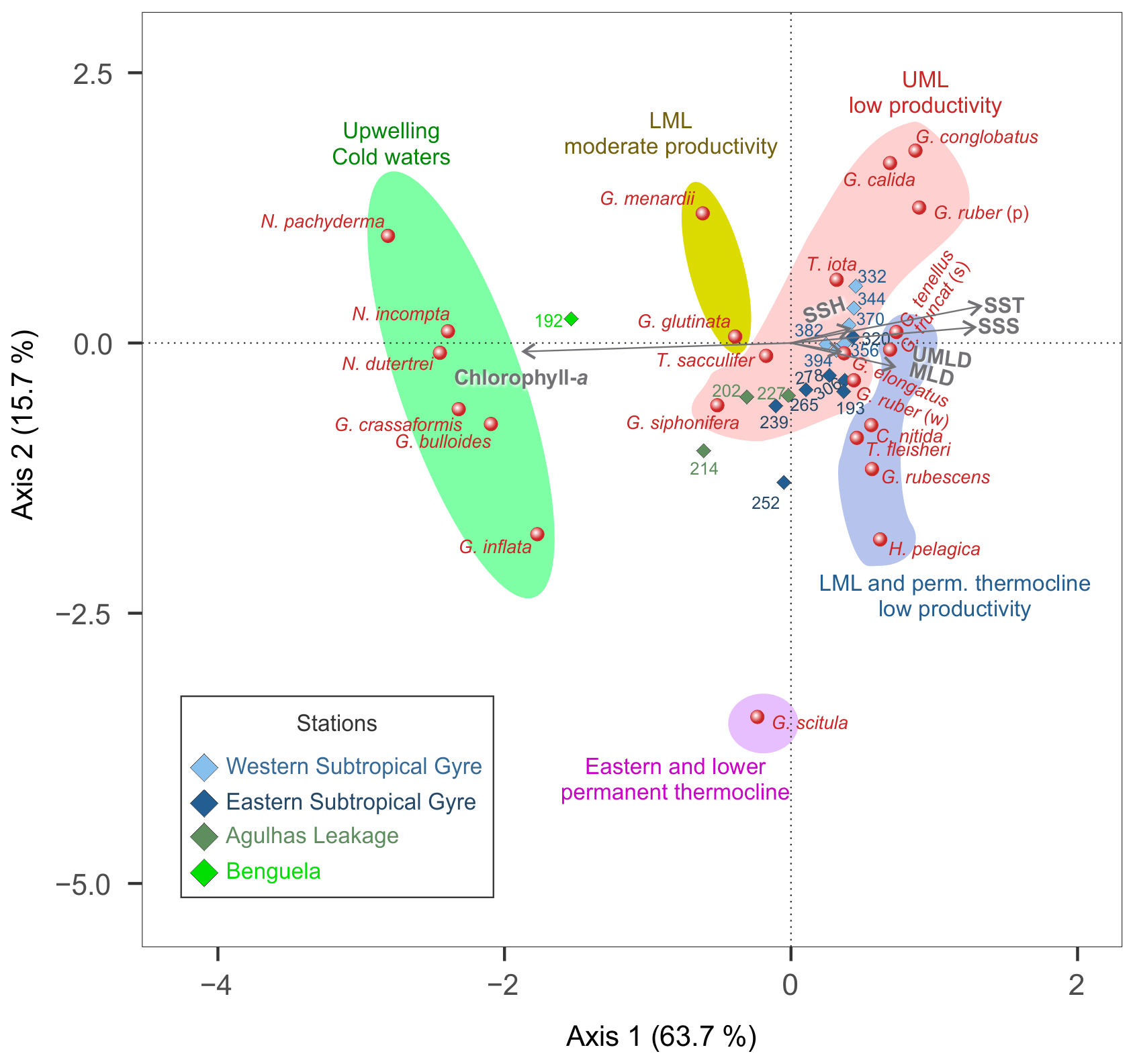
Figure 8CCA tri-plot of depth-integrated planktonic foraminifera assemblages from the M124 stations showing the position of species with at least 2 % in abundance and environmental parameters (UMLD – upper mixed layer depth; MLD – mixed layer depth, comprising UML and LML; SSH – sea surface height anomaly; SST – sea surface temperature; SSS – sea surface salinity).
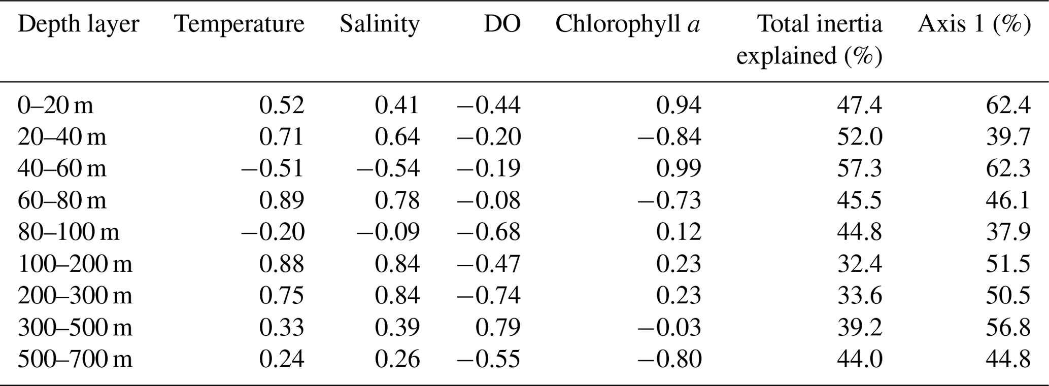
Table 4Depth-resolved CCA results, including the loadings of the four tested environmental parameters on the first canonical axis, the total proportion of inertia in the faunal composition explained by the constrained ordination, and the proportion of constrained inertia explained by the first CCA axis.
4.3 Variables and processes controlling the planktonic foraminifera distribution
The depth-integrated CCA shows that 68 % of the variability in species composition along the transect can be constrained by the tested environmental factors, with more than half of the total inertia being explained with two CCA axes (Fig. 8). The first axis (43 % of the total inertia) orients most species along a productivity–temperature gradient, with Benguela upwelling species on the high-productivity end and the warm surface and gyre subsurface species on the warm oligotrophic end. The second axis (11 % of the total inertia) appears to be related to the depth of the mixed layer and is responsible for the remaining variation in the non-upwelling faunas. It orients G. scitula at the extreme positive end opposite to G. ruber pink, G. calida, and G. conglobatus. Due to the distinct foraminiferal community in the Benguela upwelling system, station 192 stands out in relation to the other stations and hence may be responsible for a large proportion of the variability. Therefore, we carried out an additional analysis without this station, revealing that the negative correlation between SST and productivity remains at the ordination along the tested environmental variables and still explains more than half of the variability in species composition (Fig. S4), reflecting the fact that the Agulhas Leakage domain is also influenced by cold and productive waters below 40 m. Thus, the productivity vs. temperature gradient describes the faunal variation in the subtropical South Atlantic even outside of the Benguela upwelling.
Considering the importance of vertical gradients in environmental variables for the distribution of planktonic foraminifera in the subtropical South Atlantic, separate CCA(s) were performed on faunas from the nine depth layers (Fig. 9, Table 4 and Fig. S5 in the Supplement). These analyses revealed a pattern of vertical stacking in the relative contribution of the tested environmental factors on the planktonic foraminifera community composition. In the surface layer (0–60 m), chlorophyll a shows the highest absolute loading on the first CCA axis, and the four tested environmental variables together explain up to 57 % of the inertia in the fauna. Below 60 m, the tested variables explain less than 45 % of the total inertia, chlorophyll a concentrations cease to be the most important variable, and temperature becomes more important. The temperature–chlorophyll gradient, identified as the dominant control of the total faunal composition across the stations (Fig. 8), is manifested in the depth-resolved CCAs only between 20 and 80 m. It is not present at the surface (where chlorophyll a dominates) and below 100 m. Instead, from 80 m, dissolved oxygen concentration starts explaining a considerable amount of variance in the fauna, and between 80–100 and 300–500 m it appears most important. Temperature and salinity are the most important variables between 100 and 300 m, where the species are ordered along a temperature–oxygen gradient. Counterintuitively, the faunal variation at the deepest level (500–700 m) appears to be best explained by chlorophyll a concentration, but we note that the analysis at this depth level is strongly affected by the small number of living specimens and the resulting pattern should be interpreted with caution.
5.1 Synchronized reproduction and ontogenetic vertical migration
Before interpreting the vertical distribution of planktonic foraminifera in the water column as a function of changing environmental properties across the studied transect, it is important to evaluate the possible effect of reproductive processes on species concentration and living depth. The M124 cruise lasted for 16 d, with new moon occurring 10 d into the cruise, and the preceding full moon occurring 7 d before the sampling at the first station. If some of the species reproduced consistently in phase with full moon (Spindler et al., 1979; Jonkers et al., 2015; Venancio et al, 2016), then the proportion of preadult specimens should have been higher during the first half of the cruise. Three species show elevated abundance of preadults consistent with such a pattern: G. ruber white, O. universa, and G. calida (Bijma et al, 1990; Fig. S3). The remaining species show an even proportion of preadults throughout the cruise, which is not consistent with synchronized reproduction. However, when analyzed statistically, G. ruber white, O. universa and G. calida showed no systematic relationship between the proportion of preadults and lunar day, nor a periodic change in their ALD in phase with the lunar cycle, which speaks against a strict synchronization of their reproduction and provides no evidence for ontogenetic vertical migration. Hence, in the absence of a strong evidence for the control of reproductive or ontogenetic processes on the vertical habitat, and ruling out an effect of daily vertical migration based on detailed observations elsewhere (Meilland et al., 2019), we proceed by analyzing if the ALD of the individual species varied predictably as a function of environmental parameters.
5.2 Species vertical distribution across the subtropical South Atlantic
The ALD of planktonic foraminifera species shows a consistent depth ranking pattern and a mixture of stable and variable depth habitats (Fig. 5). Since the main feature of the water column relevant for the vertical distribution of non-motile plankton is the mixed-layer depth, we consider the observed ALD against this depth level (Fig. 6). First, we observe a group of species whose ALD was consistently in the Upper Mixed Layer (UML). Species in this group had an ALD shallower than 40 m and a low VD (up to 30 m) that usually did not range deeper than 40 m. This depth range corresponds to the extent of the warm thermal UML (Fig 2c). The most abundant species in this group were G. ruber (pink and white), G. conglobatus, O. universa, and T. sacculifer. These species all bear algal endosymbionts (Takagi et al., 2019), which likely explains their high abundances in the high-light and low-nutrient conditions of the UML. Such a shallow depth habitat of G. ruber was also observed by Berger (1968) and Rebotim et al (2017), but the ALDs for O. universa and G. conglobatus and also partly for T. sacculifer were shallower in the South Atlantic than in the North Atlantic (Schiebel et al, 2002; Rebotim et al., 2017; Jentzen et al, 2018), indicating that this species has a more variable habitat than observed in the studied section. Overall, our results confirm observations elsewhere that the dominant habitats of these species do not reach below the seasonal thermocline, indicating that they are constrained to the photic zone within the UML (Kemle-von-Mücke and Oberhänsli, 1999; Kuroyanagi and Kawahata, 2004; Rebotim et al, 2017; Jentzen et al, 2018).
A second group of species also preferentially inhabits the upper water layer (ALD usually shallower than 50 m), but their larger VD (up to 50 m) indicates that their habitat comprises the Whole Mixed Layer (WML). The most abundant species in this group are C. nitida, G. glutinata, G. calida, T. iota, G. rubescens, G. tenellus, and G. menardii. With the exception of T. iota, these species all bear algal endosymbionts (Takagi et al., 2019), which is consistent with their habitat within the photic zone. However, in contrast to the UML species group, these species appear less tightly linked to the surface layer, implying either a broader thermal tolerance or adaptation of their symbionts to lower light levels. Whereas for most species the observed habitat is comparable with previous work (Kemle-von-Mücke and Oberhänsli, 1999; Rebotim et al., 2017), the shallow habitat of T. iota is at odds with its concentration maximum around 300 m in the northeastern Atlantic reported by Rebotim et al. (2017), indicating a highly variable depth habitat that requires further investigation.

Figure 9Variable loadings for CCA carried out separately for the nine depth levels and the proportion of inertia constrained by the four tested environmental parameters. The shading shows the first axis loadings for each analyzed environmental parameter. The CCA outputs including the first CCA axis eigenvalue are shown in Table 4. Graphical outputs of each depth-separated CCA are shown in the Fig. S5 in the Supplement.
In contrast, species of the Lower Mixed Layer (LML) have a habitat that is still dominantly within the seasonal thermocline but whose vertical distribution overlaps with the deep chlorophyll maximum (Fig. 2c). The species in this group exhibit an ALD between 50 and 100 m and a VD similar to the UML group. The most abundant species in this group were G. elongatus, N. dutertrei, N. pachyderma, N. incompta, G. crassaformis, and G. inflata. With the exception of G. elongatus, these species occurred in the Agulhas Leakage and Benguela stations, indicating that this group may respond primarily to variations in productivity, since there the chlorophyll a concentration was higher, the DCM shallower, and the water column less stratified (Fig. 2c). At station 192, which is influenced by Benguela upwelling, the planktonic foraminifera community was dominated by the LML group at all vertical levels. The species G. elongatus was the only LML species in the Subtropical Gyre. This species was the most abundant of the Globigerinoides plexus, but we caution against a too strict interpretation of its apparently substantially deeper habitat than the other from the Globigerinoides plexus because the species could only be distinguished in its adult stage (Aurahs et al., 2011; Morard et al, 2019), and its apparently deeper habitat may reflect the habitat of adult specimens only. Nevertheless, the observed depth stratification between G. elongatus and G. ruber (white) is consistent in sign with previous studies based on observations in the plankton (Kuroyanagi and Kawahata, 2004) and oxygen isotope and Mg∕Ca ratios (Wang, 2000; Steinke et al., 2005). Thus, at least in summer, adult G. elongatus live below the UML in the South Atlantic.
Species of the “Thermocline” group show a distinctly different ALD distribution, with the largest part of the population occurring below the seasonal thermocline. Species in this group have a variable ALD within the permanent thermocline (deeper than 100 m) that is in general independent of the position of the DCM. In fact, most of their populations occur often below the DCM. The most abundant species belonging to this group are T. fleisheri, G. truncatulinoides, G. scitula, and H. pelagica. Thermocline-dwelling species represent a clearly defined group distinct from other species assemblages (Fig. 6), suggesting that they constitute a distinct community that may not be shaped by surface processes. Since photosynthesis is inhibited due to insufficient light within their habitat, species of the thermocline group are likely to feed on either zooplankton or sinking organic matter (Schiebel and Hemleben, 2017). Little is known about the ecological preferences of T. fleisheri because this species is small and hence often overlooked as most studies only investigate the specimens >150 µm. Rebotim et al (2017) classified T. fleisheri as a surface to subsurface dweller. However, the species was rare in their study, rendering this classification uncertain. In our transect, T. fleisheri was abundant between 100 and 300 m at all Subtropical Gyre stations with specimens up to 200µm in size (see Plate A5, 11–13). Within the Subtropical Gyre, the ALD of T. fleisheri was close to the DCM in 10 out of 13 stations within the subtropical Gyre, suggesting a link between depth habitat and the depth of the chlorophyll maximum for this species (Fig. 5). The ALD of G. scitula was the deepest (235 m) and most variable (VD 109 m) in our study. The mesopelagic habitat of G. scitula has also been observed elsewhere (Bé and Tolderlund, 1971; Itou et al, 2001; Field, 2004; Storz et al, 2009; Rebotim et al, 2017; Jentzen et al, 2018). This demonstrates that the species is a consistent permanent thermocline dweller, living below the deep chlorophyll maximum. The species G. truncatulinoides had an ALD near 170 m with a relatively low VD (55 m), which associates it to the lower part of the DCM and the permanent thermocline below. The cytoplasm color of G. truncatulinoides was similar to G. scitula (see Plates A4 and A5) perhaps indicating a similar diet. However, the spatial distribution of the two species shows that G. truncatulinoides replaces G. scitula towards the west at stations in the Subtropical Gyre; similar to the Azores Current System where G. truncatulinoides linked to North Atlantic Subtropical Gyre is replaced by G. scitula when transitional waters from the Azores Front migrated southwards (Storz et al, 2009). The habitat of H. pelagica is dominantly subsurface but highly variable, perhaps reflecting the presence of both the surface and the subsurface genetic types of this species (c.f. Weiner et al., 2012).
5.3 Depth hierarchy of relationships between planktonic foraminifera and environmental parameters
Plankton net samples represent a snapshot of the plankton state in space and time. In this way they allow us to observe the direct response of the plankton community to environmental parameters. This is fundamentally different from relationships extracted from sedimentary assemblages, which represent long-term (years to millennia) integrated fluxes of species (Jonkers et al., 2019). Temperature appears to be the dominant parameter explaining variation in community composition in sediment assemblages (Morey et al., 2005). However, sedimentary assemblages result from vertical and temporal (seasonal) integration of assemblages, and the effect of temperature on their composition may therefore be indirect. Indeed, our results confirm earlier suggestions (Schiebel and Hemleben, 2000; Schiebel et al, 2001) that abiotic and biotic parameters other than temperature play an important role in explaining the distribution of planktonic foraminifera in the water column. Both the habitat depth variability among species (Figs. 5, 6) and the distribution of the species along the transect (Fig. 7) provide clear hints for the effect of multiple environmental parameters on the habitat and the abundance of the species. These hints are reinforced by the results of the CCA (Fig. 8), where the first axis sorts the community according to the productivity in the mixed layer. The subtropical gyre stations are further separated along the second dimension of the CCA, which appears to be related to the vertical gradient in the water column. This separation is mirrored by a distinct grouping of species characterizing the end-members of the CCA gradient (Fig. 8). SSH does not appear to systematically affect the species distribution, indicating that the observed spatial pattern is not affected by the presence of eddies or Agulhas Rings with distinct fauna (Peeters et al., 2004) carried far into the South Atlantic.
The analysis of species distribution along the transect (without the two easternmost stations) separately for each of the nine depth layers provides further details on how the vertical structure of the water column affects the assemblages. This analysis reveals the presence of a vertical hierarchy of environmental parameters affecting community composition (Fig. 9), indicating that the vertical changes in the community composition shown by the cluster analysis (Fig. 7) may be the consequence of the vertically varying importance of environmental factors. The UML fauna has an affinity for high light and high temperatures, but variations in the composition of the communities in the uppermost layer along the studied transect seems to be driven by chlorophyll a concentration. This may hint at differences in the adaptation of the UML fauna with respect to productivity. From the LML, the influence of physical oceanographic parameters on the composition of the WML and LML faunas become visible, with temperature and salinity displaying higher loadings on the first CCA axis. The importance of chlorophyll a concentrations is reduced below 60–80 m and the variation in the LML and Thermocline faunas is less well explained by the CCA models (inertia explained dropping to below 40 %) and requires combinations of multiple variables, including DO, with temperature and salinity linked to DO and chlorophyll a with different signs at different depth levels.
Considering the actual DO values, the role of this parameter must be indirect, as O2 concentrations throughout the studied water column are far above levels at which foraminifera species begin to display differential adaptations ( for benthic foraminifera, Kaiho, 1999; see also Kuroyanagi et al., 2013) and therefore cannot have a direct physiological effect. The relationship therefore likely arises from collinearity with other environmental and/or biotic factors. Indeed, the apparent importance of chlorophyll a at depths where it no longer can reflect primary production and the effect of DO at concentrations which cannot incur a direct physiological effect both point to processes related to food availability. Such processes (e.g., aggregate composition and abundance) are not captured directly by any of the tested variables and the presence of additional, untested controls on the assemblage is indicated by the lower portion of the faunal variance explained by the ordinations at those depths (Fig. 9). We therefore infer that abundance and quality of food, and perhaps the interaction with other plankton, likely play an important role in shaping planktonic foraminifera community within the permanent thermocline. Dietary preferences of thermocline-dwelling species are poorly known, although indirect observations of N. dutertrei indicate an affinity with marine snow (Schiebel and Hemleben, 2017; Fehrenbacher et al, 2018).
Whatever the exact environmental and biotic controls on community composition at depth may be, the existence of a vertical succession of parameters constraining community composition of planktonic foraminifera adds a new dimension to ecological models derived from sedimentary assemblages (transfer functions) and the inverse efforts to model planktonic foraminifera assemblages from upper ocean properties. Our results reinforce the notion that even though near-sea-surface temperature appears the best predictor of sedimentary assemblages, this relationship may not be always direct and may at least in part arise from the integration of vertically (and seasonally) separated assemblages. Theoretically, it should thus be possible to extract information on vertical characteristics of the past water column through targeting specific species groups. For example, the progressive replacement of G. scitula by G. truncatulinoides observed between eastern and western thermocline faunas is clearly not driven by temperature (Figs. 2 and 7), and if this replacement is preserved across the seasonal cycle, it could be an indication for the properties of subsurface waters in the South Atlantic.
We investigated the zonal and vertical distribution of planktonic foraminifera at 17 stations across the subtropical South Atlantic during the late austral summer 2014. Using in situ vertically resolved environmental data we assessed which factors drive the observed foraminifer species distribution.
-
Species-specific standing stocks varied regionally, with the most pronounced differences among communities observed between Benguela (station 192) and Subtropical Gyre (stations from 394 to 239), with an intermediate community in the Agulhas Leakage region (stations from 227 to 202).
-
The highest standing stock was observed in the upper 60 m of the water column, whereas the numbers of dead specimens (no cytoplasm) increased below 100 m. The highest concentrations of planktonic foraminifera occurred at stations in the oligotrophic western Subtropical Gyre, indicating that the total standing stock is not positively correlated with productivity during the summer.
-
We observed no strong evidence for synchronized reproduction affecting the species distribution, and a distinct pattern of species-specific habitat depth, resulting in the existence of distinct vertically stratified faunas.
-
The permanent thermocline layer hosts a planktonic foraminifera community distinct from the mixed layer. In the western South Atlantic, high abundances of G. truncatulinoides, T. fleisheri, and G. scitula were observed, whereas G. scitula dominated the community in the eastern South Atlantic. Zonal differences in the mixed layer communities were less pronounced.
-
Overall, the zonal distribution of species was primarily affected by the inverse relationship between chlorophyll a and water temperature, and secondarily by the vertical structure of the water column in the Subtropical Gyre.
-
The vertical distribution of planktonic foraminifera showed a clear depth-dependent hierarchy in the environmental parameters explaining assemblage variability. The variability in the upper 60 m was mainly influenced by productivity (chlorophyll a). Below 60 m, the community composition was more difficult to explain by the tested variables and we infer that next to temperature (and salinity) the abundance and quality of food (or other biotic interactions) likely played an important role.
Overall, planktonic foraminifera communities of the subtropical South Atlantic seem to respond to a horizontally and vertically variable combination of environmental parameters. This should be taken into account when interpreting sedimentary assemblages and in efforts to model foraminifera production from environmental parameters.
Description and plates of main planktonic foraminifera species found during the M124 cruise. Plates are provided as Plates A1–A5.
Spinose species
Globigerinella calida Parker (1962) (Plate A1, 1–2)
Specimens with very low trochospiral coiling. The last whorl comprises four to five chambers that rapidly increase in size. Chambers are elongated and clearly separated with a spined and cancellated surface. Sutures are slightly curved and deep in both umbilical and spiral sides. The main aperture is extraumbilical with a long arch (0.25 circle) from the umbilicus to the periphery bordered by a lip. Preadult specimens have the same morphological characteristics as adult specimens. Living specimens have a brownish stained cytoplasm.
Globigerinoides conglobatus Brady (1879) (Plate A1, pictures 3–5)
Only immature adult specimens of G. conglobatus were found during the cruise. Specimens were marked by low trochospiral coiling with four rough and densely spined chambers in the last whorl. All chambers were spheric in preadult specimens (Plate A1: picture 5), immature adult specimens have a slight flattened last chamber (Plate A1: pictures 3 and 4). The main aperture is umbilical, a low arch bordered by a rim similar to Globigerina bulloides in adult specimens. The primary aperture of preadult specimens is droplet shaped arch slightly displaced from the umbilicus. There are two small supplementary apertures by chamber in the spiral side, which are placed near to each other and they are visible in both adult and preadult specimens. Living specimens have a brownish stained cytoplasm. Preadult G. conglobatus is distinguished from G. calida by the umbilical aperture and the presence of supplementary apertures in the spiral side. G. conglobatus can be differentiated from G. bulloides by the rough and densely spined chamber's surface, and/or by the presence of supplementary apertures in the spiral side.
Globigerinoides ruber d'Orbigny (1839) (Plate A1, pictures 6 -13)
Adult specimens of G. ruber had low or moderate trochospiral tests, with large size and three spherical and symmetric placed chambers in the last whorl. Most of specimens presented a ruber-type wall structure (rougher than G. bulloides, but less than G. calida or Globoturborotalita rubescens, Schiebel and Helembem, 2017) with spines. Most of the specimens found in the Agulhas Leakage and Benguela realms presented sacculifer-type wall structure (honeycomb-like spines base, Schiebel and Helembem, 2017) wall surface. The primary aperture is an umbilical semicircular arch centralized over the suture of the two previous chambers. Two secondary apertures are found in the spiral side placed moderately far to each other. Preadults specimens diverge to adult specimens, their tests presented 3.5 (neanic stage)–4.5 (juvenile stage) chambers in the last whorl. The surface is composed of very few spines and pores and looks microperforate in the stereomicroscope view. The primary aperture is umbilical–extraumbilical, reaching the periphery in juvenile specimens and migrating to the center in posterior ontogenetic states. No secondary apertures are visible in the spiral side. Living G. ruber specimens presents a brownish cytoplasm. Adult G. ruber pink specimens present bright pink chambers, and preadult specimens present pallid to bright pink chambers. It is difficult to separate preadult G. ruber pink and preadult G. rubescens, the best way is to observe the equatorial periphery that tends to follow both adult G. ruber and G. rubescens. These same properties can be used to separate the neanic stage of G. ruber from the late neanic stage of Trilobatus sacculifer. The neanic stage of G. ruber white can be separated from Globigerinita glutinata in stereomicroscope view by the presence of a semicircular primary aperture in G. ruber and the brownish cytoplasm.
Globigerinoides elongatus (Plate A1, pictures 14 and 15)
The test morphology is the same than for G. ruber. G. elongatus is distinguished from G. ruber white by the flattening of chambers, especially the last one. The primary aperture is a reverse U-shaped arch in spite of a perfect semicircular G. ruber aperture. G. elongatus also presents a less deep umbilicus than G. ruber white. Living specimens presented a brownish cytoplasm. Preadult G. ruber and G. elongatus cannot be easily distinguished.
Trilobatus sacculifer (Plate A2, pictures 1–6)
Test with a large size and low trochospiral coiling with a sacculifer-type wall structure in adult specimens. Immature adult specimens (variants T. trilobus, T. immaturus, and T. quadrilobatus) have spheric lobular chambers, 3.5 in the last whorl. Mature adult specimens (variant T. sacculifer) present an elongated sac-like last chamber and four chambers in the last whorl. Chambers are rather separated and increase in size quickly. In immature adult specimens, the umbilicus is narrow and the primary aperture is interiomarginal umbilical, a long arch bordered by a rim. In mature adult specimens, the primary aperture is a more pronounced arch centralized over the third chamber, bordered by a rim. Adult specimens present one supplementary aperture by chamber in the spiral side. The morphology of preadult T. sacculifer diverges from adults. Early neanic specimens present a nearly smooth wall structure with six or more compacted globoid chambers. Late neanic specimens present four chambers in the last whorl, the sacculifer-type wall structure is already present, but the equatorial view resembles more Globorotalia inflata than a typical Globigerinoides. The primary aperture is equatorial in juvenile specimens (Schiebel and Hemleben, 2017), migrating to umbilicus in the next ontogenetic states. In neanic specimens, the primary aperture is interiomarginal; a nearly semicircle arch bordered by a rim and no supplementary aperture is visible. Late neanic T. sacculifer differs from neanic G. ruber white due to the Globorotalia inflata-like chambers and having more chambers visible in the spiral side.
Globoturborotalita rubescens Hofker (1956) (Plate A2, pictures 7–9)
Specimens are small or medium sized, with low to medium trochospiral test and ruber-type wall structure. The axial view is diamond-shaped with four chambers in the last whorl. Chambers are globoid and spheric with a cancellate surface and small size increase by chamber. The primary aperture is umbilical, with a semicircle arch bordered by a rim. No supplementary aperture visible. Preadult individuals present five to six nearly smooth chambers in the last whorl and an umbilical–extraumbilical aperture. Specimens have pink-stained chambers in general, the living ones present brownish cytoplasm and more pronounced pink-stained chambers. It is difficult to differentiate G. rubescens and neanic G. ruber pink and white. The difference is the diamond-shaped axial periphery. Preadult G. rubescens present more visible chambers in the juvenile whorl than G. ruber.
Globigerinoides tenellus Parker (1958) (Plate A2, pictures 10 and 11)
Tests are morphologically similar to G. rubescens. Specimens of G. tenellus have more cancellate chambers and are never pink stained. The primary aperture's arch is a reversed U-shape and there exists a supplementary aperture in the spiral side, which is not always easily visible.
Orbulina universa d'Orbigny (1839) (Plate A2, pictures 12 and 13)
Mature adult specimens of O. universa have a large size with a single spheric chamber that covers the whole organism. The chamber is translucent and presents pores of diverse sizes and some spines. Pores and the observation of previous Globigerina-like growing inside the spheric chamber are some features that allow for distinguishing O. universa from spherical Radiolarians. Immature adult specimens present a Globigerina-like shape with a low trochospiral test, four chambers in the last whorl and an umbilical aperture, and a long arch sometimes bordered by a rim that covers almost all previous chambers (similar to Globigerina bulloides). In some tests, a supplementary aperture in the spiral side was observed. Chambers are smooth and very delicate and fragile, which can be broken with a moderate brush pressure. Living O. universa has a brownish cytoplasm and very dark brownish cytoplasm in immature adults. Preadult O. universa specimens were also present in the M124 collection; they differ from immature adults by having five chambers in the last whorl and a nearly planispiral test, which differs from G. calida and G. siphonifera due to its smooth and very fragile chambers.
No spinose and macroperforate species
Genera Neogloboquadrina (Plate A3, pictures 1–7)
Individuals of N. dutertrei and others Neogloboquadrinid species of the M124 collection were found in the easternmost stations belonging to Benguela and Agulhas Leakage fauna. Neogloboquadrinid species tended to diverge morphologically from global Neogloboquadrina pattern.
Neogloboquadrina dutertrei d'Orbigny (1839) (Plate A3, pictures 1–3)
Individuals are medium to large sized with a low trochospiral. Rounded axial view. Chambers with a ridge-like wall structure (Neogloboquadrina type) and 4.5 or more unities in the last whorl. The morphology of chambers in M124 specimens diverged from the expected Neogloboquadrina pattern. They are more spheric and separated. Umbilicus opened and the aperture of two or three last chambers covers the upper side. The aperture is interiomarginal extraumbilical, sometimes with a tooth-like structure. Living individuals presented a hazel-greenish cytoplasm. Tests with 4 or 4.5 chambers in the last whorl were considered N. dutertrei only if the tooth-like structure was present inside the aperture.
Neogloboquadrina incompta and Neogloboquadrina pachyderma (Plate A3, pictures 4–7)
N. incompta and N. pachyderma were classified according to specimen coiling direction. Right-coiling specimens were classified as N. incompta, and left-coiled specimens were classified as N. pachyderma. Tests with the size varying from small to medium with low trochospiral. The axial periphery is squared, with 4 or 4.5 chambers in the last whorl. N. incompta and N. pachyderma specimens of the M124 cruise collection present the Neogloboquadrina-type wall structure. However, this feature demanded more than 100× magnification in order to be visualized under the stereomicroscope. At magnification, the tests look smooth, similar to microperforate species. Similar to N. dutertrei, chambers of N. incompta and N. pachyderma were much more spheric and separated from each other, diverging from the typical Neogloboquadrina pattern. Umbilicus is almost closed and the primary aperture is interiomarginal extraumbilical, with an almost straight arch with a pronounced lip. Living individuals presented a transparent or pallid green cytoplasm color. Tests of N. incompta or N. pachyderma were distinguished from N. dutertrei with 4 or 4.5 chambers in the last whorl if the aperture was bordered by a lip and the test presented a squared axial periphery and a very smooth surface. The extraumbilical aperture with a lip and the moderate chamber size increase allowed us to differentiate these atypical smooth tests from Globigerinita glutinata and Tenuitella iota in low stereomicroscope magnification.
Globorotalia crassaformis (Plate A3, pictures 8–10; plate A4, pictures 1–3)
Individuals of G. crassaformis were encountered rarely in the Subtropical Gyre (western side of the transect) stations and in low abundances in Agulhas Leakage and Benguela (eastern side of transect) stations. However, test morphology differed strongly between western (Subtropical Gyre) and eastern (Agulhas Leakage and Benguela) stations. Specimens classified as G. crassaformis have a very low trochospiral test with a flat spiral side and a conic umbilical side. The outline is angular with a squared appearance. The equatorial border is sharp, giving a plane convex aspect if viewed from the side. Specimens present 4–4.5 chambers in the final whorl. Chambers are smooth with visible pores in the spiral side and pustules in the umbilical side forming a strong calcite crust. Sutures are strongly curved in the spiral side and almost straight in the umbilical side.
In specimens from the Subtropical Gyre (Plate A4, pictures 1–3), the chamber border is strongly sharpened with a keel appearance, with strictly four unities in the last whorl. The umbilical view resembles Globorotalia truncatulinoides, with the aperture inside the umbilicus, which is an interiomarginal extraumbilical slit with a lip. Living individuals presented a strong dark hazel-stained cytoplasm. Those specimens can be separated from G. truncatulinoides by having four chambers in the last whorl and a squared outline.
In specimens from Agulhas Leakage and Benguela faunas (Plate A3, pictures 8–10), the chambers have a slight globular shape, but they still maintain a concave side view. Most of them were small individuals with 4.5 chambers in the last whorl. The umbilical view resembles Globorotalia inflata, but the aperture is a short semicircle arch. Living specimens presented a pallid green-stained cytoplasm. Those individuals can be differed from G. inflata by having more than four chambers in the last whorl, a plane convex side view, curved sutures in the spiral side, and a short arch of the aperture.
Globorotalia menardii (Plate A4, pictures 4–6)
Tests are very low trochospiral, rounded outline with a peripheral keel, and a very bi-flat side view. Chambers are smooth with pores and flat and sharp with five or six unities in the last whorl. Some carbonate pustules are common near the aperture. Sutures curved and keeled in the spiral side, and are slightly curved and deepen in the umbilical side. The aperture is interiomarginal extraumbilical, with a slit arch bordered by a lip. Some specimens presented a flap extending on the aperture. Living specimens presented a greenish cytoplasm with a strong red spot in early chambers.
Globorotalia inflata (Plate A4, pictures 7–9).
Tests are very low trochospiral and in general medium sized. The outline is slightly angulated and the side view is a not sharp plane convex. Chambers are globoid, smooth with some tooth-like calcite pustules, bean-shaped in the spiral side, and triangle-shaped in the umbilical view, with three to four unities in the last whorl. Sutures are very slight curved and deepen in both the spiral and umbilical side. The aperture is a long arch that is interiomarginal extraumbilical and sometimes bordered by a rim. Living specimens contain a pallid green or light hazel cytoplasm. G. inflata was found only in Agulhas Leakage and Benguela stations occupying the subsurface and upper thermocline layers. Despite the uneasy identification, individuals of G. inflata can be differed from eastern G. crassaformis by presenting three chambers in the last whorl, globoid chambers, a smoother surface, very slight curved sutures, and a big aperture in long arch.
Globorotalia scitula (Plate A4, pictures 10–12)
Tests are very low trochospiral, rounded outline without keel, and a biconvex side view. Chambers are smooth with big pores, a sharp border, and five unities in the last whorl. Sutures are very curved and almost flat in the spiral side and slightly curved and deepened in the umbilical side. The aperture is an interiormarginal, extraumbilical slit bordered by a lip. Living individuals had a dark hazel cytoplasm. G. scitula differed from G. crassaformis by having more chambers in the last whorl, a nearly flat biconvex side view, and a rounded outline.
Globorotalia truncatulinoides (Plate A5, pictures 1–3)
Tests are very low trochospiral and conic, and adults reach more than 400 µm. The spiral side is flat and the umbilical side is triangular, giving a plane convex (cone-shaped) side view. The outline is very round with a thick keel. Chambers are pyramidal, keeled border calcite encrusted umbilical side by high number of pustules, five unities in the last whorl. The umbilicus is deep, similar to a volcano crater in some specimens. The aperture is located in the bottom of the umbilicus, an interiomarginal, extraumbilical slit bordered by a lip. Living specimens presented a brown to dark hazel cytoplasm. G. truncatulinoides differs from G. crassaformis of the Subtropical Gyre by having a round outline, five chambers in the last whorl, and a thick peripheral keel. Regarding the genetic types (Vargas et al, 2001), M124 specimens had many spike-shaped calcite crusts suggesting higher morphologic similarity with genetic type 2 than type 3, although most of specimens were left-coiled.
Microperforate non-spinose species
Globigerinita glutinata (Plate A5, pictures 4 and 5)
Test are low trochospiral and small or medium sized. The wall structure is smooth with very small calcite pustules, pores are not visible under the stereomicroscope, with 3.5 or 4 chambers in the last whorl. Chambers are globoid and spheric, compressed on each other, and moderately increased in size. Mature adults of G. glutinata develop a “bulla” last chamber over the umbilicus, but it was very rare in the M124 collection. Umbilicus is near to closed and the primary aperture is umbilical, with a very narrow arch bordered by a lip or rim. A secondary aperture in the spiral side may be present in the last chamber of some specimens. Living specimens had a green- or orange-stained cytoplasm. Preadult specimens differ morphologically from adults, but they cannot be differentiated easily from preadults of Tenuitella species and immature Turborotalita clarkei under the stereomicroscope.
Candeina nitida (Plate A5, pictures 6–8)
Tests are low trochospiral and medium to large in size. The wall structure is very smooth, with very few calcite pustules, giving a transparent and reflective surface. Micropores are not visible under the stereomicroscope. There are three chambers in the last whorl, which are globoid, spheric, and compressed. Adult specimens do not present a unique primary aperture. Instead, several sutural small apertures are present. Preadult specimens present a small primary aperture and resemble G. glutinata, which can be distinguished by the much smoother surface and the persistence of three chambers in the juvenile whorl (visible on the spiral side). Living adult specimens presented between green- and orange-colored cytoplasm.
Tenuitella iota (Plate A5, picture 9)
Tests are low trochospiral and tiny to small in size. The wall structure is smooth with many thick spike-shaped calcite pustules. Micropores are not visible under the stereomicroscope. Chambers are globoid spheric and separated from each other, with four unities in the last whorl. Mature adults of T. iota develop a “bulla” last chamber over the umbilicus, but no specimens with this feature were observed in the M124 collection. The primary aperture is umbilical–extraumbilical, with a short arch bordered by a rim. Living specimens contain a green- to hazel-colored cytoplasm, with orange- or red-stained early chambers. Adults of T. iota differ from G. glutinata by presenting thick and spike-shaped calcite pustules and more separated chambers. Preadult specimens have five chambers in the last whorl, globoid chambers with a flattened side view, and an extraumbilical aperture, but other preadult Tenuitella species and G. glutinata present a similar morphology, making the separation difficult.
Tenuitella fleisheri (Plate A5, pictures 10–12)
Tests are low trochospiral and tiny to medium in size (up to 200 µm). The wall structure is smooth, and some specimens present few calcite pustules, while others specimens have many. Chambers are flattened globoid, elongated, and become slightly ampullate in mature adults. The growing morphology shows four to five separated chambers in the last whorl with a moderately increasing rate. The aperture is interiomarginal extra umbilical with a flap-like lip. There is no difference between preadult and adult specimens, but other preadult Tenuitella species and G. glutinata present a similar morphology, hampering the separation. Living individuals presented greenish hazel or hazel-colored cytoplasm. Adult T. fleisheri differ from T. iota by having a flattened side view. Adult T. fleisheri differ from T. parkerae by not having pronounced elongated chambers and more calcite pustules on the surface.

Plate A1(1) Adult and (2) preadult stages of Globigerinella calida. (3, 4) Adult and (5) preadult specimens of Globigerinoides conglobatus. (6, 7) adult and (8) neanic specimens of Globigerinoider ruber pink. (9–13) Globigerinoides ruber white in different ontogenetic states: (9, 10) adult, (11, 12) neanic, and (13) juvenile. (14, 15) Adult Globigerinoides elongatus.
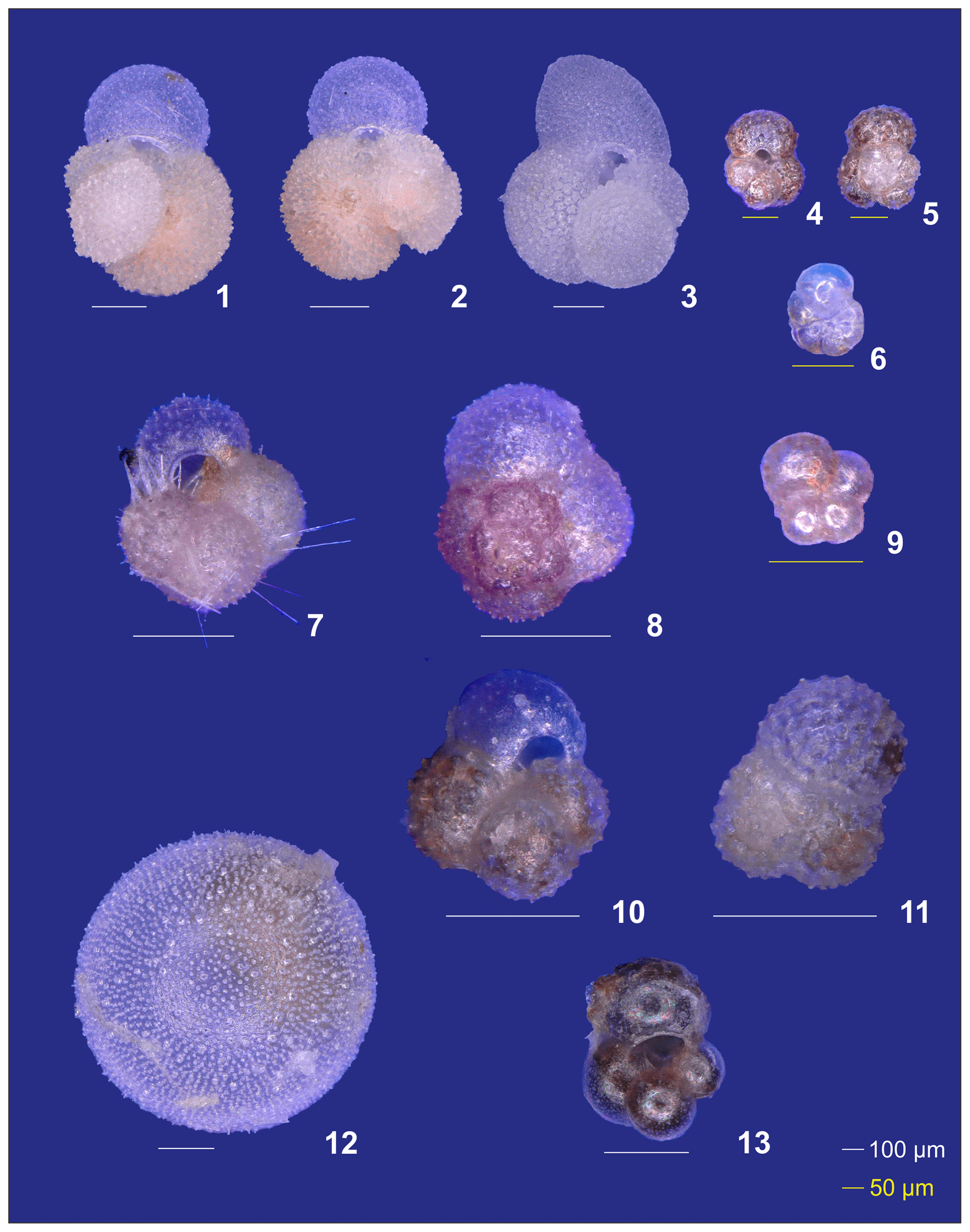
Plate A2(1–6) Different ontogenetic stages of Trilobatus sacculifer: (1, 2) adult without sac, (3) adult with sac, (4, 5) late neanic, and (6) early neanic. (7–9) Globoturborotalita rubescens: (7, 8) adult and (9) preadult. (10, 11) Specimens of Globigerinoides tenellus. (12) Late adult Orbulina universa with the final spheric chamber, and an (13) early adult Globigerina-like specimen with soft and smooth chambers.
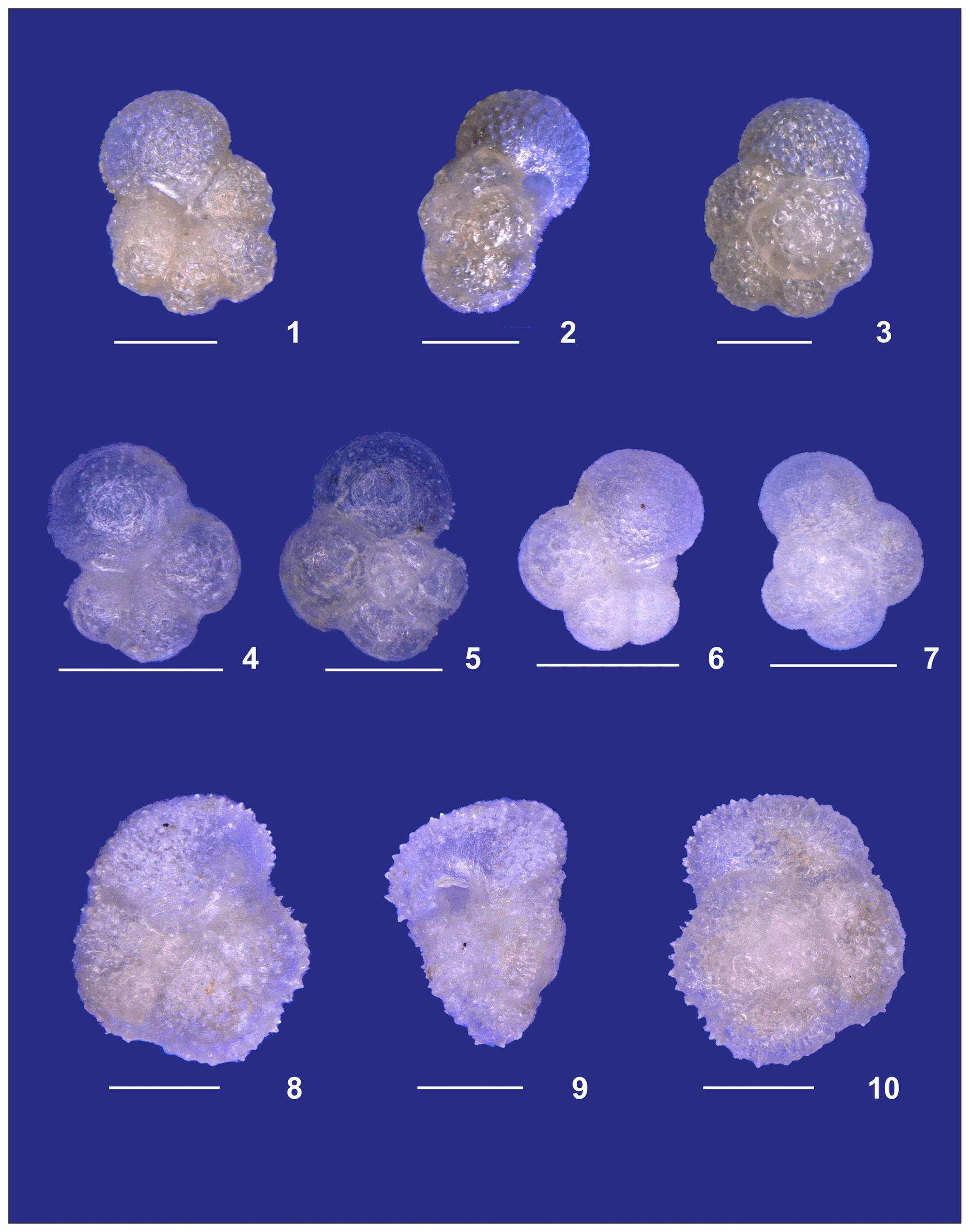
Plate A3(1–3) A small specimen of Neogloboquadrina dutertrei. (4, 5) Neogloboquadrina incompta and (6, 7) Neogloboquadrina pachyderma. (8–10) Adult Globorotalia crassaformis sensu lato from station 192 (Benguela). White bars for overviews are 100 µm.
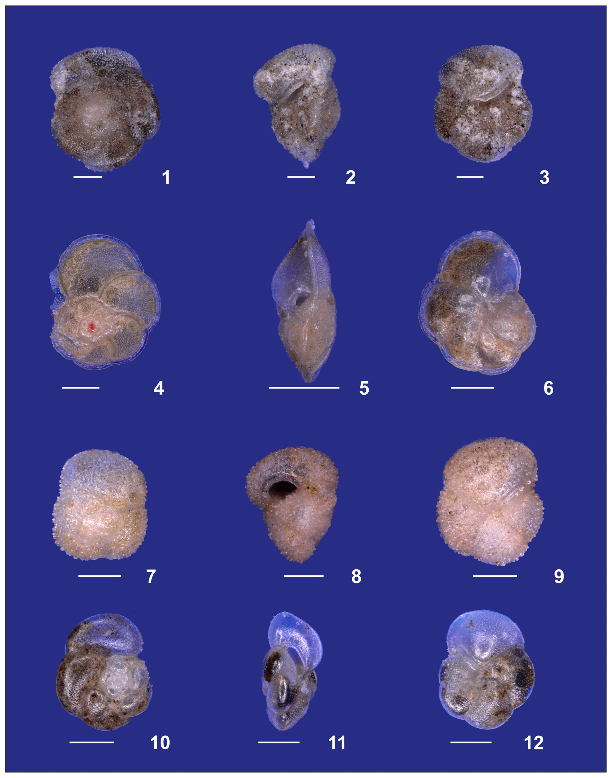
Plate A4(1–3) Adult Globorotalia crassaformis sensu stricto from station 382 (western Subtropical Gyre). (4–6) Adult Globorotalia menardii. (7–9) Globorotalia inflata. (10–12) Globorotalia scitula. White bars for overviews are 100 µm.
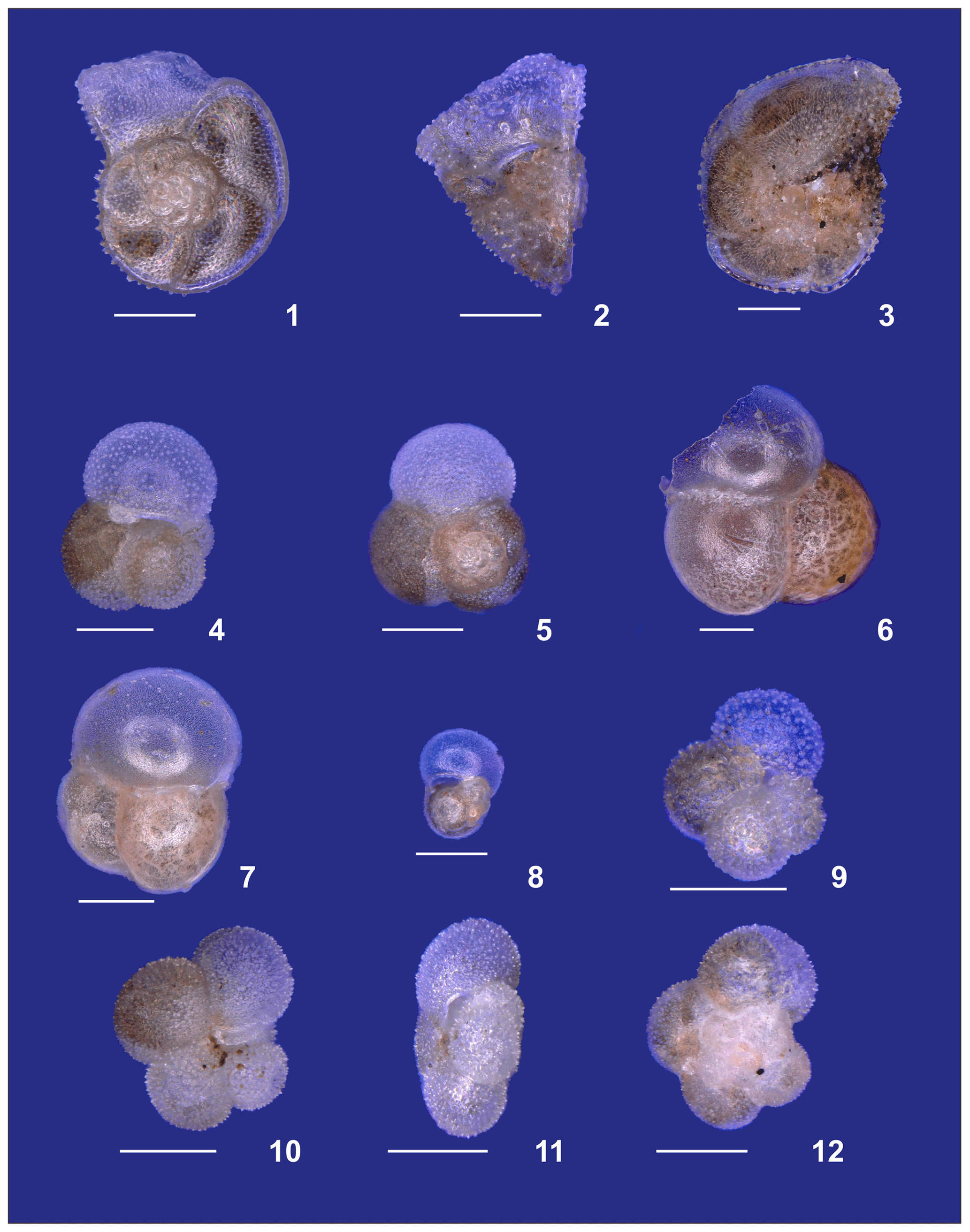
Plate A5(1–3) Adult Globorotalia truncatulinoides. (4, 5) Adult Globigerinita glutinata. (6, 7) Adult and (8) preadult specimens of Candeina nitida. (9) Tenuitella iota. (10–12) Tenuitella fleisheri. White bars for overviews are 100 µm.
The foraminifera concentration data have been deposited at PANGAEA (https://doi.pangaea.de/10.1594/PANGAEA.920553, Lessa et al., 2020). CTD data from the M124 cruise are available on PANGAEA: https://doi.org/10.1594/PANGAEA.895426 (Siccha et al., 2018) and https://doi.org/10.1594/PANGAEA.863015 (Karstensen and Krahmann, 2016). SSALTO/DUACS sea surface height data were obtained from https://www.aviso.altimetry.fr/en/data/ (CNES Aviso+, 2018).
The supplement related to this article is available online at: https://doi.org/10.5194/bg-17-4313-2020-supplement.
DL analyzed the planktonic foraminifera fauna and was responsible for the manuscript writing. RM was responsible for collection of planktonic foraminifera during the cruise and contributed to the oceanographic data analyses. LJ contributed to the statistical analyses. IGV contributed to the interpretation of the lunar periodicity on planktonic foraminifera species. RR and AB contributed to the collection of planktonic foraminifera during the cruise. ALA headed the Paleoceano project that funded the Douglas Lessa's internship at MARUM (Bremen University). MK designed the research and contributed to the taxonomy and statistical analyses of planktonic foraminifera. All authors contributed to the writing of the manuscript.
The authors declare that they have no conflict of interest.
We thank all crew members and scientists for their help in the collection of planktonic foraminifera during the M124 cruise onboard the FS Meteor. We thank Antje Voeker and Ralf Schiebel for their important contributions to manuscript improvement.
This research has been supported by the Coordenação de Aperfeiçoamento de Pessoal de Nível Superior, CAPES/Brazil, Finance Code 001 (grant nos. PE 99999.000042/2017-00 and 23038.001417/2914-71), and the Deutsche Forschungsgemeinschaft (DFG) through Germany's Excellence Strategy (EXC-2077, grant no. 390741603) to the Cluster of Excellence “The Ocean Floor – Earth's Uncharted Interface”.
The article processing charges for this open-access
publication were covered by the University of Bremen.
This paper was edited by S. Wajih A. Naqvi and reviewed by Ralf Schiebel and Antje Voelker.
Aurahs, R., Treis, Y., Darling, K., and Kucera, M.: A revised taxonomic and phylogenetic concept for the planktonic foraminifer species Globigerinoides ruber based on molecular and morphometric evidence, Mar. Micropaleontol., 79, 1–14, 2011.
Bé, A. W. H.: An Ecological, Zoogeographic and Taxonomic Review of Recent Planktonic Foraminifera, in: Oceanic Micropaleontology, Volume 1, Ramsay, A. T. S., Academic Press, London, 1–100, 1977.
Bé, A. W. H.: Ecology of Recent Planktonic Foraminifera: Part 2: Bathymetric and Seasonal Distributions in the Sargasso Sea off Bermuda, Micropaleontology, 6, 373–392, 1960.
Bé, A. W. H. and Tolderlund, D. S.: Distribution and ecology of living planktonic foraminifera in surface waters of the Atlantic and Indian Oceans, in: The Micropalaeontology of Oceans, edited by: Funnel, B. M. and Riedel, W. R., University Press, Cambridge, 105–149, 1971.
Berger, W. H.: Ecologic patterns of living planktonic foraminifera, Deep-Sea Res.-Oceanogr., 16, 1–24, 1968.
Bijma, J., Erez, J., and Hemleben, C.: Lunar and semi-lunar reproductive cycles in some spinose planktonic foraminifers, J. Foramin. Res., 20, 117–127, 1990.
Brummer, G. J. A., Hemleben, C., and Spindler, M.: Planktonic foraminiferal ontogeny and new perspectives for micropalaeontology, Nature, 319, 50–52, 1986.
Chierici, M., Fransson, A., Turner, D. R., Pakhomov, E. A., and Froneman, P. W.: Variability in pH, fCO2, oxygen and flux of CO2 in the surface water along a transect in the Atlantic sector of the Southern Ocean, Deep-Sea Res. Pt II, 51, 2773–2787, 2004.
CNES Aviso+: Satellite Altimetry Data, available at: https://www.aviso.altimetry.fr/en/data/, last acess: 12 April 2018.
Fehrenbacher, J. S., Russell, A. D., Davis, C. V., Spero, H. J., Chu, E., and Hönisch, B.: Ba∕Ca ratios in the non-spinose planktic foraminifer Neogloboquadrina dutertrei: Evidence for an organic aggregate microhabitat, Geochim. Cosmochim. Ac., 236, 361–372, 2018.
Field, D. B.: Variability in vertical distributions of planktonic foraminifera in the California Current: Relationships to vertical ocean structure, Paleoceanogr. Paleocl., 19, 1–22, https://doi.org/10.1029/2003PA000970, 2004.
Field, D. B., Baumgartner, T. R., Charles, C. D., Ferreira-Bartrina, V., and Ohman, M. D.: Planktonic foraminifera of the California Current reflect 20th-century warming, Science, 311, 63–66, 2006.
Fraile, I., Schulz, M., Mulitza, S., Merkel, U., Prange, M., and Paul, A.: Modeling the seasonal distribution of planktonic foraminifera during the Last Glacial Maximum, Paleoceanogr. Paleocl., 24, 1–15, 2009.
Hammer, Ø., Harper, D. A. T., and Ryan, P. D.: PAST-palaeontological statistics, ver. 1.89, Palaeontol. Electron., 4, 1–9, 2001.
Itou, M., Ono, T., Oba, T., and Noriki, S.: Isotopic composition and morphology of living Globorotalia scitula: a new proxy of sub-intermediate ocean carbonate chemistry?, Mar. Micropaleontol., 42, 189–210, 2001.
Jentzen, A., Schönfeld, J., and Schiebel, R.: Assessment of the effect of increasing temperature on the ecology and assemblage structure of modern planktic foraminifers in the Caribbean and surrounding seas, J. Foramin. Res., 48, 251–272, 2018.
Jonkers, L. and Kučera, M.: Global analysis of seasonality in the shell flux of extant planktonic Foraminifera, Biogeosciences, 12, 2207–2226, https://doi.org/10.5194/bg-12-2207-2015, 2015.
Jonkers, L., Hillebrand, H., and Kucera, M.: Global change drives modern plankton communities away from the pre-industrial state, Nature, 570, 372–375, 2019.
Jonkers, L., Reynolds, C. E., Richey, J., and Hall, I. R.: Lunar periodicity in the shell flux of planktonic foraminifera in the Gulf of Mexico, Biogeosciences, 12, 3061–3070, https://doi.org/10.5194/bg-12-3061-2015, 2015.
Juggins, S., Simpson, G. L., and Telford, R. J.: Taxon selection using statistical learning techniques to improve transfer function prediction, Holocene, 25, 130–136, 2015.
Kaiho, K.: Effect of organic carbon flux and dissolved oxygen on the benthic foraminiferal oxygen index (BFOI), Mar. Micropaleontol., 37, 67–76. 1999.
Karstensen, J. and Krahmann, G.: Physical oceanography during METEOR cruise M124, PANGAEA, https://doi.org/10.1594/PANGAEA.863015, 2016.
Karstensen, J., Speich, S., Morard, R., Bumke, K., Clarke, J., Giorgetta, M., Fu, Y., Köhn, E., Pinck, A., Manzini, E., Lübben, B., Baumeister, A., Reuter, R., Scherhag, A., de Groot, T., Louropoulou, E., Geißler, F., and Raetke, A.: Oceanic and atmospheric variability in the South Atlantic Cruise No. M124. DFG-MARUM, Bremen, 59 pp., 2016.
Kemle-von-Mücke and Oberhänsli, H.: The distribution of living planktic foraminifera in relation to southeast Atlantic oceanography, in: Use of Proxies in Paleoceanography, edited by: Fischer, G. and Wefer, G., Springer, Berlin, Heidelberg, 91–115, 1999.
Kretschmer, K., Kucera, M., and Schulz, M.: Modeling the distribution and seasonality of Neogloboquadrina pachyderma in the North Atlantic Ocean during Heinrich Stadial 1, Paleoceanogr. Paleocl., 31, 986–1010, 2016.
Kucera, M., Weinelt, M., Kiefer, T., Pflaumann, U., Hayes, A., Weinelt, M., Chen, M. T., Mix, A. C., Barrows, T. T., Cortijo, E., Duprat, J., Juggins, S., and Waelbroeck, C.: Reconstruction of sea-surface temperatures from assemblages of planktonic foraminifera: multi-technique approach based on geographically constrained calibration data sets and its application to glacial Atlantic and Pacific Oceans, Quaternary Sci. Rev., 24, 951–998, 2005.
Kuroyanagi, A. and Kawahata, H.: Vertical distribution of living planktonic foraminifera in the seas around Japan, Mar. Micropaleontol., 53, 173–196, 2004.
Kuroyanagi, A., da Rocha, R. E., Bijma, J., Spero, H. J., Russell, A. D., Eggins, S. M., and Kawahata, H.: Effect of dissolved oxygen concentration on planktonic foraminifera through laboratory culture experiments and implications for oceanic anoxic events, Mar. Micropaleontol., 101, 28–32, 2013.
Legendre, P. and Gallagher, E. D.: Ecologically meaningful transformations for ordination of species data, Oecologia, 129, 271–280, 2001.
Lessa, D. V. de O., Morard, R., Jonkers, L., Venancio, I. M., Reuter, R. T., Baumeister, A., Albuquerque, A. L. S., and Kucera, M.: Planktonic foraminifera from the M124 cruise plankton multinets (Subtropical South Atlantic), PANGAEA, available at: https://doi.pangaea.de/10.1594/PANGAEA.920553, last access: 25 August 2020.
Lombard, F., Labeyrie, L., Michel, E., Spero, H. J., and Lea, D. W.: Modelling the temperature dependent growth rates of planktic foraminifera, Mar. Micropaleontol., 70, 1–7, 2009.
Lončarić, N.: Planktic Foraminiferal Content in a Mature Agulhas Eddy from the SE Atlantic: Any Influence on Foraminiferal Export Fluxes?, Geol. Croat., 59, 41–50, 2006.
Manno, C., Morata, N., and Bellerby, R.: Effect of ocean acidification and temperature increase on the planktonic foraminifer Neogloboquadrina pachyderma (sinistral), Polar Biol., 35, 1311–1319, 2012.
Meilland, J., Siccha, M., Weinkauf, M. F., Jonkers, L., Morard, R., Baranowski, U., Bertlich, J., Brummer, G.-J., Debray, P., Fritz-Endres, T., Groeneveld, G., Magrel, L., Munz, P., Rillo, M. C., Schmidt, C., Takagi, H., Theara, G., and Kucera, M.: Highly replicated sampling reveals no diurnal vertical migration but stable species-specific vertical habitats in planktonic foraminifera, J. Plankton Res., 41, 1–15, https://doi.org/10.1093/plankt/fbz002, 2019.
Morard R, Füllberg A, Brummer G-JA, Greco M, Jonkers L, Wizemann A, Weiner, A. K. M., Darling, K., Siccha, M., Ledevin, R., Kitazato, H., Garidel-Thoron, T., Vargas, C., and Kucera, M.: Genetic and morphological divergence in the warm-water planktonic foraminifera genus Globigerinoides, PLoS ONE, 14, e0225246, https://doi.org/10.1371/journal.pone.0225246, 2019.
Morey, A. E., Mix, A. C., and Pisias, N. G.: Planktonic foraminiferal assemblages preserved in surface sediments correspond to multiple environment variables, Quaternary Sci. Rev., 24, 925–950, 2005.
Oksanen, J., Blancher, F. G., Friendly, M., Kindt, R., Legendre, R., McGlinn, D., Minchin, P. R., Solymos, P., Stevens, M. H. H., Szoecs, E., and Wagner, H.: vegan: Community Ecology Package, R package version 2.5–6, https://CRAN.R-project.org/package=vegan (last access: 16 May 2020), 2019,
Ortiz, J. D., Mix, A. C., and Collier, R. W.: Environmental control of living symbiotic and asymbiotic foraminifera of the California Current, Paleoceanography, 10, 987–1009, 1995.
Ottens, J. J.: April and August Northeast Atlantic surface water masses reflected in planktic foraminifera, Neth. J. Sea Res., 28, 261–283, 1992.
PANGAEA: Data Publisher for Earth and Environmental Science, available at: https://www.pangaea.de/, last acess: 20 August 2020.
Peeters, F. J., Acheson, R., Brummer, G. J. A., De Ruijter, W. P., Schneider, R. R., Ganssen, G. M., Ufkes, E., and Kroon, D.: Vigorous exchange between the Indian and Atlantic oceans at the end of the past five glacial periods, Nature, 430, 661–665, 2004.
Peterson, R. G. and Stramma, L.: Upper-level circulation in the South Atlantic Ocean, Prog. Oceanogr., 26, 1–73, 1991.
Provost, C., Escoffier, C., Maamaatuaiahutapu, K., Kartavtseff, A., and Garçon, V.: Subtropical mode waters in the South Atlantic Ocean, J. Geophys. Res.-Ocean., 104, 21033–21049, 1999.
R Core Team: R: A language and environment for statistical computing. R Foundation for Statistical Computing, Vienna, Austria, https://www.R-project.org/ (last access: 16 May 2020), 2019.
Rebotim, A., Voelker, A. H. L., Jonkers, L., Waniek, J. J., Meggers, H., Schiebel, R., Fraile, I., Schulz, M., and Kucera, M.: Factors controlling the depth habitat of planktonic foraminifera in the subtropical eastern North Atlantic, Biogeosciences, 14, 827–859, https://doi.org/10.5194/bg-14-827-2017, 2017.
Schiebel, R. and Hemleben, C.: Interannual variability of planktic foraminiferal populations and test flux in the eastern North Atlantic Ocean (JGOFS), Deep-Sea Res. Pt. II, 47, 1809–1852, 2000.
Schiebel, R. and Hemleben, C.: Planktic Foraminifers in the Modern Ocean, Springer-Verlag, Berlin Heidelberg, 366 pp., 2017.
Schiebel, R., Waniek, J., Bork, M., and Hemleben, C.: Planktic foraminiferal production stimulated by chlorophyll redistribution and entrainment of nutrients, Deep-Sea Res. Pt. I, 48, 721–740, 2001.
Schiebel, R., Schmuker, B., Alves, M., and Hemleben, C.: Tracking the Recent and late Pleistocene Azores front by the distribution of planktic foraminifers, J. Mar. Syst., 37, 213–227, 2002.
Siccha, M., Trommer, G., Schulz, H., Hemleben, C., and Kucera, M.: Factors controlling the distribution of planktonic foraminifera in the Red Sea and implications for the development of transfer functions, Mar. Micropaleontol., 72, 146–156, 2009.
Siccha, M., Morard, R., and Kucera, M.: Processed multinet CTD data from METEOR cruise M124, PANGAEA, https://doi.org/10.1594/PANGAEA.895426, 2018.
Sousa, S. H. M., de Godoi, S. S., Amaral, P. G. C., Vicente, T. M., Martins, M. V. A., Sorano, M. R. G. S., Gaeta, S. A., Passos, R. F., and Mahiques, M. M.: Distribution of living planktonic foraminifera in relation to oceanic processes on the southeastern continental Brazilian margin (23∘ S–25∘ S and 40∘ W–44∘ W), Cont. Shelf Res., 89, 76–87, 2014.
Spindler, M., Hemleben, C., Bayer, U., Bé, A. W. H., and Anderson, O. R.: Lunar periodicity of reproduction in the planktonic foraminifer Hastigerina pelagica, Mar. Ecol. Prog. Ser., 1, 61–64, 1979.
Steinke, S., Chiu, H. Y., Yu, P. S., Shen, C. C., Löwemark, L., Mii, H. S., and Chen, M. T.: Mg∕Ca ratios of two Globigerinoides ruber (white) morphotypes: Implications for reconstructing past tropical/subtropical surface water conditions. Geochem. Geophy. Geosy., 6, 1–12, 2005.
Storz, D., Schulz, H., Waniek, J. J., Schulz-Bull, D. E., and Kučera, M.: Seasonal and interannual variability of the planktic foraminiferal flux in the vicinity of the Azores Current, Deep-Sea Res. Pt. I, 56, 107–124, 2009.
Stramma, L. and England, M.: On the water masses and mean circulation of the South Atlantic Ocean, J. Geophys. Res.-Ocean., 104, 20863–20883, 1999.
Takagi, H., Kimoto, K., Fujiki, T., Saito, H., Schmidt, C., Kucera, M., and Moriya, K.: Characterizing photosymbiosis in modern planktonic foraminifera, Biogeosciences, 16, 3377–3396, https://doi.org/10.5194/bg-16-3377-2019, 2019.
Telford, R. J. and Birks, H. J. B.: The secret assumption of transfer functions: problems with spatial autocorrelation in evaluating model performance, Quaternary Sci. Rev., 24, 2173–2179. 2005.
Telford, R. J., Li, C., and Kucera, M.: Mismatch between the depth habitat of planktonic foraminifera and the calibration depth of SST transfer functions may bias reconstructions, Clim. Past, 9, 859–870, https://doi.org/10.5194/cp-9-859-2013, 2013.
Ufkes, E., Jansen, J. H., and Brummer, A.: Living planktonic foraminifera in the eastern South Atlantic during spring: indicators of water masses, upwelling and the Congo (Zaire) River plume, Mar. Micropaleontol., 33, 27–53, 1998.
Wang, L.: Isotopic signals in two morphotypes of Globigerinoides ruber (white) from the South China Sea: implications for monsoon climate change during the last glacial cycle, Palaeogeogr. Palaeocl., 161, 381–394, 2000.
Weiner, A., Aurahs, R., Kurasawa, A., Kitazato, H., and Kucera, M.: Vertical niche partitioning between cryptic sibling species of a cosmopolitan marine planktonic protest, Mol. Ecol., 21, 4063–4073, 2012.
Venancio, I. M., Franco, D., Belem, A. L., Mulitza, S., Siccha, M., Albuquerque, A. L. S., Schulz, M., and Kucera, M.: Planktonic foraminifera shell fluxes from a weekly resolved sediment trap record in the southwestern Atlantic: Evidence for synchronized reproduction, Mar. Micropaleontol., 125, 25–35, 2016.
Žarić, S., Donner, B., Fischer, G., Mulitza, S., and Wefer, G.: Sensitivity of planktic foraminifera to sea surface temperature and export production as derived from sediment trap data, Mar. Micropaleontol., 55, 75–105, 2005.