Convex Quadratic Equation

Abstract

Two main results (A) and (B) are presented in algebraic closed forms. (A) Regarding the convex quadratic equation, an analytical equivalent solvability condition and parameterization of all solutions are formulated, for the first time in the literature and in a unified framework. The philosophy is based on the matrix algebra, while facilitated by a novel equivalence/coordinate transformation (with respect to the much more challenging case of rank-deficient Hessian matrix). In addition, the parameter-solution bijection is verified. From the perspective via (A), a major application is re-examined that accounts for the other main result (B), which deals with both the infinite and finite-time horizon nonlinear optimal control. By virtue of (A), the underlying convex quadratic equations associated with the Hamilton–Jacobi equation, Hamilton–Jacobi inequality, and Hamilton–Jacobi–Bellman equation are explicitly solved, respectively. Therefore, the long quest for the constituent of the optimal controller, gradient of the associated value function, can be captured in each solution set. Moving forward, a preliminary to exactly locate the optimality using the state-dependent (resp., differential) Riccati equation scheme is prepared for the remaining symmetry condition.

1 Introduction

As a mathematical fundamental, the convex quadratic function (CQF) appears in a variety of topics and applications [1]. For example, in the field of matrix analysis, two basic properties “positive definiteness and semidefiniteness” are within the scope. In addition, regarding the field of optimization, if the objective function is convex and quadratic, then it falls into the categorization of nonlinear programming or, more fundamentally, the quadratic programming (QP) [2], which includes the linear programming as a special case. More generally, if a convex function is sufficiently differentiable, then its local behavior can resemble a quadratic one [3], which benefits existing optimization algorithms. Notably, subject to equality and/or inequality constraints, the QP constitutes the basis for an extension of the renowned Newton’s method [4]. Associated with the CQF, the convex quadratic equation (CQE) serves as a fundamental element and thus demands a comprehensive understanding (before investigating into CQF), which has been attracting attention among the control and optimization communities [5, 6]. In particular, the field of nonlinear control design has devoted efforts to further uncover its importance. According to the literature [7], this field consists of two major groups. On the one hand, the methods target at the generation of a control Lyapunov function (CLF), which bonds with the study of nonlinear optimal control [8]. On the other hand, the second group uses the CLF to construct a control law, notably the model predictive control (MPC) scheme [9], which is closely connected with nonlinear programming [2]/convex optimization [4].

Nonlinear optimal control has been a major research topic for decades and encompasses a broad spectrum of areas and impacts [8]. In the early days, most of the developments and concepts were more descriptive, which focused on defining system properties in full detail [10]. Recent years boast much more constructive methodologies on how to design and recover the optimal controller, which is particularly stimulated by the aerospace applications [11]. In terms of the considered or allowed final time, this topic can be either the infinite-time horizon nonlinear optimal control (ITHNOC) or the finite counterpart (FTHNOC), while there also exists a research direction toward a unified framework. The solution to the ITHNOC problem hinges upon the first-order partial differential equation (PDE) “Hamilton–Jacobi equation (HJE)”. Generally speaking, this HJE/PDE can be difficult to solve and implement [11, 12], even if the associated Hamilton–Jacobi inequality (HJI) is more appreciated. As a compromise, [13] summarizes a survey on the approximation algorithms for practical implementations, which is more recently updated by [14]. On the other hand, due to the similarity shared with ITHNOC, this issue also and still hinders the exact optimality recovery in the FTHNOC problem [15], which is associated with another PDE “Hamilton–Jacobi–Bellman equation (HJBE)” in a more complicated formulation [16]. Alternatively, various analytical approaches for solving HJE/ITHNOC have been proposed, which are subject to specific considerations. One such research direction is to first algebraically solve the gradient of the value function, which dominates the construction of the optimal controller. This direction is pioneered by [6] and its references and generalized by this article to HJE, HJI, and HJBE, respectively. Notably, the complete understanding of the solvability and solutions to the associated/reformulated CQE is a decisive factor, which is facilitated by a novel equivalence/coordinate transformation in terms of the singular value decomposition (SVD) on its Hessian matrix. This paves a way for the optimality recovery using the state-dependent (differential) Riccati equation (SDRE/SDDRE) scheme [11], which responds to the expectation for more theoretical fundamentals [17] (in addition to recent stability results [18, 19]).

The popularity and importance of CQE, as well as the tightly related CQF, motivate this article to provide more theoretical support. This facilitates new observations of the focused application field in this article (another in [20, Sect. 5]), which are within a comprehensive framework of optimal control as envisioned/pioneered by [21]. The main contributions are, in closed formulae:

• (A) analytical representation of an equivalent solvability condition of CQE and parameterization of all the solutions, within a unified framework;

• (B) equivalent solvability condition and parameterization of the solutions to the formulated/underlying HJE, HJI, and HJBE–CQE, respectively, for nonlinear optimal control.

Note that, regarding (B), the solution set includes the gradient of the value function in ITHNOC (resp., FTHNOC). This is essential for the remaining step of optimality recovery that takes the curl/symmetry condition (namely, [11, Eq. (23)]) into account.

2 Notation and Problem Formulation

Unless specified otherwise, we adopt the following notational conventions. The symbols $(\cdot )^\dagger ,~(\cdot )^{\dagger /2},~{\mathcal {N}}(\cdot ),~{\mathcal {R}}(\cdot ),~||\cdot ||,~\text{ and }~(\cdot )^T$ denote the pseudoinverse (Moore–Penrose generalized inverse), square root of the pseudoinverse [22], null space, range space, Euclidean norm, and transpose of a vector or matrix, respectively. In addition, we denote $(\cdot )^\perp$ as the orthogonal complement of a vector space, $V_\mathbf{x}=\nabla V=({\partial V/\partial \mathbf{x}})$ the row vector of the partial derivatives of $V:\mathbb {R}^{ n}\rightarrow \mathbb {R}$, ${\mathcal {C}}^1$ the set of continuously differentiable functions, $\mathbf{e}_1$ (resp., $\mathbf{e}_2$) the first (resp., second) standard basis vector in $\mathbb {R}^{ n}$, $\mathbf{e}_{{ n}+1}$ the $({ n}+1)$-th standard basis vector in $\mathbb {R}^{{ n}+1}$, $\mathbb {R}_{\le 0}$ the set of real numbers that are less than or equal to zero, and sgn(x) the sign function ($\mathbb {R}\backslash \{0\}\rightarrow \{\pm 1\}$) that maps to $\{1\}$, if $x>0$; $\{-1\}$, otherwise. Moreover, in accordance with [23], let $\tilde{\varvec{\xi }}\in \mathbb {R}^{ n}$, we define $\tilde{\varvec{\xi }}_{\perp }\in \mathbb {R}^{({ n}-1)\times { n}}$ as a matrix with orthonormal rows and $\tilde{\varvec{\xi }}_{\perp }\tilde{\varvec{\xi }}=\mathbf{0}$. Finally, in agreement with [2, 4], denote $M\succ 0$ (resp., $M\succeq 0$), if a matrix $M=M^T\in \mathbb {R}^{{ n}\times { n}}$ is positive definite (resp., semidefinite).

Consider the following CQE [2, 3]:

$$\begin{aligned} \mathbf{z}^TM\mathbf{z}+\mathbf{k}^T\mathbf{z}+c=0, \end{aligned}$$

(1)

where both $\mathbf{z},~\mathbf{k}\in \mathbb {R}^{ n}$, $M=M^T\in \mathbb {R}^{{ n}\times { n}}$, $M\succeq 0$, and $c\in \mathbb {R}$. Given that its Hessian matrix (second-order derivative with respect to $\mathbf{z}$) is $M\succeq 0$, this quadratic equation is convex. In particular, if $M\succ 0$, then we say it is strictly convex [4]. Note that we start with the formulations of CQE (1) to emphasize its dominance in this presentation, which includes an application to nonlinear optimal control, whereas CQF dominates another application to nonlinear programming/optimization [20, Sect. 5]. In this article, the main focus is to analytically and completely solve the following two problems, while presenting the results in closed formulae.

Problem 2.1

(Section 3) Considering the CQE (1), formulate the equivalent solvability condition. In addition, when CQE (1) is solvable, represent and parameterize all the solution(s). Both the results should be in terms of the given parameters (namely M, $\mathbf{k}$, and c) and, if necessary, free variables.

Problem 2.2

(Section 4) Based on Problem 2.1, investigate an application to both the ITHNOC and FTHNOC problems. At least, reformulate the HJE, HJI, and HJBE into CQEs, respectively, and solve each of them algebraically.

3 Solution of CQE

Lemma 3.1

Let ${\varvec{\zeta }}\in \mathbb {R}^{ n}$ and $\nu \in \mathbb {R}$ be given. Consider the underdetermined equation ${\varvec{\zeta }}^T\mathbf{z}=\nu$, the set of solutions is a linear variety of dimension $(n-1)$, which can be parameterized by $\mathbf{z}=\nu \cdot {\varvec{\zeta }}/||{\varvec{\zeta }}||^2+{\varvec{\epsilon }}$, where ${\varvec{\epsilon }}\in \mathbb {R}^{ n}$ and ${\varvec{\epsilon }}\in {\mathcal {N}}({\varvec{\zeta }}^T)$.

Corollary 3.1

Let $n>r$, $\varOmega =[\omega _1,\ldots ,\omega _r]\in \mathbb {R}^{{ n}\times { r}}$ with orthonormal column(s), and ${\varvec{\varsigma }}\in \mathbb {R}^{ r}$. Consider the underdetermined equation $\varOmega ^T\mathbf{z}={\varvec{\varsigma }}$, the set of solutions is a linear variety of dimension ($n-r$), as parameterized by $\mathbf{z}=\varOmega {\varvec{\varsigma }}+{\varvec{\vartheta }}$, where ${\varvec{\vartheta }}\in \mathbb {R}^{ n}$ and ${\varvec{\vartheta }}\in {\mathcal {N}}(\varOmega ^T)$.

Theorem 3.1

(Solvability and Solutions of CQE)

• (A) If rank$(M)=n$, then CQE (1) is solvable, if and only if (iff)

  $$\begin{aligned} \mathbf{k}^TM^{-1}\mathbf{k}\ge 4c. \end{aligned}$$

  (2)

  Accordingly, the set of solutions are, and can be parameterized by,

  $$\begin{aligned} \mathbf{z}=-M^{-1}\mathbf{k}/2+\sqrt{\mathbf{k}^TM^{-1}\mathbf{k}/4-c}\cdot M^{-1/2}\cdot \mathbf{v}, \end{aligned}$$

  (3)

  where $\mathbf{v}\in \mathbb {R}^{ n}$ and $||\mathbf{v}||=1$.

• (B) Otherwise (rank$(M)<n$), it is solvable, iff (4) or (5), where

  $$\begin{aligned}&\mathbf{k}\in {\mathcal {R}}(M)~\text{ and }~\mathbf{k}^TM^\dagger \mathbf{k}\ge 4c,\end{aligned}$$

  (4)
  $$\begin{aligned}&\mathbf{k}\not \in {\mathcal {R}}(M). \end{aligned}$$

  (5)

  Accordingly, the sets of solutions are, and can be parameterized by, respectively,

  • (a) for Condition (4),

    $$\begin{aligned} \mathbf{z}=-M^\dagger \mathbf{k}/2+\sqrt{\mathbf{k}^TM^\dagger \mathbf{k}/4-c}\cdot M^{\dagger /2}{\varvec{\rho }}+{\varvec{\varepsilon }}, \end{aligned}$$

    (6)

    where both ${\varvec{\rho }},~{\varvec{\varepsilon }}\in \mathbb {R}^{ n}$, ${\varvec{\rho }}\in {\mathcal {R}}(M)$, $||{\varvec{\rho }}||=1$, and ${\varvec{\varepsilon }}\in {\mathcal {N}}(M)$;

  • (b) for Condition (5), decompose $\mathbf{k}=\mathbf{k}_M+\mathbf{k}_{M^\perp }$, where $\mathbf{k}_M\in {\mathcal {R}}(M)$, $\mathbf{k}_{M^\perp }\in {\mathcal {R}}(M)^\perp$, and both $\mathbf{k}_M,~\mathbf{k}_{M^\perp }\in \mathbb {R}^{ n}$. Then,

    $$\begin{aligned} \mathbf{z}=-(F_\mathbf{w}/||\mathbf{k}_{M^\perp }||^2)\cdot \mathbf{k}_{M^\perp }+{\varvec{\varphi }}+{\varvec{\tau }}, \end{aligned}$$

    (7)

    where the CQF $F_\mathbf{w}: {\mathcal {R}}(M)\subset \mathbb {R}^{ n}\rightarrow \mathbb {R}$,

    $$\begin{aligned} F_\mathbf{w}(\mathbf{w})=\mathbf{w}^TM\mathbf{w}+\mathbf{k}_M^T\mathbf{w}+c, \end{aligned}$$

    (8)

    all $\mathbf{w},~{\varvec{\varphi }},~{\varvec{\tau }}\in \mathbb {R}^{ n}$, both $\mathbf{w},~{\varvec{\tau }}\in {\mathcal {R}}(M)$, and ${\varvec{\varphi }}\in {\mathcal {N}}(M)\cap {\mathcal {N}}(\mathbf{k}^T)$.

Fig. 1

Geometric interpretation of Eqs. (7) and (8).

Proof

See “Appendix A” and Fig. 1.$\square$

Remark 3.1

Consider the scalar case of CQE (1), Theorem  3.1 specializes to the following statement: CQE (1) is solvable, iff $k^2/(4m)\ge c$; when it is solvable, the solution set is completely and explicitly parameterized by

$$\begin{aligned} z=-k/(2m)+\sqrt{k^2/(4m)-c}\cdot \sqrt{1/m}\cdot v, \end{aligned}$$

where $v=\pm 1$. This is consistent with the scalar quadratic formula, where ($k^2-4mc$) is the discriminant, and thus, Theorem 3.1 acts as a general-order extension. Note that this generalization (implicitly) utilizes the rank of M when solving the CQE (1), such as in the formulations of $M^{-1}$, if M is of full rank; $M^\dagger$ (or $M^{\dagger /2}$), otherwise.

Remark 3.2

Examine Theorem 3.1 from the viewpoint/definition of positive definite and semidefinite matrices, which corresponds to the scenario of $\mathbf{k}=\mathbf{0}$ and $c=0$ in CQE (1). If $M\succ 0$, then the solvability of (the CQE) $\mathbf{z}^TM\mathbf{z}=0$ is guaranteed according to Condition/Eq. (2), with the only solution/root, $\mathbf{z}=\mathbf{0}$, as given by Parameterization/Eq. (3). On the other hand ($M\succeq 0$), the solvability condition instead goes to (4). Since it is also satisfied, following (6) yields that the set of solutions/roots is ${\mathcal {N}}(M)\ne \{\mathbf{0}\}$. This is consistent, for instance, from another perspective on a polynomial [24], or using the SVD as in Eqs. (35)–(37). Remarkably, given the additional materials in [20, Theorem 5.1], [20, Remark 5.3] complements this examination.

Theorem 3.2

(Bijections in Solving CQE) Define the following sets of parameters and corresponding solutions for CQE (1), according to Theorem 3.1, respectively.

• (A) If rank$(M)=n$, then

  

• (B) Otherwise (rank$(M)<n$),

  • (a) for Condition (4),

    • (1) if $\mathbf{k}^TM^\dagger \mathbf{k}=4c$, then

      

    • (2) otherwise,

      

  • (b) for Condition (5),

    

All these parameter-solution mappings are bijections, specifically, ${\mathcal {Z}}_{ n}\rightarrow \varOmega _{ n}$ in Eq. (3), ${\mathcal {Z}}_{{ r}\mathbf{k}}^1\rightarrow \varOmega _{{ r}\mathbf{k}}^1$ in (6), ${\mathcal {Z}}_{{ r}\mathbf{k}}^2\rightarrow \varOmega _{{ r}\mathbf{k}}^2$ in (6), and ${\mathcal {Z}}_{ r}\rightarrow \varOmega _{ r}$ in (7).

Proof

See “Appendix B”.$\square$

Remark 3.3

The analytical philosophy of Theorem 3.1 is, and should be, in a top-down way of thinking. That is, it starts from the CQE (1) to its solution formulation/parameterization. Moving forward to better complete the picture, we provide Theorem 3.2 as a critical endorsement, which is instead in a bottom-up manner from the solution parameterization. Analytically, bijections in solving CQE are verified from a substantially different viewpoint. This is an advantage that supports not only the results in Theorem 3.1 and its demonstration later in Sect. 5 (application to nonlinear optimal control), but also a priori another application to convex optimization in [20] (in particular, with respect to the optimality uniqueness). Similar philosophy can be found in, for example, [19, Proposition 4], but the derivations and values of Theorem 3.2 require more attention.

4 Application to Nonlinear Optimal Control

In this section, we restrict the scope to a class of nonlinear, continuous-time, autonomous systems that are affine in the control inputs [25]:

$$\begin{aligned} \dot{\mathbf{x}}=\mathbf{f}(\mathbf{x})+B(\mathbf{x})\mathbf{u}, \end{aligned}$$

(9)

where $\mathbf{x}\in \varPsi \subset \mathbb {R}^{ n}$ (resp., $\mathbf{u}\in \mathbb {R}^{ p}$) denotes the system states (resp., control inputs), $\mathbf{f}(\mathbf{x})\in \mathbb {R}^{ n}$, $\mathbf{f}(\mathbf{0})=\mathbf{0}$, and $B(\mathbf{x})\in \mathbb {R}^{ n\times p}$. To ensure the well-posedness of the control problem, we assume that both $\mathbf{f}(\mathbf{x})$ and ${ B}(\mathbf{x})$ are Lipschitz continuous on a set $\varPsi$ that contains the origin as an interior point [26]. This section applies the results in Sect. 3 (solution to Problem 2.1) to the nonlinear optimal control problem in both the infinite and finite-time horizons (Problem 2.2). Sections 4.1 and 4.2 first regard the associated HJE, HJI, and HJBE, respectively, as a CQE (1) in the unknown variable: the gradient of the value function. These algebraic equations are formulated into the applicable form, and thus solved, by means of Theorem 3.1, respectively. As a generalization to the literature ([6] and the references therein), to the best of authors’ understanding, this is the first available result that presents a complete closed-form solution and its parameterization. Moving one step forward, Sect. 4.3 gives further preliminary result for the recovery of the value function using the SDRE/SDDRE scheme, which is also useful for another investigation in the field of optimization [20, Sects. 5.2 and 5.3]. In the SDRE/SDDRE literature, [6] pioneers this research direction, while [18, 19] recently provide fundamentals on ensuring the stability property of SDRE-controlled systems.

4.1 Analysis of Solving HJE and HJI

In the infinite-time horizon, consider the following performance index:

$$\begin{aligned} V(\mathbf{x})=\frac{1}{2} \int _0^{\infty }\left[ L(\mathbf{x})+\mathbf{u}^TR(\mathbf{x})\mathbf{u}\right] \mathrm{d}t, \end{aligned}$$

(10)

where $V:\mathbb {R}^{ n}\rightarrow \mathbb {R}$, $L:\mathbb {R}^{ n}\rightarrow \mathbb {R}$, $R:\mathbb {R}^{ n}\rightarrow \mathbb {R}^{{ n}\times { n}}$, and $R^T(\mathbf{x})=R(\mathbf{x})\succ 0$. For compactness, hereafter we omit the state dependence and denote $V{:}{=} V(\mathbf{x})$, $\mathbf{f}{:}{=} \mathbf{f}(\mathbf{x})$, $B{:}{=} B(\mathbf{x})$, $L{:}{=} L(\mathbf{x})$, and $R{:}{=} R(\mathbf{x})$, unless otherwise mentioned. Both L and R are assumed sufficiently smooth such that $V\in {\mathcal {C}}^1$ and the optimal control problem is well posed [11, 12], noting that L is relaxed from the typical quadratic form to the general state dependence [25, 26]. Moreover, we restrict the consideration to the admissible control so as to render a finite V in Eq. (10), whose definition can be found in the extensive literature (for example, Definition 1 in [25, 26]). Accordingly, it is well understood [11, 12, 27] that by the Bellman’s dynamic programming, this ITHNOC problem reduces to solving a nonlinear first-order PDE, as expressed by the HJE [11]:

$$\begin{aligned} V_\mathbf{x}BR^{-1}B^TV_\mathbf{x}^T-2V_\mathbf{x}\mathbf{f}-L=0. \end{aligned}$$

(11)

The solution to HJE (11) is just the value function in the performance index (10), but generally very difficult to solve [11, 12]. Notably, the gradient of its solution ($V_\mathbf{x}$) is of much importance since it is essential to construct the corresponding optimal controller for this ITHNOC problem, that is,

$$\begin{aligned} \mathbf{u}_{opt}^\infty =-R^{-1}B^TV_\mathbf{x}^T. \end{aligned}$$

(12)

To remain focused of this study, we reference the details of the above well-known derivations to the vast literature (to name a few, [11, 25, 26] and the references therein), and start the presentation of our new observations that are from the viewpoint of Sect. 3.

Regard the HJE (11) as a CQE (1) in the unknown variable $\mathbf{z}{:}{=} V_\mathbf{x}^T$,

$$\begin{aligned} \mathbf{z}^T(BR^{-1}B^T/2)\mathbf{z}-\mathbf{f}^T\mathbf{z}-L/2=0, \end{aligned}$$

(13)

where $M{:}{=} BR^{-1}B^T\succeq 0$ and similarly for the others in Eq. (1). Equation (13) is denoted as HJE–CQE. Corollary 4.1 applies Theorem 3.1 and presents an explicit expression of $\mathbf{z}$ that solves HJE–CQE (13), if the corresponding necessary and sufficient solvability condition is satisfied. Note that the variable definitions that rewrite the HJE into HJE–CQE are in accordance with [6] for easy comparison.

Corollary 4.1

(Solvability and Solutions of HJE–CQE)

• (A) If rank$(BR^{-1}B^T)=n$, then HJE–CQE (13) is solvable, iff

  $$\begin{aligned} \mathbf{f}^T(BR^{-1}B^T)^{-1}\mathbf{f}+L\ge 0. \end{aligned}$$

  (14)

  Accordingly, the set of solutions are, and can be parameterized by,

  $$\begin{aligned} V_\mathbf{x}^T=\sqrt{\mathbf{f}^T(BR^{-1}B^T)^{-1}\mathbf{f}+L}\cdot (BR^{-1}B^T)^{-1/2}\cdot \tilde{\mathbf{v}}+(BR^{-1}B^T)^{-1}\mathbf{f},~~~ \end{aligned}$$

  (15)

  where $\tilde{\mathbf{v}}\in \mathbb {R}^{ n}$ and $||\tilde{\mathbf{v}}||=1$.

• (B) Otherwise (rank$(BR^{-1}B^T)<n$), it is solvable, iff (16) or (17), where

  $$\begin{aligned}&\mathbf{f}\in {\mathcal {R}}(BR^{-1}B^T)~\text{ and }~\mathbf{f}^T(BR^{-1}B^T)^\dagger \mathbf{f}+L\ge 0, \end{aligned}$$

  (16)
  $$\begin{aligned}&\mathbf{f}\not \in {\mathcal {R}}(BR^{-1}B^T). \end{aligned}$$

  (17)

  Accordingly, the sets of solutions are, and can be parameterized by, respectively,

  • (a) for Condition (16),

    $$\begin{aligned} V_\mathbf{x}^T=\sqrt{\mathbf{f}^T(BR^{-1}B^T)^\dagger \mathbf{f}+L}\cdot (BR^{-1}B^T)^{\dagger /2}\cdot \tilde{\varvec{\rho }}+\tilde{\varvec{\varepsilon }}+(BR^{-1}B^T)^\dagger \mathbf{f}, \end{aligned}$$

    (18)

    where both $\tilde{\varvec{\rho }},~\tilde{\varvec{\varepsilon }}\in \mathbb {R}^{ n}$, $\tilde{\rho }\in {\mathcal {R}}(BR^{-1}B^T)$, $\tilde{\varvec{\varepsilon }}\in {\mathcal {N}}(BR^{-1}B^T)$, and $||\tilde{\varvec{\rho }}||=1$;

  • (b) for Condition (17), decompose $\mathbf{f}=\mathbf{f}_{M}+\mathbf{f}_{M^\perp }$, where both $\mathbf{f}_{M},\mathbf{f}_{M^\perp }\in \mathbb {R}^{ n}$, $\mathbf{f}_{M}\in {\mathcal {R}}(BR^{-1}B^T)$, and $\mathbf{f}_{M^\perp }\in {\mathcal {R}}(BR^{-1}B^T)^\perp$. Then,

    $$\begin{aligned} V_\mathbf{x}^T=-(\tilde{F}_{\tilde{\mathbf{w}}}/||\mathbf{f}_{M^\perp }||^2)\cdot \mathbf{f}_{M^\perp }+\tilde{\varvec{\varphi }}+\tilde{\varvec{\tau }}, \end{aligned}$$

    (19)

    where the CQF $\tilde{F}_{\tilde{\mathbf{w}}}: {\mathcal {R}}(BR^{-1}B^T)\subset \mathbb {R}^{ n}\rightarrow \mathbb {R}$,

    $$\begin{aligned} \tilde{F}_{\tilde{\mathbf{w}}}(\tilde{\mathbf{w}})=\tilde{\mathbf{w}}^TBR^{-1}B^T\tilde{\mathbf{w}}/2-\mathbf{f}_M^T\tilde{\mathbf{w}}-L/2, \end{aligned}$$

    (20)

    both $\tilde{\mathbf{w}},~\tilde{\varvec{\tau }}\in {\mathcal {R}}(BR^{-1}B^T)\subset \mathbb {R}^{ n}$, and $\tilde{\varvec{\varphi }}\in {\mathcal {N}}(BR^{-1}B^T)\cap {\mathcal {N}}(\mathbf{f}^T)\subset \mathbb {R}^{ n}$.

Remark 4.1

By replacing the equality with “$\ge$” in the HJE (11), it becomes the HJI. Any solution to the HJI indicates an upper bound for the value function V in Eq. (10) [12]. Similar to the derivations for HJE–CQE (13), the following gives the counterpart of HJI–CQE:

$$\begin{aligned} \mathbf{z}^T(BR^{-1}B^T/2)\mathbf{z}-\mathbf{f}^T\mathbf{z}-L/2+y=0, \end{aligned}$$

(21)

where $y\in \mathbb {R}_{\le 0}$. This slack variable y [4], to account for the inequality of HJI, is the only difference as compared to HJE–CQE (13). Therefore, according to Theorem 3.1 (or, similarly, Corollary 4.1), all the solutions of HJI–CQE (21) can also be expressed in closed forms (as parameterized in terms of the system/original parameters: $\mathbf{f}$, B, L, R, and y), if the corresponding, simple, equivalent solvability condition is satisfied.

4.2 Analysis of Solving HJBE

Imposing an additional flexibility on the final time in Eq. (10), the FTHNOC problem instead deals with the performance index:

$$\begin{aligned} \hat{V}(\mathbf{x},t_f)=\frac{1}{2}\mathbf{x}(t_f)S\mathbf{x}(t_f)+\frac{1}{2} \int _0^{t_f}\left[ L(\mathbf{x})+\mathbf{u}^TR(\mathbf{x})\mathbf{u}\right] \mathrm{d}t, \end{aligned}$$

(22)

where $\hat{V}:\mathbb {R}^{ n}\times \mathbb {R}\rightarrow \mathbb {R}$, $S\in \mathbb {R}^{{ n}\times { n}}$, $S=S^T\succeq 0$ [16], and similar assumptions as in the infinite-time counterpart (Sect. 4.2) are also imposed. Likewise, denote $\hat{V}{:}{=} \hat{V}(\mathbf{x},t)$ for brevity. To obtain the optimal controller in this finite-time setting, the counterpart of HJE in Eq. (11) is the HJBE:

$$\begin{aligned} \hat{V}_\mathbf{x}BR^{-1}B^T\hat{V}_\mathbf{x}^T-2\hat{V}_\mathbf{x}\mathbf{f}-2\hat{V}_t-L=0, \end{aligned}$$

(23)

with the boundary condition $\hat{V}(\mathbf{x},t_f)=\mathbf{x}(t_f)^T S\mathbf{x}(t_f)/2$. Compared with HJE (11), this nonlinear first-order PDE is generally more difficult to solve [16]; nevertheless, the gradient of its solution with respect to the system state ($\hat{V}_\mathbf{x}$) also essentially relates to the optimal controller for FTHNOC: $\mathbf{u}_{opt}^{t_f}=-R^{-1}B^T\hat{V}_\mathbf{x}^T$. Note that, unlike the formulation of HJE–CQE (13), the additional time-dependent term in HJBE (23) needs to be taken into consideration. In a novel way, let $\bar{V}=[\hat{V}_\mathbf{x}, \hat{V}_t]\in \mathbb {R}^{1\times ({ n}+1)}$, $\bar{\mathbf{f}}^T=[\mathbf{f}^T, 1]\in \mathbb {R}^{1\times ({ n}+1)}$, $\bar{M}=\text{ diag }(BR^{-1}B^T/2,0)\in \mathbb {R}^{{({ n}+1)\times ({ n}+1)}}$, and, similar to HJE–CQE in Eq. (13), HJBE (23) becomes

$$\begin{aligned} \bar{V}\bar{M}\bar{V}^T-\bar{V}\bar{\mathbf{f}}-L/2=0, \end{aligned}$$

(24)

which is regarded as a CQE in Eq. (1), in the unknown variable $\mathbf{z}{:}{=} \bar{V}^T$, and thus denoted as HJBE–CQE. It is worth emphasizing that $\bar{M}$ is always rank-deficient ($\bar{M}=\bar{M}^T\succeq 0$), and $\bar{\mathbf{f}}\not \in {\mathcal {R}}(\bar{M})$. Following Theorem 3.1 or Corollary 4.1, it is straightforward to represent the solution and the associated solvability condition also in closed forms. As a step forward, Theorem 4.1 presents these results more efficiently from a computational perspective, by further analyzing and utilizing the special structure of HJBE–CQE (24).

Theorem 4.1

(Solvability and Solutions of HJBE–CQE)

• (A) The HJBE–CQE in Eq. (24) is always solvable.

• (B) The solutions are, and can be parameterized by:

  • (a) If rank$(BR^{-1}B^T)={ n}$,

    $$\begin{aligned} \bar{V}=\left[ \bar{{\varvec{\tau }}}_1^T,~\bar{F}_{\bar{\mathbf{w}}_1}\right] , \end{aligned}$$

    (25)

    where both $\bar{{\varvec{\tau }}}_1,~\bar{\mathbf{w}}_1\in \mathbb {R}^{ n}$, and the CQF $\bar{F}_{\bar{\mathbf{w}}_1}: \mathbb {R}^{ n}\rightarrow \mathbb {R}$,

    $$\begin{aligned} \bar{F}_{\bar{\mathbf{w}}_1}(\bar{\mathbf{w}}_1)=\bar{\mathbf{w}}_1^TBR^{-1}B^T\bar{\mathbf{w}}_1/2-\mathbf{f}^T\bar{\mathbf{w}}_1-L/2.~~ \end{aligned}$$

    (26)

  • (b) Otherwise, denote rank$(BR^{-1}B^T)=\hat{r}<n$,

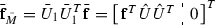
    $$\begin{aligned} \bar{V}^T={\bar{F}_{\bar{\mathbf{w}}_1}\over \Vert \hat{U}_2\hat{U}_2^T\mathbf{f}\Vert +1}\cdot \left[ \begin{array}{c} \hat{U}_2\hat{U}_2\mathbf{f}~\\ 1 \end{array}\right] + \left[ \begin{array}{cc} ~\hat{U}_2~~ &{} 0~\\ 0~ &{} 1~ \end{array}\right] \cdot \bar{{\varvec{\varphi }}}'+\left[ \begin{array}{c} \bar{{\varvec{\tau }}}_1 \\ 0 \end{array}\right] , \end{aligned}$$

    (27)

    where both $\bar{\mathbf{w}}_1,~\bar{{\varvec{\tau }}}_1\in \mathbb {R}^{ n}$ and reside in ${\mathcal {R}}(BR^{-1}B^T)$, the SVD of $(BR^{-1}B^T)$ is $\hat{U}\hat{\varSigma }\hat{U}^T$, , $\hat{U}_2\in \mathbb {R}^{{ n}\times ({ n}-\hat{{ r}}+1)}$, $\hat{U}_1\in \mathbb {R}^{{ n}\times \hat{{ r}}}$, $\hat{\varSigma }=\text{ diag }(\hat{\varSigma }_1,0)\in \mathbb {R}^{{ n}\times { n}}$, $\hat{\varSigma }_1\in \mathbb {R}^{\hat{{ r}}\times \hat{{ r}}}$, $\bar{{\varvec{\varphi }}}'\in \mathbb {R}^{{ n}-\hat{{ r}}+1}$, , and the CQF $\bar{F}_{\bar{\mathbf{w}}_1}: {\mathcal {R}}(BR^{-1}B^T)\subseteq \mathbb {R}^{ n}\rightarrow \mathbb {R}$,

    $$\begin{aligned} \bar{F}_{\bar{\mathbf{w}}_1}(\bar{\mathbf{w}}_1)=\bar{\mathbf{w}}_1^TBR^{-1}B^T\bar{\mathbf{w}}_1/2-\mathbf{f}^T\hat{U}_1\hat{U}_1^T\bar{\mathbf{w}}_1-L/2. \end{aligned}$$

    (28)

Proof

See “Appendix C”.$\square$

Remark 4.2

In Sects. 4.1 and 4.2, the systems under consideration are quadratic in the control input, while the performance index also allows the general (non-quadratic) dependence on the system state [6], as represented by $L(\mathbf{x})$ in Eqs. (10) and (22). Note that, given the quadratic-in-control performance index, the associated HJE, HJBE, and HJI are thus quadratic in the unknown variable: the gradient of the performance index, respectively. In addition, till this stage for optimality recovery, there exists no solving of any PDE. The remaining issue is how to extract the optimal element (that is, the value function V or $\hat{V}$) that satisfies the curl condition [11, 12], among all candidates as parameterized by Eqs. (15), (18)–(20), and (25)–(28), respectively. Aiming at this research direction, [6] pioneers by connecting with the SDRE scheme, and Sect. 4.3 provides further preliminary analyses.

4.3 Relating to the Optimality Using SDRE/SDDRE

In the field of nonlinear optimal control, the SDRE (resp., SDDRE) scheme deals with the infinite (resp., finite)-time horizon, considering the value function $V(\mathbf{x})$ in Eq. (10) (resp., $\hat{V}(\mathbf{x},t_f)$ in (22)). Recent literature toward this research direction includes [28], with an intention of mutual conversation for the common good [23]. To remain focused in this presentation, we reference the survey [11] for a general picture of the scheme, while the main result of this subsection (Theorem 4.2) gives a preliminary to the optimality recovery, as based on or motivated by more recent findings that, for example, preliminarily and analytically clarify/guarantee the property of global asymptotic stability using SDRE [18, 19]. From a different viewpoint, Theorem 4.2 also provides a more efficient approach for a specific consideration instead in [20, Sects. 5.2 and 5.3], as discussed in [20, Remark 5.7].

Theorem 4.2

(A Parameterization of ${\varvec{\xi }}_\perp$)

Consider any ${\varvec{\xi }}\in \mathbb {R}^{ n}$ with $\Vert {\varvec{\xi }}\Vert =1$. Let be orthogonal. The flexibility of the last $({ n}-1)$ columns of $\bar{\varXi }$ can be parameterized by

(29)

where $Y\in \mathbb {R}^{({ n}-1)\times ({ n}-1)}$ is orthogonal, $H_{\varvec{\iota }}{:}{=} I_{ n}-2{\varvec{\iota }}{\varvec{\iota }}^T\in \mathbb {R}^{{ n}\times { n}}$, and ${\varvec{\iota }}\in \mathbb {R}^{ n}$, ${\varvec{\iota }}{:}{=}({\varvec{\xi }}-\mathbf{e}_1)/\Vert {\varvec{\xi }}-\mathbf{e}_1\Vert$, if $~{\varvec{\xi }}\ne \mathbf{e}_1$; $\mathbf{0}$, otherwise.

Proof

Consider the case of ${\varvec{\xi }}\ne \mathbf{e}_1$, while the other case follows similarly. The derivations largely rely on the selected Householder reflection ($H_{\varvec{\iota }}$) [24]. The design concept is to construct a reflection from ${\varvec{\xi }}$ to, representatively, $\mathbf{e}_1$. Consider the (symmetric and orthogonal) Householder matrix in Eq. (29), more explicitly,

$$\begin{aligned} H_{\varvec{\iota }}=I_{ n}-(2/\Vert {\varvec{\xi }}-\mathbf{e}_1\Vert ^2)\cdot ({\varvec{\xi }}{\varvec{\xi }}^T-{\varvec{\xi }}\mathbf{e}_1^T-\mathbf{e}_1{\varvec{\xi }}^T+\mathbf{e}_1\mathbf{e}_1^T ), \end{aligned}$$

then we have $H_{\varvec{\iota }}\cdot {\varvec{\xi }}=\mathbf{e}_1$ and $\mathbf{e}_1^T\cdot (H_{\varvec{\iota }}\cdot {\varvec{\xi }}_\perp ^T)=\mathbf{0}^T$, where the latter is owing to the property that the inner product is preserved under multiplication by an orthogonal matrix. Moreover, $H_{\varvec{\iota }}\cdot \bar{\varXi }=\text{ diag }(1,Y)$, where Y is specified in (29) and, by virtue of $H_{\varvec{\iota }}=H_{\varvec{\iota }}^{-1}=H_{\varvec{\iota }}^T$, it is equivalent to $\bar{\varXi }=H_{\varvec{\iota }}\cdot \text{ diag }(1,Y)$. Extracting the last $({ n}-1)$ columns of yields the result. $\square$

Remark 4.3

Take the planar case as an example, ${\varvec{\xi }}=[\xi _1,\xi _2]^T$, then we have the following specialized results that are consistent with the literature [19, 23]: (A) If ${\varvec{\xi }}\ne \mathbf{e}_1\Leftrightarrow \xi _1\ne 1$, then $\xi _2\ne 0$, while $H_{\varvec{\iota }}{\varvec{\xi }}_\perp ^T=\mathbf{e}_2\Leftrightarrow {\varvec{\xi }}_\perp ^T=H_{\varvec{\iota }}\cdot \mathbf{e}_2=[\xi _2,-\xi _1]^T$; and (B) If ${\varvec{\xi }}=\mathbf{e}_1$, then $H_{\varvec{\iota }}=I_2$, while ${\varvec{\xi }}_\perp ^T=\mathbf{e}_2$.

Remark 4.4

Practically speaking, MATLAB$^{\textregistered }$ computes an example of ${\varvec{\xi }}_\perp ^T$ using the command “null(${\varvec{\xi }}'$)”, which is implemented by performing the SVD on

In the literature, there exist a diversity of algorithms to compute the SVD, notably Golub–Reinsch SVD and R-SVD [29]. Note that it is excessive to compute the full SVD but, actually, sufficient till that all the right singular vectors of the matrix ‘${\varvec{\xi }}^T$’ are obtained. According to [29], the former iterative SVD algorithm requires operation counts $8{ n}^3+4{ n}^2$ to compute an example of ${\varvec{\xi }}_\perp$, whereas $11{ n}^3+2{ n}^2$ for the latter. As an alternative, Theorem 4.2 algebraically and more efficiently solves this issue, through simple calculations in computing the last $({ n}-1)$ columns of $H_{\varvec{\iota }}$ in Eq. (29), where $Y=I_{{ n}-1}$ adopts a simple choice.

5 A Benchmark Example

Consider an ITHNOC regulation problem that is of benchmark importance [11], while in the form of System (9) and Performance Index (10), where ${ n}=2$, $p=1$, $\mathbf{f}=[x_2,-x_1e^{x_1}+x_2^2/2]^T$, $\mathbf{b}=[0,e^{x_1}]^T$, $L=2x_2^2$, and $r=2$ [27]. Note that we also conform the setting in the earlier [27] to System (9) that is in accordance with [11], except normalizing the index (with respect to “$L=x_2^2$ and $r=1$”). This leads to the same conclusion of and consistency by this demonstration, but in a more cogent manner, since the following derivations involve many arithmetic multiplications and divisions. The objective is to regulate any nonzero initial state to the equilibrium at the origin. In this regard, the optimal controller (12) has been explicitly shown as $u_\mathrm{opt}^\infty =-x_2$, with the associated $V_\mathbf{x}=[2x_1-x_2^2e^{-x_1},~2x_2e^{-x_1}]$. This example demonstrates the results in Theorems 3.1, 3.2, Corollary 4.1, and Fig. 1.

For easy comparison, the following parameter values are summarized:

• (i) $\mathbf{b}\mathbf{b}^T/r=\text{ diag }(0,e^{2x_1}/2)$;

• (ii) rank$(\mathbf{b}\mathbf{b}^T/r)=1$;

• (iii) the SVD of $(\mathbf{b}\mathbf{b}^T/r)$ is

  

  where $U_1=[0,1]^T$, $U_2=[1,0]^T$, and $\varSigma _1=e^{2x_1}/2$;

• (iv) $(\mathbf{b}\mathbf{b}^T/r)^\dagger =\text{ diag }(0,2e^{-2x_1})$ and its square root $(\mathbf{b}\mathbf{b}^T/r)^{\dagger /2}=\text{ diag }(0,\sqrt{2}e^{-x_1})$;

• (v) $\mathbf{f}=\mathbf{f}_M+\mathbf{f}_{M^\perp }$, where $\mathbf{f}_M\in {\mathcal {R}}(M)$, $\mathbf{f}_M=U_1U_1^T\mathbf{f}=[0,x_2^2/2-x_1e^{x_1}]^T$, while $\mathbf{f}_{M^\perp }=U_2U_2^T\mathbf{f}=[x_2,0]^T\in {\mathcal {R}}(M)^\perp$.

Since rank$(\mathbf{b}\mathbf{b}^T/r)<n$, which is rank-deficient, we apply (B) of Corollary 4.1. Moreover, given that $\mathbf{f}\in {\mathcal {R}}(\mathbf{b}\mathbf{b}^T/r)\Leftrightarrow x_2=0$, divide the discussions into whether $x_2=0$, respectively as, (a) and (b) below.

• (a) $x_2=0$ ($\mathbf{f}\in {\mathcal {R}}(\mathbf{b}\mathbf{b}^T/r))$. In this case, the solvability condition in Eq. (16) is satisfied since $\mathbf{f}^T(\mathbf{b}\mathbf{b}^T/r)^\dagger \mathbf{f}+L=2x_1^2>0$. By (Ba) in Corollary 4.1, the solution set of HJE–CQE (13) is given by Eq. (18), that is,

  $$\begin{aligned} \mathbf{z}= & {} \sqrt{2x_1^2}\cdot \text{ diag }(0,\sqrt{2}e^{-x_1})\cdot \tilde{\varvec{\rho }}+\tilde{\varvec{\varepsilon }}+\text{ diag }(0,2e^{-2x_1})\cdot \left[ 0,-x_1e^{x_1}\right] ^T\\= & {} [~\tilde{\varvec{\varepsilon }}_1,~2|x_1|e^{-x_1}\tilde{\varvec{\rho }}_2-2x_1e^{-x_1}~]^T, \end{aligned}$$

  where $\tilde{\varvec{\rho }}=[0,\tilde{\varvec{\rho }}_2]^T\in \mathbb {R}^2$, $\tilde{\varvec{\rho }}_2=\pm 1$, since $\tilde{\varvec{\rho }}\in {\mathcal {R}}(\mathbf{b}\mathbf{b}^T/r)={\mathcal {R}}([0,1]^T)$, while $\tilde{\varvec{\varepsilon }}=[\tilde{\varvec{\varepsilon }}_1,0]^T\in \mathbb {R}^2$, $\tilde{\varvec{\varepsilon }}_1\in \mathbb {R}$, since ${\tilde{\varvec{\epsilon }}}\in {\mathcal {N}}(\mathbf{b}\mathbf{b}^T/r)={\mathcal {R}}([1,0]^T)$. In agreement with Corollary 4.1 and Theorem 3.1, the gradient of the value function that solves the HJE–CQE (13), $V_\mathbf{x}=[2x_1,0]$ in this case, is included in the solution set, which is by specifically while uniquely assigning the parameters $\tilde{\varvec{\varepsilon }}_1=2x_1$ and $\tilde{\varvec{\rho }}_2=\mathrm {sgn}(x_1)$. Also, the spanning vectors $\tilde{\varvec{\varepsilon }}$ and $\tilde{\varvec{\rho }}$ are orthogonal to each other, and the parameter-solution mapping ${\mathcal {Z}}_{1\mathbf{f}}^2\rightarrow \varOmega _{1\mathbf{f}}^2$ is a bijection, where

  $$\begin{aligned}&{\mathcal {Z}}_{1\mathbf{f}}^2{:}{=} \big \{\mathbf{z}\in \mathbb {R}^2:\hbox {HJE}{-}\hbox {CQE}~(13),~\mathbf{f}^T(\mathbf{b}\mathbf{b}^T/r)^\dagger \mathbf{f}+L>0,\text{ and }~\mathbf{f}\in { {\mathcal {R}}(\mathbf{b}\mathbf{b}^T/r)}\big \},\\&\varOmega _{1\mathbf{f}}^2{:}{=} \{(\tilde{\varvec{\rho }},\tilde{\varvec{\epsilon }})\in \mathbb {R}^2\times \mathbb {R}^2:\tilde{\varvec{\rho }}\in {{\mathcal {R}}(\mathbf{b}\mathbf{b}^T/r)},~{\Vert \tilde{\varvec{\rho }}\Vert }={1},~\mathrm{and}\,\,{\tilde{\varvec{\epsilon }}}\in { {\mathcal {R}}(\mathbf{b}\mathbf{b}^T/r)}^\perp \}.\end{aligned}$$

  This is in accordance with the considered case (B(a)2) in Theorem 3.2 as well as derivations in its proof.

• (b) $x_2\ne 0$ ($\mathbf{f}\not \in {\mathcal {R}}(\mathbf{b}\mathbf{b}^T/r)$). The solvability condition in Eq. (17) is already satisfied. Hence, by (Bb) in Corollary 4.1, the solution set of HJE–CQE (13) is given by Eq. (19):

  $$\begin{aligned} \mathbf{z}=(\tilde{F}_{\tilde{\mathbf{w}}}/x_2^2)\cdot \left[ x_2,0\right] ^T+\left[ 0,\tilde{\varvec{\tau }}_2 \right] ^T, \end{aligned}$$

  (30)

  where $\tilde{\mathbf{w}}=[0,\tilde{\mathbf{w}}_2]^T$, $\tilde{\varvec{\tau }}=[0,\tilde{\varvec{\tau }}_2]^T$, both $\tilde{\mathbf{w}},~\tilde{\varvec{\tau }}\in \mathbb {R}^2$, both $\tilde{\mathbf{w}}_2,~{\varvec{\tau }}_2\in \mathbb {R}$, since both $\tilde{\mathbf{w}},~\tilde{\varvec{\tau }}\in {\mathcal {R}}(\mathbf{b}\mathbf{b}^T/r)={\mathcal {R}}([0,1]^T)$, while for the CQF, $\tilde{\mathbf{w}}\mapsto \tilde{F}_{\tilde{\mathbf{w}}}(\tilde{\mathbf{w}})$,

  $$\begin{aligned} \tilde{F}_{\tilde{\mathbf{w}}}=[e^{2x_1}\tilde{\mathbf{w}}_2^2+2(2x_1e^{x_1}-x_2^2)\tilde{\mathbf{w}}_2-4x_2^2]/4. \end{aligned}$$

  (31)

  Note that the other parameter “the spanning vector $\tilde{\varvec{\varphi }}$” is, and should be, zero. Specifically, by Eq. (46) in the proof for (Bb) of Corollary 4.1, we have

  $$\begin{aligned} \tilde{\varvec{\varphi }}\in {\mathcal {N}}(\mathbf{f}^T)\Leftrightarrow \tilde{\varvec{\varphi }}'\in {\mathcal {N}}(\mathbf{f}^TU_2)={\mathcal {N}}(x_2).\end{aligned}$$

  Given $x_2\ne 0$ in this case, we thus have the unique $\tilde{\varvec{\varphi }}'=0$ and $\tilde{\varvec{\varphi }}=U_2\tilde{\varvec{\varphi }}'=\mathbf{0}\in {\mathcal {N}}(\mathbf{b}\mathbf{b}^T/r)$, respectively. Therefore, in agreement with Corollary 4.1 and Theorem 3.1, the solution set includes the gradient of the value function that solves the HJE–CQE (13), namely

  $$\begin{aligned} V_\mathbf{x}=[2x_1-x_2^2e^{-x_1},~2x_2e^{-x_1}], \end{aligned}$$

  by simple algebraic calculations that easily while uniquely choose

  $$\begin{aligned} \tilde{F}_{\tilde{\mathbf{w}}}^*=2x_1x_2-x_2^3e^{-x_1} \end{aligned}$$

  and $\tilde{\varvec{\tau }}_2^*=2x_2e^{-x_1}$ (denote the corresponding $\tilde{\varvec{\tau }}^*=[0,\tilde{\varvec{\tau }}_2^*]^T$). In addition, the spanning vectors $\mathbf{f}_{M^\perp }$, $\tilde{\varvec{\varphi }}=\mathbf{0}$, and $\tilde{\varvec{\tau }}$ are mutually orthogonal, and the parameter-solution mapping “${\mathcal {Z}}_1\rightarrow \varOmega _1$” is a bijection, where

  $$\begin{aligned} {\mathcal {Z}}_1{:}{=} \{\mathbf{z}\in {\mathbb {R}^2}:\hbox {HJE}{-}\hbox {CQE}~(13)~\text{ and }~\mathbf{f}\not \in {\mathcal {R}}(\mathbf{b}\mathbf{b}^T/r)\} \end{aligned}$$

  and

  $$\begin{aligned} \varOmega _1{:}{=} \{(\tilde{F}_{\tilde{\mathbf{w}}},\tilde{\varvec{\varphi }},\tilde{\varvec{\tau }})\in {\mathbb {R}\times \{\mathbf{0}\}\times \mathbb {R}^2}:\tilde{\varvec{\tau }}\in { {\mathcal {R}}(\mathbf{b}\mathbf{b}^T/r)}~\text{ and }~\tilde{F}_{\tilde{\mathbf{w}}}:{\mathcal {R}}(\mathbf{b}\mathbf{b}^T/r)\rightarrow \mathbb {R}\}. \end{aligned}$$

  It is worth remarking that the flexibility of the solution set in Eq. (30) at the spanning $\tilde{\varvec{\varphi }}$-direction is only the singleton $\{\mathbf{0}\}$, which is consistent with (Bb) of Theorem 3.2.

Finally, we will explicitly determine the unknown variable $\tilde{\mathbf{w}}_2$ (that is, $\tilde{\mathbf{w}}$) in the CQF (31) at the level set value of $\tilde{F}_{\tilde{\mathbf{w}}}^*$, whose effect is coalesced into the solution set in Eq. (30) by way of this CQF. The followings present two approaches: (I) direct calculations using the quadratic formula, which is a special case that also endorses (II) the results in [20, Theorem 5.13 and Remark  5.15].

• (I) Given $\tilde{F}_{\tilde{\mathbf{w}}}^*=2x_1x_2-x_2^3e^{-x_1}$ in Eqs. (30) and (31), it leads to the following equivalent equation:

  $$\begin{aligned} (e^{2x_1}/4x_2)\cdot \tilde{\mathbf{w}}_2^2+[(x_1e^{x_1}-2x_2^2)/x_2]\cdot \tilde{\mathbf{w}}_2+(x_2^2/e^{x_1})-2x_1-x_2=0.~~~~ \end{aligned}$$

  (32)

  Fig. 2

  

  Geometric interpretation of Eqs. (30) and (31).

  The discriminant of this quadratic equation is $(e^{x_1}+x_1e^{x_1}/x_2-x_2/2)^2\ge 0$, and thus, the two solutions are “$2x_2e^{-x_1}$” and “$2x_2^2e^{-2x_1}-2e^{-x_1}(2x_1+x_2)$”. Denote the corresponding solutions, $\tilde{\mathbf{w}}=[0,\tilde{\mathbf{w}}_2]^T$, of the CQF (31) at the level set value of $\tilde{F}_{\tilde{\mathbf{w}}}^*$ as $\tilde{\mathbf{w}}^1$ and $\tilde{\mathbf{w}}^2$, respectively. It is worth emphasizing that the solvability of Eq. (32) can be anticipated, since the “optimality value $\tilde{F}_{\tilde{\mathbf{w}}}^*$” resides in the image of CQF: $\tilde{\mathbf{w}}\mapsto \tilde{F}_{\tilde{\mathbf{w}}}(\tilde{\mathbf{w}})$, according to Eq./Definition (31).

• (II) By virtue of [20, Theorem 5.13] and its application in [20, Remark 5.15], let $M=\mathbf{b}\mathbf{b}^T/(2r)$, $\mathbf{k}_M=-\mathbf{f}_M$, $c=-L/2$, and $\breve{F}_\mathbf{w}=\tilde{F}_{\tilde{\mathbf{w}}}^*$ in [20, Eq. (5.11)], the preimage is parameterized by

  $$\begin{aligned} \tilde{\mathbf{w}}=(\mathbf{b}\mathbf{b}^T/r)^\dagger \mathbf{f}_M+\sqrt{\mathbf{f}_M(\mathbf{b}\mathbf{b}^T/r)^\dagger \mathbf{f}_M+L+2\tilde{F}_{\tilde{\mathbf{w}}}^*}\cdot (\mathbf{b}\mathbf{b}^T/r)^{\dagger /2}\check{\varvec{\rho }},~ \end{aligned}$$

  (33)

  where $\check{\varvec{\rho }}\in {\mathcal {R}}(\mathbf{b}\mathbf{b}^T/r)$ and $\Vert \check{\varvec{\rho }}\Vert =1$. The square root operation in Eq. (33) is consistent since the operand equals $2(x_1-x_2^2e^{-x_1}/2+x_2)^2\ge 0$, which can be expected from [20, (2) of Theorem 5.13]. Additionally, given that the parameter $\check{\varvec{\rho }}\in {\mathcal {R}}(\mathbf{b}\mathbf{b}^T/r)= {\mathcal {R}}([0,1]^T)$ is of unit length, we further denote $\check{\varvec{\rho }}=[0,\check{\varvec{\rho }}_2]^T$, where $\check{\varvec{\rho }}_2=\pm 1$. As a result, while omitting the straightforward but lengthy calculations for brevity, all/both the solutions in Eq. (33) are exactly the same as that through direct calculations (I), namely, $\tilde{\mathbf{w}}^1$ and $\tilde{\mathbf{w}}^2$.

To sum up the overall discussions in this case (b), a geometric interpretation is illustrated in Fig. 2, which is a special case of Fig. 1 to this example.

6 Conclusions

From a top-level viewpoint, this article proposes a new method with a major application to nonlinear optimal control, which are within an interconnected framework that further includes potentials in nonlinear/convex optimization.

At first, we present a complete, analytical, necessary and sufficient solvability condition for CQE, as well as the corresponding solutions in closed forms. In other words, this is a general-order extension of the quadratic formula. To be more in-depth, we have also explicitly clarified the bijection between the set of solutions and that of the corresponding parameterization variables. All these results assist in establishing a novel perspective to interpret the relation between CQE and CQF, which facilitates further investigations into its spectrum of applications. Representatively, we apply these results to the following.

In the literature of nonlinear optimal control, this application aligns with a research direction that aims at recovering the optimality. Specifically, regarding both the infinite and finite-time horizons, the gradient of the value function is of great importance. It corresponds to a solution of the formulated CQE that is associated with each of the underlining HJE, HJI, and HJBE. By virtue of the analyses of CQE as above, we are able to formulate an analytical representation of the filtered/concentrated optimality candidates, which is thus ready for the final design stage that takes the curl condition into consideration. Note that, till this stage, all the results and their derivations are algebraic, exact, and involve no computation of any PDE. As inspired by extensive early contributions, we also provide a preliminary result using the SDRE/SDDRE scheme for the remaining stage toward the optimality recovery, which (result) still amounts to a general coverage that, for example, computationally benefits applications beyond. Finally, the proposed results are numerically exemplified through a benchmark ITHNOC problem. The gradient of the value function is indeed captured in the formulated solution set of the corresponding HJE–CQE.

Appendices

Proof of Theorem 3.1 (Solutions of CQE)

Considering the CQE (1), divide the proof into the two cases: (A) M is of full rank and (B) M is rank-deficient.

• (A) If rank$(M)={ n}$, then we have (i) $M^T=M\succ 0$, (ii) M is of full rank and nonsingular, and (iii) the unique square root of M is also symmetric and nonsingular, denoted as $M^{1/2}$ [24]. Therefore, the CQE (1) can be equivalently reformulated as

  $$\begin{aligned}&\mathbf{z}^TM^{1/2}\cdot M^{1/2}\mathbf{z}+\mathbf{k}^TM^{-{1/2}}M^{1/2}\mathbf{z}+c=0\nonumber \\&\Leftrightarrow \left( M^{1/2}\mathbf{z}+M^{-{1/2}}\mathbf{k}/2\right) ^T\left( M^{1/2}\mathbf{z}+M^{-{1/2}}\mathbf{k}/2\right) =\mathbf{k}^TM^{-1}\mathbf{k}/4-c\nonumber \\&\Leftrightarrow \left\| M^{1/2}\mathbf{z}+M^{-{1/2}}\mathbf{k}/2\right\| ^2=\mathbf{k}^TM^{-1}\mathbf{k}/4-c. \end{aligned}$$

  (34)

  Obviously, Eq. (34) is solvable, iff the right-hand side (RHS) is non-negative, as in Condition (2). If the condition is satisfied, that is, CQE (1) is solvable, then further reformulate the consistent Eq. (34) as

  $$\begin{aligned}&\left\| M^{1/2}\mathbf{z}+M^{-{1/2}}\mathbf{k}/2\right\| =\sqrt{\mathbf{k}^TM^{-1}\mathbf{k}/4-c}\\&\Leftrightarrow M^{1/2}\mathbf{z}+M^{-{1/2}}\mathbf{k}/2=\sqrt{\mathbf{k}^TM^{-1}\mathbf{k}/4-c}\cdot \mathbf{v}\text{, } \text{ where } \mathbf{v}\in \mathbb {R}^{ n} \text{ and } \Vert \mathbf{v}\Vert =1,\\&\Leftrightarrow \text{ Eq. } \text{(3) }. \end{aligned}$$

• (B) If rank$(M)={ r}<{ n}$, let the SVD of M in CQE (1) be given by

  

  (35)

  where $U_1\in \mathbb {R}^{{ n}\times { r}}$, $U_2\in \mathbb {R}^{{ n}\times ({ n-r})}$, $\varSigma _1\in \mathbb {R}^{{ r}\times { r}}$, and $\varSigma _1^T=\varSigma _1\succ 0$. In addition, the following summarize several properties and definitions [22, 24], which are essential in the derivations afterward.

  $$\begin{aligned}&{\mathcal {R}}(M)={\mathcal {R}}(U_1)={\mathcal {R}}(U_1U_1^T)={\mathcal {R}}(U_2)^\perp ={\mathcal {N}}(U_2^T)={\mathcal {N}}(M)^\perp ,\end{aligned}$$

  (36)
  $$\begin{aligned}&{\mathcal {R}}(M)^\perp ={\mathcal {R}}(U_1)^\perp ={\mathcal {R}}(U_2)={\mathcal {R}}(U_2U_2^T)={\mathcal {N}}(U_1^T)={\mathcal {N}}(M),\end{aligned}$$

  (37)
  $$\begin{aligned}&M^\dagger {:}{=} U_1\varSigma _1^{-1}U_1^T,\end{aligned}$$

  (38)
  $$\begin{aligned}&M^{\dagger /2}{:}{=} U_1\varSigma _1^{-{1/2}}U_1^T, \end{aligned}$$

  (39)

  where both $M^\dagger$ and $M^{\dagger /2}$ are uniquely determined. Perform the equivalence transformation with respect to the U-basis, where is orthogonal:

  $$\begin{aligned} \mathbf{z}= & {} U_1\mathbf{z}_1+U_2\mathbf{z}_2,\end{aligned}$$

  (40)
  $$\begin{aligned} \mathbf{k}= & {} \mathbf{k}_M+\mathbf{k}_{M^\perp }\nonumber \\= & {} U_1\mathbf{k}_1+U_2\mathbf{k}_2, \end{aligned}$$

  (41)

  where $\mathbf{z}_1=U_1^T\mathbf{z}\in \mathbb {R}^{ r}$, $\mathbf{z}_2=U_2^T\mathbf{z}\in \mathbb {R}^{ n-r}$, $\mathbf{k}_1=U_1^T\mathbf{k}\in \mathbb {R}^{ r}$, $\mathbf{k}_2=U_2^T\mathbf{k}\in \mathbb {R}^{ n-r}$, $\mathbf{k}_M=U_1\mathbf{k}_1\in {\mathcal {R}}(M)$, $\mathbf{k}_{M^\perp }=U_2\mathbf{k}_2\in {\mathcal {R}}(M)^\perp$, and both $\mathbf{k}_M,~\mathbf{k}_{M^\perp }\in \mathbb {R}^{ n}$. Because U is orthogonal, we have $I_{ n}=UU^T=U_1U_1^T+U_2U_2^T$ and, by Eqs. (40) and (41), we can reformulate the CQE (1) in terms of the U-basis. More specifically, CQE in Eq. (1) is equivalent to

  $$\begin{aligned}&\mathbf{z}^TU_1\varSigma _1U_1^T\mathbf{z}+\mathbf{k}^T(U_1U_1^T+U_2U_2^T)\mathbf{z}+c=0\nonumber \\&\Leftrightarrow \underbrace{\mathbf{z}_1^T\varSigma _1\mathbf{z}_1+\mathbf{k}_1^T\mathbf{z}_1+c}_{F_{\mathbf{z}_1}:\mathbb {R}^{ r}\rightarrow \mathbb {R}}+\mathbf{k}_2^T\mathbf{z}_2=0, \end{aligned}$$

  (42)

  where $F_{\mathbf{z}_1}$ is (designed to be) a strictly CQF, $\mathbf{z}_1\mapsto F_{\mathbf{z}_1}(\mathbf{z}_1)$, with the positive definite Hessian matrix “$\varSigma _1$”. Therefore, if $\mathbf{k}_2=\mathbf{0}$, then Eq. (42) is a CQE (the preimage of $F_{\mathbf{z}_1}$ at 0) and, since its Hessian matrix is of full rank that equals “${ n-r}$” and by (A) of this theorem, it is solvable, iff “$\mathbf{k}_2=\mathbf{0}$ and $\mathbf{k}_1^T\varSigma ^{-1}\mathbf{k}_1\ge 4c$”. Otherwise ($\mathbf{k}_2\ne \mathbf{0}$), the $\mathbf{z}_2$-freedom of $\mathbf{z}$ ably contributes to null any element/value in the image of $F_{\mathbf{z}_1}$, such that Eq. (42) is always consistent, that is, solvable. Note that, from Eqs. (36) and (41), we have

  $$\begin{aligned} \mathbf{k}_2=\mathbf{0}\Leftrightarrow U_2^T\mathbf{k}=\mathbf{0}\Leftrightarrow \mathbf{k}\in {\mathcal {R}}(U_1)={\mathcal {R}}(M). \end{aligned}$$

  Therefore, in terms of the original coordinate, the solvability condition CQE (1) is equivalently formulated by Condition (4) or (5). In accordance with the equivalence conditions, respectively, the remaining of this proof is divided into two parts to formulate the corresponding solution sets of CQE (1) or, equivalently, (42) in this case of rank-deficient M.

• (Ba) $\mathbf{k}\in {\mathcal {R}}(M) \text{ and } \mathbf{k}^TM^\dagger \mathbf{k}\ge 4c$ in Condition/Eq. (4)

  In this case ($\mathbf{k}\in {\mathcal {R}}(M)\Leftrightarrow \mathbf{k}_2=\mathbf{0}$), $\mathbf{z}_2\in \mathbb {R}^{ n-r}$ represents a degree of freedom in $\mathbf{z}$, which is of dimension $({ n-r})$ and will be parameterized by the variable ‘${\varvec{\varepsilon }}$’ later in Eq. (44). Moreover, the solution set of CQE (1) (or, equivalently, Eq. (42) when $\mathbf{k}_2=\mathbf{0}$) can be parameterized by (A) of this theorem. Specifically,

  $$\begin{aligned} \mathbf{z}_1=-\varSigma ^{-1}\mathbf{k}_1/2+\sqrt{\mathbf{k}_1\varSigma _1^{-1}\mathbf{k}_1/4-c}\cdot \varSigma _1^{-{1/2}}\cdot {\varvec{\rho }}', \end{aligned}$$

  (43)

  where ${\varvec{\rho }}'$ is a vector of unit length in $\mathbb {R}^{ r}$. The remaining of this derivation is to represent the parameterization (43) in terms of the original coordinate. By Eq. (40), this parameterization (43) is equivalent to

  $$\begin{aligned} U_1^T\mathbf{z}=-\varSigma ^{-1}\mathbf{k}_1/2+\sqrt{\mathbf{k}_1\varSigma _1^{-1}\mathbf{k}_1/4-c}\cdot \varSigma _1^{-{1/2}}\cdot {\varvec{\rho }}', \end{aligned}$$

  which is in the applicable (more explicitly, parameterizable) form using Corollary 3.1, yielding the result:

  $$\begin{aligned} \mathbf{z}=-U_1\varSigma _1^{-1}U_1^T\mathbf{k}/2+{\varvec{\varepsilon }}+\sqrt{\mathbf{k}^TU_1\varSigma _1^{-1}U_1^T\mathbf{k}/4-c}\cdot U_1\varSigma _1^{-{1/2}}U_1^TU_1{\varvec{\rho }}', \end{aligned}$$

  (44)

  where $U_1^TU_1=I_{ r}$ is inserted on purpose for the following derivations, while ${\varvec{\varepsilon }}\in {\mathcal {N}}(M)$, ${\varvec{\varepsilon }}\in \mathbb {R}^{ n}$, parameterizes the $\mathbf{z}_2$-freedom in $\mathbf{z}$ as mentioned above, which is of dimension $({ n-r})$ and so is ${\mathcal {N}}(M)$. Denote ${\varvec{\rho }}=U_1{\varvec{\rho }}'\in {\mathcal {R}}(M)$, a vector of unit length in $\mathbb {R}^{ n}$ since $U_1^TU_1=I_{ r}$. Together with $M^\dagger =U_1\varSigma _1^{-1}U_1^T$ and its unique square root ($M^{\dagger /2}=U_1\varSigma _1^{-{1/2}}U_1^T$) as defined in Eqs. (38) and (39), hence the parameterization (44) can be easily and equivalently formulated as in Eq. (6).

• (Bb) $\mathbf{k}\not \in {\mathcal {R}}(M)$ in Condition/Eq. (5)

  Rewrite Eq. (42) as $\mathbf{k}_2^T\mathbf{z}_2=-(\mathbf{z}_1^T\varSigma _1\mathbf{z}_1+\mathbf{k}_1^T\mathbf{z}_1+c)$, and apply Lemma 3.1 to parameterize the $\mathbf{z}_2$-freedom of $\mathbf{z}$,

  $$\begin{aligned} \mathbf{z}_2=-[(\mathbf{z}_1^T\varSigma _1\mathbf{z}_1+\mathbf{k}_1^T\mathbf{z}_1+c)/\Vert \mathbf{k}_2\Vert ^2]\cdot \mathbf{k}_2+{\varvec{\varphi }}', \end{aligned}$$

  (45)

  where ${\varvec{\varphi }}'\in {\mathcal {N}}(\mathbf{k}_2^T)={\mathcal {N}}(\mathbf{k}^TU_2)$ by Eq. (41), and ${\varvec{\varphi }}'\in \mathbb {R}^{ n-r}$. Note that, from Eqs. (35)–(37) and (41), we can derive the following properties:

  • (i) $\mathbf{z}_1^T\varSigma _1\mathbf{z}_1=\mathbf{z}^TU_1\varSigma _1U_1^T\mathbf{z}=\mathbf{w}^TM\mathbf{w}$, where $\mathbf{w}\in {\mathcal {R}}(M)$, $\mathbf{w}\in \mathbb {R}^{ n}$, represents the $\mathbf{z}_1$-freedom of $\mathbf{z}$;

  • (ii) $\mathbf{k}_1^T\mathbf{z}_1=\mathbf{k}^TU_1U_1^T\mathbf{z}=\mathbf{k}_M^T\mathbf{w}$;

  • (iii) $\Vert \mathbf{k}_2\Vert =\Vert \mathbf{k}_{M^\perp }\Vert$.

  Therefore, given these properties (i)–(iii), we can apply Corollary 3.1 to Eq. (45), which parameterizes the solution set of Eq. (45) or, equivalently, CQE (1) in terms of the original coordinate. Specifically, Eq. (45) is equivalent to

  $$\begin{aligned}&U_2^T\mathbf{z}=-[({\mathbf{z}_1^T\varSigma _1\mathbf{z}_1+\mathbf{k}_1^T\mathbf{z}_1+c)/\Vert \mathbf{k}_2\Vert ^2}]\cdot \mathbf{k}_2+{\varvec{\varphi }}'\nonumber \\&\Leftrightarrow \mathbf{z}=-[({\mathbf{z}_1^T\varSigma _1\mathbf{z}_1+\mathbf{k}_1^T\mathbf{z}_1+c)/\Vert \mathbf{k}_2\Vert ^2}]\cdot (U_2\mathbf{k}_2)+U_2{\varvec{\varphi }}'+{\varvec{\tau }}\nonumber \\&\Leftrightarrow \mathbf{z}=-[({\mathbf{w}^TM\mathbf{w}+\mathbf{k}_M^T\mathbf{w}+c)/\Vert \mathbf{k}_{M^{\perp }}\Vert ^2}]\cdot \mathbf{k}_{M^{\perp }}+{\varvec{\varphi }}+{\varvec{\tau }}, \end{aligned}$$

  (46)

  where both ${\varvec{\tau }},~{\varvec{\varphi }}\in \mathbb {R}^{ n}$, ${\varvec{\tau }}\in {\mathcal {N}}(U_2^T)={\mathcal {R}}(M)$ by Eq. (36), and ${\varvec{\varphi }}=U_2{\varvec{\varphi }}'\in {\mathcal {R}}(U_2)$. As a matter of fact, given (I) ${\mathcal {R}}(U_2)={\mathcal {R}}(M)^\perp ={\mathcal {N}}(M)$ by Eq. (37) and (II)

  $$\begin{aligned} {\varvec{\varphi }}'\in {\mathcal {N}}(\mathbf{k}^TU_2)\Leftrightarrow \mathbf{k}^TU_2{\varvec{\varphi }}'=0\Leftrightarrow \mathbf{k}^T{\varvec{\varphi }}=0\Leftrightarrow {\varvec{\varphi }}\in {\mathcal {N}}(\mathbf{k}^T) \end{aligned}$$

  by Eq. (41), it concludes that ${\varvec{\varphi }}\in {\mathcal {N}}(M)\cap {\mathcal {N}}(\mathbf{k}^T)$. The final step is to further analyze the effect by $\mathbf{w}\in {\mathcal {R}}(M)$, which is formulated as the level sets of the CQF “$F_\mathbf{w}$” in Eq. (8). Specifically, the $\mathbf{z}_1$-freedom of solution $\mathbf{z}$ is coalesced into the coefficient of the vector $\mathbf{k}_{M^\perp }$, while grouped in terms of the level sets of the mapping $F_\mathbf{w}$. Substituting this CQF in Eq./Parameterization (46) yields the result.

Remark A.1

Figure 1 illustrates a geometric interpretation of the parameterization in Eq. (7). In this case of rank-deficient M and $\mathbf{k}\not \in {\mathcal {R}}(M)$, the solution set/space of the CQE (1) is spanned by the three vectors $\mathbf{k}_{M^\perp }$, ${\varvec{\varphi }}$, and ${\varvec{\tau }}$, which are mutually orthogonal. Among the three vectors, only $\mathbf{k}_{M^\perp }$ is fixed/given a priori (solid/black arrow, while ${\varvec{\varphi }}$ and ${\varvec{\tau }}$ as the solid-dotted/black arrows), and the associated solution flexibility along this $\mathbf{k}_{M^\perp }$-direction is in terms of the variable $\mathbf{w}$. As shown in Eq. (42), the effect by $\mathbf{w}\in {\mathcal {R}}(M)$, or the $\mathbf{z}_1$-freedom of $\mathbf{z}$, is grouped into the level sets of CQF $F_{\mathbf{w}}$ (red/dashed line, Eq. (8)), which is exemplified by the number-labeled ellipses. Each level value, respectively, contributes to the coefficient term of the spanning vector $\mathbf{k}_{M^\perp }$, and this effect solely modulates the solution flexibility along this $\mathbf{k}_{M^\perp }$-direction. Similar geometric interpretations apply to the other Parameterizations/Eqs. (3) and (6).

Remark A.2

In this proof of Theorem 3.1, Case (B) of rank-deficient M, the SVD form in Eq. (35) is general. All the derivations do not involve a specific selection of nonunique orthonormal bases for ${\mathcal {R}}(M)$ and ${\mathcal {N}}(M)$, namely the columns of $U_1$ and $U_2$, respectively. This is also reflected in the statements of Theorem 3.1, where, notably, $M^\dagger$ and $M^{\dagger /2}$ [22] are uniquely determined. Besides, since Theorem 3.1 is a cornerstone in this article, all the related results share this property.

Proof of Theorem 3.2 (Bijections in CQE)

The injection is obvious from the proof of Theorem 3.1 (“Appendix A”), and the following derives the surjection, respectively, according to Theorem 3.1.

• (A) (M is of full rank) Regarding Condition (2) and Eq. (3), if $\mathbf{k}^TM^{-1}\mathbf{k}\ne 4c$, then the result follows since $M^{-1}$ is nonsingular, that is, the linear transformation by $M^{-1}$ is one-to-one and onto. Otherwise, the solution is unique ($\mathbf{z}=-M^{-1}\mathbf{k}/2$), and not considered in the former derivation (where $\mathbf{v}\ne \mathbf{0}$).

• (B) (M is rank-deficient)

  • (Ba) (Condition (4)) In Eq. (6), the variable ${\varvec{\rho }}$ is only required to parameterize the case of $\mathbf{k}^TM^{-1}\mathbf{k}=4c$. Accordingly, divide the derivations into the two cases corresponding to the number of required parameterization variables. The case/mapping of (B(a)1) $\varOmega _{{ r}\mathbf{k}}^1\rightarrow {\mathcal {Z}}_{{ r}\mathbf{k}}^1$ (using only one parameterization variable ${\varvec{\epsilon }}$) is straightforward, and thus, we focus on the other one (B(a)2) $\varOmega _{{ r}\mathbf{k}}^2\rightarrow {\mathcal {Z}}_{{ r}\mathbf{k}}^2$. Given the two parameterization variables ${\varvec{\rho }}\in {\mathcal {R}}(M)$ and ${\varvec{\epsilon }}\in {\mathcal {N}}(M)$, the effects by the two variables (to prove the injection) can be decoupled, since ${\varvec{\rho }}$ and ${\varvec{\epsilon }}$ are mutually orthogonal. The following derivations consider the sole effect by ${\varvec{\rho }}$, while that for ${\varvec{\epsilon }}$ is similar but much more straightforward (omitted for brevity). Let both $({\varvec{\rho }}_1,{\varvec{\epsilon }}),~({\varvec{\rho }}_2,{\varvec{\epsilon }})\in \varOmega _{{ r}\mathbf{k}}^2$, where ${\varvec{\rho }}_1\ne {\varvec{\rho }}_2$, with the corresponding solutions/elements in ${\mathcal {Z}}_{{ r}\mathbf{k}}^2$, denoted as $\mathbf{z}_1$ and $\mathbf{z}_2$, respectively. To show the surjection suffices to show that $\mathbf{z}_1\ne \mathbf{z}_2$. Given that

    $$\begin{aligned} \mathbf{z}_1-\mathbf{z}_2=\sqrt{\mathbf{k}^TM^\dagger \mathbf{k}/4-c}\cdot U_1\varSigma _1^{-1/2}U_1^T({\varvec{\rho }}_1-{\varvec{\rho }}_2), \end{aligned}$$

    (47)

    where $M^{-\dagger /2}=U_1\varSigma _1^{-1/2}U_1^T$ is adopted from Eqs. (35) and (39). Notably, the RHS of Eq. (47) includes only operations in the vector space ${\mathcal {R}}(M)$. The vector ${\varvec{\rho }}_1-{\varvec{\rho }}_2\in {\mathcal {R}}(M)$, and $U_1^T({\varvec{\rho }}_1-{\varvec{\rho }}_2)$ gives the coordinates of the vector with respect to the basis $U_1$ for ${\mathcal {R}}(M)$. These coordinates are then multiplied by (nonzero) singular values of M, respectively. After further multiplied by $\sqrt{\mathbf{k}^TM^\dagger \mathbf{k}/4-c}\cdot U_1$, the vector ${\varvec{\rho }}_1-{\varvec{\rho }}_2$ is finally projected, while nonzero-scaled, onto ${\mathcal {R}}(M)\backslash \{\mathbf{0}\}$. This implies $\mathbf{z}_1\ne \mathbf{z}_2$ on the left-hand side of (47) and thus completes the arguments for this case.

  • (Bb) (Condition (5)) In Parameterization (7), the three spanning vectors, $\mathbf{k}_{M^\perp }$, ${\varvec{\varphi }}$, and ${\varvec{\tau }}$, are mutually orthogonal:

    $$\begin{aligned} \left\{ \begin{array}{lll} (\mathbf{k}_{M^\perp })^T{\varvec{\varphi }}=0, &{} \quad \text {since } \mathbf{k}^T{\varvec{\varphi }}=0,\\ {\varvec{\varphi }}^T{\varvec{\tau }}=0, &{}\quad \text {since } M{\varvec{\tau }}=\mathbf{0}\text { and } {\varvec{\tau }}\in {\mathcal {R}}(M),\\ {\varvec{\tau }}^T\mathbf{k}_{M^\perp }=0, &{} \quad \text {since } {\varvec{\tau }}\in {\mathcal {R}}(M) \text { and } \mathbf{k}_{M^\perp }\in {\mathcal {R}}(M)^\perp . \end{array}\right. \end{aligned}$$

    Hence, to prove the injection, the effects by these three parameterization variables/vectors can be decoupled. The remaining derivation is similar to the second half of Case (Ba) as above and thus omitted.

Proof of Theorem 4.1 (Solving HJBE–CQE)

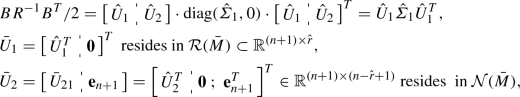
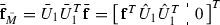
Since rank$(\bar{M})=\hat{{ r}}<{ n}$ and $\bar{\mathbf{f}}\not \in {\mathcal {R}}(\bar{M})$, the HJBE–CQE (24) is always solvable by Condition (5) in Theorem 3.1, where $M=\bar{M}$, $\mathbf{k}=-\bar{\mathbf{f}}$, and the system dimension is (${ n}+1$). Therefore, according to Eqs. (7) and (8) where $\mathbf{z}=\bar{V}^T$, the solution set is parameterized by

$$\begin{aligned} \bar{V}^T=({\bar{F}_{\bar{\mathbf{w}}}/\Vert \bar{\mathbf{f}}_{\bar{M}^\perp }\Vert ^2})\cdot \bar{\mathbf{f}}_{\bar{M}^\perp }+\bar{{\varvec{\varphi }}}+\bar{{\varvec{\tau }}}, \end{aligned}$$

(48)

where all $\bar{\mathbf{w}},~\bar{{\varvec{\varphi }}},~\bar{{\varvec{\tau }}}\in \mathbb {R}^{{ n}+1}$, both $\bar{\mathbf{w}},~\bar{{\varvec{\tau }}}$ reside in ${\mathcal {R}}(\bar{M})$, $\bar{{\varvec{\varphi }}}\in {\mathcal {N}}(\bar{M})\cap {\mathcal {N}}(\bar{\mathbf{f}}^T)$, $\bar{\mathbf{f}}=\bar{\mathbf{f}}_{\bar{M}}+\bar{\mathbf{f}}_{\bar{M}^\perp }$, $\bar{\mathbf{f}}_{\bar{M}}\in {\mathcal {R}}(\bar{M})$, $\bar{\mathbf{f}}_{\bar{M}^\perp }\in {\mathcal {R}}(\bar{M})^\perp$, both $\bar{\mathbf{f}}_{\bar{M}},~\bar{\mathbf{f}}_{\bar{M}^\perp }\in \mathbb {R}^{{ n}+1}$, and the CQF

$$\begin{aligned} \bar{F}_\mathbf{w}(\bar{\mathbf{w}})=\bar{\mathbf{w}}^T\bar{M}\bar{\mathbf{w}}-\bar{\mathbf{f}}_{\bar{M}}^T\bar{\mathbf{w}}-L/2, \end{aligned}$$

(49)

$\bar{F}_{\bar{\mathbf{w}}}: {\mathcal {R}}(\bar{M})\subset \mathbb {R}^{{ n}+1}\rightarrow \mathbb {R}$. Although this suffices a closed-form representation of all the solutions, there is still room for further analytical improvement from a computational perspective. Specifically, the main while remaining part of this proof is to reformulate Eq. (49) into one that only consists of more efficient operations in lower-dimensional spaces. This is viable by exploiting the special structure of HJBE–CQE (24), and thus saves the excessive computational effort.

Note that $\bar{M}$ is rank-deficient, and its rank equals that of its leading principal submatrix of order ${ n}$: $\bar{M}(1:{ n},1:{ n})=BR^{-1}B^T$. Moreover, in accordance with Theorem 3.1 where all cases are categorized first by the rank of the Hessian matrix, we divide the derivations into whether $(BR^{-1}B^T)$ is of full rank or not.

• (A) Rank$(BR^{-1}B^T)={ n}$. Perform the SVD on $\bar{M}$,

  

  (50)

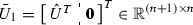
  where $\hat{\varSigma }_1\in \mathbb {R}^{{ n}\times { n}}$ , $\hat{U}\in \mathbb {R}^{{ n}\times { n}}$, , $\eta =\pm 1$, and $\bar{U}_2=\eta \cdot \mathbf{e}_{{ n}+1}$. Notably, the adopted SVD form is unique/general, since $\mathbf{e}_{{ n}+1}$ is (i) the only orthonormal basis for the one-dimensional

  $$\begin{aligned} {\mathcal {N}}(\bar{M})={\mathcal {N}}(\bar{M}^T)={\mathcal {R}}(\mathbf{e}_{{ n}+1}), \end{aligned}$$

  and (ii) the unitary eigenvector associated with the zero eigenvalue (has multiplicity one) of $\bar{M}^T\bar{M}=\bar{M}\bar{M}^T$. In addition, all $\hat{U},~\bar{U}_1,~\bar{U}_2$ are matrices with orthonormal column(s), and $\hat{U}\hat{\varSigma }_1\hat{U}^T$ is the SVD of the submatrix

  $$\begin{aligned} \bar{M}(1:{ n},1:{ n})=(BR^{-1}B^T)/2. \end{aligned}$$

  The following parameter values are computed and summarized for better clarity:

  • (I) and $\bar{\mathbf{f}}_{\bar{M}^\perp }=\bar{U}_2\bar{U}_2^T\bar{\mathbf{f}}=\mathbf{e}_{{ n}+1}$;

  • (II) $\bar{{\varvec{\varphi }}}=\bar{U}_2\bar{{\varvec{\varphi }}}'=\mathbf{0}$ where $\bar{{\varvec{\varphi }}}'\in {\mathcal {N}}(\bar{\mathbf{f}}^T\bar{U}_2)=\{\mathbf{0}\}$, similarly via Eq. (46);

  • (III) denote $\bar{{\varvec{\tau }}}=[\bar{{\varvec{\tau }}}_1^T,0]^T$ and $\bar{\mathbf{w}}=[\bar{\mathbf{w}}_1^T,0]^T$ since both reside in ${\mathcal {R}}(\bar{M})=\mathbb {R}^{ n}\times \{0\}$; and thus

  • (IV) $\bar{\mathbf{w}}\bar{M}\bar{\mathbf{w}}=\bar{\mathbf{w}}_1^TBR^{-1}B^T\bar{\mathbf{w}}_1/2$ and $\bar{\mathbf{f}}_{\bar{M}}^T\bar{\mathbf{w}}=\mathbf{f}^T\bar{\mathbf{w}}_1$.

  Substituting these values in Eqs. (48) and (49), the results are presented more concisely in Eqs. (25) and (26), respectively.

• (B) Rank$(BR^{-1}B^T)=\hat{{ r}}<{ n}$. As mentioned in Remark A.2, the results in Theorem 3.1 are, in particular, independent of the nonuniqueness of the orthonormal bases for ${\mathcal {N}}(M)$, specifically, ${\mathcal {N}}(\bar{M})$ in this case. Therefore, without loss of generality, we choose the following SVD to ease the further analysis on the raw/original solution set in Eq. (48) with (49),

  

  (51)

  where

  

  $\bar{U}_{21}\in \mathbb {R}^{({ n}+1)\times ({ n}-\hat{{ r}})}$, $\hat{\varSigma }_1\in \mathbb {R}^{\hat{{ r}}\times \hat{{ r}}}$, $\hat{U}_1\in \mathbb {R}^{{ n}\times \hat{{ r}}}$, $\hat{U}_1\in {\mathcal {R}}(BR^{-1}B^T)$, $\hat{U}_2\in \mathbb {R}^{{ n}\times ({ n}-\hat{{ r}})}$, and $\hat{U}_2\in {\mathcal {N}}(BR^{-1}B^T)$. Notably, all $\bar{U}_1,~\bar{U}_2,~\bar{U}_{21},~\hat{U}_1,~\hat{U}_2$ are matrices with orthonormal column(s). Moreover, $\mathbf{e}_{{ n}+1}$ (in $\bar{U}_2$) is the selected eigenvector associated with the zero eigenvalue of $\bar{M}^T\bar{M}=\bar{M}\bar{M}^T$. The following parameter values are computed and summarized for better readability:

  • (i) and ;

  • (ii) $\bar{{\varvec{\varphi }}}=\bar{U}_2\bar{{\varvec{\varphi }}}'$ where , similarly according to Eq. (46);

  • (iii) denote $\bar{{\varvec{\tau }}}=[\bar{{\varvec{\tau }}}_1^T,0]^T$ and $\bar{\mathbf{w}}=[\bar{\mathbf{w}}_1^T,0]^T$ since both reside in ${\mathcal {R}}(\bar{M})={\mathcal {R}}(BR^{-1}B^T)\times \{0\}$; and therefore

  • (iv) $\bar{\mathbf{w}}\bar{M}\bar{\mathbf{w}}=\bar{\mathbf{w}}_1^TBR^{-1}B^T\bar{\mathbf{w}}_1/2$ and $\bar{\mathbf{f}}_{\bar{M}}^T\bar{\mathbf{w}}=\mathbf{f}^T\hat{U}_1\hat{U}_1\bar{\mathbf{w}}_1$.

  Substituting these values in Eqs. (48) and (49), the results are presented more concisely in Eqs. (27) and (28), respectively.

References

Rockafellar, R.T.: Convex Analysis. Princeton University Press, Princeton (1970)
Luenberger, D.G., Ye, Y.: Linear and Nonlinear Programming, 2nd and 4th editions. Springer, Switzerland (2016)
Leon, S.J.: Linear Algebra with Applications, 6th edn. Prentice Hall, Upper Saddle River (2002)
Boyd, S., Vandenberghe, L.: Convex Optimization. Cambridge University Press, Cambridge. (23rd/latest printing with corrections, 2018, and its solution manual) (2004)
Patrinos, P., Sarimveis, H.: A new algorithm for solving convex parametric quadratic programs based on graphical derivatives of solution mappings. Automatica 46(9), 1405–1418 (2010)
Won, C.H., Biswas, S.: Optimal control using an algebraic method for control-affine non-linear systems. Int. J. Control 80(9), 1491–1502 (2007)
Yu, J., Jadbabaie, A., Primbs, J., Huang, Y.: Comparison of nonlinear control design techniques on a model of the Caltech ducted fan. Automatica 37(12), 1971–1978 (2001)
Baillieul, J., Samad, T. (eds.): Encyclopedia of Systems and Control. Springer, London (2015)
Raković, S.V., Levine, W.S. (eds.): Handbook of Model Predictive Control. Birkhäuser, Cham (2019)
Kokotović, P., Arcak, M.: Constructive nonlinear control: a historical perspective. Automatica 37(5), 637–662 (2001)
Çimen, T.: Survey of state-dependent Riccati equation in nonlinear optimal feedback control synthesis. J. Guid. Control Dyn. 35(4), 1025–1047 (2012)
Huang, Y., Lu, W.M.: Nonlinear optimal control: alternatives to Hamilton–Jacobi equation. In: 35th IEEE Conference on Decision and Control, pp. 3942–3947 (1996)
Beeler, S.C., Tran, H.T., Banks, H.T.: Feedback control methodologies for nonlinear systems. J. Optim. Theory Appl. 107(1), 1–33 (2000)
Sakamoto, N.: Case studies on the application of the stable manifold approach for nonlinear optimal control design. Automatica 49(2), 568–576 (2013)
Abolvafaei, M., Ganjefar, S.: Maximum power extraction from wind energy system using homotopy singular perturbation and fast terminal sliding mode method. Renew. Energy 148, 611–626 (2020)
Heydari, A., Landers, R.G., Balakrishnan, S.N.: Optimal control approach for turning process planning optimization. IEEE Trans. Control Syst. Technol. 22(4), 1337–1349 (2014)
Ghane, H., Sterk, A.E., Waalkens, H.: Chaotic dynamics from a pseudo-linear system. IMA J. Math. Control Inf. 37(2), 377–394 (2020)
Benner, P., Heiland, J.: Exponential stability and stabilization of extended linearizations via continuous updates of Riccati-based feedback. Int. J. Robust Nonlinear Control 28(4), 1218–1232 (2018)
Lin, L.G., Liang, Y.W., Cheng, L.J.: Control for a class of second-order systems via a state-dependent Riccati equation approach. SIAM J. Control Optim. 56(1), 1–18 (2018)
Lin, L.G., Liang, Y.W., Hsieh, W.Y.: Convex quadratic equations and functions. arXiv:1906.00177
Bemporad, A., Morari, M., Dua, V., Pistikopoulos, E.N.: The explicit linear quadratic regulator for constrained systems. Automatica 38(1), 3–20 (2002)
Urigüen, J.A., Blu, T., Dragotti, P.L.: FRI sampling with arbitrary kernels. IEEE Trans. Signal Process. 61(21), 5310–5323 (2013)
Lin, L.G., Vandewalle, J., Liang, Y.W.: Analytical representation of the state-dependent coefficients in the SDRE/SDDRE scheme for multivariable systems. Automatica 59, 106–111 (2015)
Horn, R.A., Johnson, C.R.: Matrix Analysis, 2nd edn. Cambridge University Press, Cambridge (2013)
Wang, Z., Li, Y.: Nested sparse successive Galerkin approximation for nonlinear optimal control problems. IEEE Control Syst. Lett. 5(2), 511–516 (2021)
Beard, R.W., Saridis, G.N., Wen, J.T.: Galerkin approximations of the generalized Hamilton–Jacobi–Bellman equation. Automatica 33(12), 2159–2177 (1997)
Sznaier, M., Cloutier, J., Hull, R., Jacques, D., Mracek, C.: Receding horizon control Lyapunov function approach to suboptimal regulation of nonlinear systems. J. Guid. Control Dyn. 23(3), 399–405 (2000)
Qin, B., Sun, H., Ma, J., Li, W., Ding, T., Zomaya, A.: Robust \({H}_\infty \) control of doubly fed wind generator via state-dependent Riccati equation technique. IEEE Trans. Power Syst. 34(3), 2390–2400 (2019)
Golub, G.H., Van Loan, C.F.: Matrix Computations, 3rd edn. Johns Hopkins University Press, Baltimore (1996)
Acknowledgements
The authors acknowledge Ivan Birch and Julian Mellor for their assistance in the use of this language, from a native viewpoint; the support from Ministry of Science and Technology, Taiwan, and Max Planck Society, Germany.
Author information
Authors and Affiliations
Corresponding author
Additional information
Communicated by Kok Lay Teo.
Publisher's Note
Springer Nature remains neutral with regard to jurisdictional claims in published maps and institutional affiliations.