


1. Introduction
Climate-induced cryospheric changes such as glacier retreat and decrease in snow cover extent can largely influence the timing, magnitude and distribution of seasonal discharge in the river system (Alford and Armstrong, Reference Alford and Armstrong2010; Immerzeel and others, Reference Immerzeel, Pellicciotti and Bierkens2013; Lutz and others, Reference Lutz, Immerzeel, Shrestha and Bierkens2014; Kayastha and Kayastha, Reference Kayastha, Kayastha, Dimri, Bookhagen, Stoffel and Yasunari2020a; Kayastha and others, Reference Kayastha, Steiner, Kayastha, Mishra and McDonald2020b). The cryospheric regime has been enduring drastic alterations since the last few decades and those changes are mainly associated with increasing temperature (Liu and Chen, Reference Liu and Chen2000; Xu and others, Reference Xu2009; Radić and others, Reference Radić2013; Shea and others, Reference Shea, Immerzeel, Wagnon, Vincent and Bajracharya2015; Bolch and others, Reference Bolch, Wester, Mishra, Mukherji and Shrestha2019). According to Yao and others (Reference Yao2012), the temperature in the Himalayan region has been rising faster than the global average, and this warming is highest between 4800 and 6200 m a.s.l. This elevation range comprises the ablation altitude of almost all Himalayan glaciers in the region. The regional equilibrium line altitudes will shift upward with rising temperatures resulting in the disappearance of debris-free lower elevation glaciers (Mattson and others, Reference Mattson, Gardner, Young and Young1993; Shrestha and Aryal, Reference Shrestha and Aryal2010a; Hassan and others, Reference Hassan2017). Along with challenges associated with water availability and distribution, cryospheric changes can cause potential geohazards such as glacial lake expansion and glacier lake outburst floods, landslides, debris flow, floods and drought (Linglong and others, Reference Linglong, Lide, Jianchen and Pengling2010; Shrestha and others, Reference Shrestha2010b; Bajracharya and others, Reference Bajracharya, Maharjan, Shrestha, Bajracharya and Baidya2014; Donghui and others, Reference Donghui2014).
In central Himalayan basins, a large portion of streamflow contribution comes from monsoon rainfall during the summer season; however, during dry seasons, there is a significant input from snow and ice melt to the river discharge (Wu, Reference Wu2005; Panday and others, Reference Panday, Frey and Ghimire2011; Rajbhandari and others, Reference Rajbhandari, Shrestha, Nepal and Wahid2016). A comprehensive and combined glacier dynamics and glacio-hydrological studies are of utmost importance in this region in order to manage water resources well enough to meet the future water demand of an increasing population, especially during dry seasons. Douglas and others (Reference Douglas, Huss, Swift, Jones and Salerno2016) applied a fully distributed glacio-hydrological model, Glacier-Evolution and Runoff Model (GERM) in the upper Khumbu catchment of the Koshi River basin. GERM was modified to incorporate debris cover using melt reduction factors that vary depending on debris thickness, and to redistribute mass losses according to the observed surface elevation changes. The locally enhanced melt at ice cliffs was also considered in the model to include volume losses. The results from this glacio-hydrological modelling under climate scenarios indicated continued mass losses with a reduction in volume ranging from 60 to 97% by 2100. The runoff was predicted to increase initially followed by an eventual decrease, where runoff in 2100 was predicted to be 8% lower than current levels. A recent study carried out by Xiang and others (Reference Xiang2018) in the Koshi River basin estimated glacial area reduction by 10.4% from 1975 to 2010 at a rate of 0.30% a−1 with increased melting since 2000 (0.47% a−1) using remote-sensing techniques. Donghui and others (Reference Donghui2014) showed similar results using remote-sensing and GIS technologies. They estimated that the glacier area loss in the Koshi River basin during 1976–2009 was 0.59 ± 0.17% a−1, which is one of the fastest reported glacier area losses in the region. The Kangwure Glacier in the Koshi River basin experienced significant mass loss since the 1970s with 34.2% of area loss, 48.2% of ice volume loss and 7.5 m of average thickness decline (Linglong and others, Reference Linglong, Lide, Jianchen and Pengling2010).
The coupled modelling technique has not been applied extensively in the Koshi River basin so there is a considerable knowledge gap in this area of research; however, such method has already been implemented several times in other Himalayan catchments. Wortmann and others (Reference Wortmann, Bolch, Krysanova and Buda2016) integrated glacier dynamics module in the eco-hydrological model SWIM (SWIM-G) to perform glacio-hydrological modelling of the Upper Aksu catchment in the Central Asia with a basin area of 12 991 km2. The model was implemented to estimate ice flow, avalanching processes, snow accumulation and metamorphism as well as glacier ablation with consideration of aspect, debris cover and sublimation. The SWIM-G model was applied with an objective to minimize the gap between semi-distributed, empirical glacio-hydrological models and fully distributed physical models in remote mountainous catchments, where data scarcity is quite common. Ren and others (Reference Ren, Su, Xu, Xie and Kan2018) coupled an energy-balance glacier-melt scheme with the Variable Infiltration Capacity hydrology model (VIC-glacier) and applied the model with 30 m × 30 m grids in a catchment in the Eastern Pamir. Daily maximum and minimum temperature, daily precipitation and daily mean wind speed were provided as input data to the VIC-glacier model. The glacio-hydrological model was validated with field measurements of albedo, energy fluxes, glacier mass balances and discharge. Li and others (Reference Li2019) carried out hydrological projections for the 21st century using Glacier and Snow Melt – WASMOD MODEL (GSM-WASMOD) in the Indian Himalayan Beas Basin up to the Pandoh Dam (upper Beas basin). This model was developed by integrating the water and snow balance modelling system (WASMOD-D) with the GSM module.
This paper examines methods to quantify and assess the cryospheric changes and their influence on downstream hydrological systems. A glacier dynamics model, Open Global Glacier Model (OGGM) (Maussion and others, Reference Maussion2018) is implemented to estimate the future glacier area and volume change until 2100 based on the monthly temperature and precipitation data from the fifth phase of the coupled model intercomparison project – general circulation model (CMIP5-GCM). The future glacier area change obtained from OGGM is incorporated in Glacio-hydrological Degree-day Model (GDM) to simulate the future discharge and contribution from water balance components (snow melt, ice melt, rain and baseflow) to the river discharge in all the sub-basins of the Koshi River basin under RCP 4.5 and 8.5 climate scenarios. GDM can perform with limited data and minimal model parameters, which makes it useful for the Himalayan catchments where the paucity of data is common due to inaccessible terrain and an inadequate number of weather stations.
1.1. Study area
The Koshi River basin is the largest transboundary sub-catchment of the Ganges River basin, which lies in the central Himalaya and covers parts of China, Nepal and India. The Koshi River basin comprises seven sub-basins: Tamor, Arun, Dudhkoshi, Likhu, Tamakoshi, Sunkoshi and Indrawati, respectively, from east to west as shown in Figure 1. In this study, Indrawati is considered as a sub-catchment of the Sunkoshi sub-basin due to the unavailability of discharge data for the Indrawati sub-basin. The Koshi River basin is characterized by steep topography and varying climatic conditions and has five major physiographic regions within Nepal: Terai Plain (<700 m a.s.l.), Siwalik Hills (700–1500 m a.s.l.), Middle Mountains (1500–2700 m a.s.l.), High Mountains (2000–4000 m a.s.l.) and High Himalaya (4000–8848 m a.s.l.) (Shrestha and Aryal, Reference Shrestha and Aryal2010a). The elevation ranges from 113 m a.s.l. in the south to 8848 m a.s.l. in the north, with an associated decreasing temperature trend moving north (Shrestha and others, Reference Shrestha, Wake, Mayewski and Dibb1999). The precipitation is highly heterogeneous in the Koshi River basin due to varying climate and topography, and rainfall is dominated by summer monsoon (June–September) (Chinnasamy and others, Reference Chinnasamy, Bharati, Bhattarai, Khadka and Wahid2015). The total basin area is ~50 000 km2 (for sub-basins considered here). More than 85% of the basin lies above 2000 m a.s.l., with 4.6% covered by clean-ice glaciers and 1% covered by debris-covered glaciers. The glaciers in the Koshi River basin are categorized as temperate summer accumulation type glaciers that are mainly fed by the South Asian summer monsoon (Yao and others, Reference Yao2012; Agarwal and others, Reference Agarwal, Babel and Maskey2014). The summary of the sub-basin information is shown in Table 1. The glacier slope-area distribution shows that 87% of glacier area in the Koshi River basin lies within 0–40⁰ slope and 13% glacier area between 50–70° slope. The glacier aspect-area distribution indicates that 17% of the glacier area is north-facing and 10.3% of the glacier area is south-facing. Altitudinal variation in glacier cover is shown in Figure 2.

Fig. 1. Map showing the sub-basins of the Koshi River basin in the central Himalaya. The red line indicates the Nepalese political boundary, black triangles show hydrological stations, red stars show meteorological stations in Nepal from the Department of Hydrology and Meteorology (DHM), green stars show high altitude meteorological stations in Nepal from EV-K2-CNR, and black stars show meteorological stations in China from the China Meteorological Administration (CMA).

Fig. 2. Glacier area distribution along with elevation in the sub-basins of the Koshi River basin in the central Himalaya.
Table 1. Summary of the sub-basin information for the Koshi River basin

2. Input data
2.1. Observed hydro-meteorological data
The daily discharge data are used from six hydrological stations in all the sub-basins of the Koshi River basin as shown in Table S1. The data were acquired from the Department of Hydrology and Meteorology (DHM) in Nepal. In this study, different time periods are considered for calibration and validation in each sub-basin based on the availability of discharge data. The daily temperature and precipitation data within the Nepalese part of the Koshi River basin are obtained from 21 meteorological stations, among which 19 stations data are provided by DHM and other three stations data are collected from EV-K2-CNR. The three meteorological stations data provided by EV-K2-CNR are located at high altitude (3500–5050 m a.s.l.) within the Dudhkoshi sub-basin. Likewise, daily temperature and precipitation data within the Chinese part of the Koshi River basin are obtained from two meteorological stations maintained and operated by the Chinese Meteorological Administration (CMA). The information on meteorological stations can be found in Table S2. The meteorological stations marked with an asterisk (*) in Table S2 are reference stations for all the sub-basins. In this study, daily temperature and precipitation data of reference stations are provided as input to GDM and the remaining meteorological stations data are used to estimate temperature lapse rate and precipitation gradient. The temperature lapse rate and precipitation gradient values are then used to distribute temperature and precipitation to each grid from reference stations.
2.2. Climate data
The monthly time series of temperature and precipitation from the Climatic Research Unit (CRU) TS v4.01 (Harris and others, Reference Harris, Jones, Osborn and Lister2013) gridded dataset covering the period 1901–2016 are used to calibrate the temperature index model in OGGM (Marzeion and others, Reference Marzeion, Jarosch and Hofer2012). The CRU dataset has a resolution of 0.5⁰ and it is further downscaled to 10′ resolution by assigning the 1961–1990 anomalies to the CRU CL v2.0 gridded climatology (New and others, Reference New, Lister, Hulme and Makin2002). The downscaled CRU dataset has elevation-dependent information which is used to compute the temperature at a given height on the glacier. The gridded monthly temperature and precipitation data of CMCC-CMS GCM from CMIP5 project (Taylor and others, Reference Taylor, Stouffer and Meehl2012) under RCP 4.5 and 8.5 climate scenarios are used in OGGM to simulate future glacier area and volume changes from 2015 to 2100. The low-resolution CMCC-CMS GCM data are downscaled to higher resolution in specific glacier grid points using a statistical downscaling approach, delta or change factor method before estimating glacier dynamics. The Himalayan Adaptation, Water and Resilience (HI-AWARE) climate dataset (Lutz and others, Reference Lutz2016) with 5 × 5 km spatial resolution and daily temporal resolution is provided to GDM to simulate future hydrological conditions under RCP 4.5 and 8.5 climate scenarios from 2021 to 2100. CMCC-CMS GCM is selected among all other GCMs because of its higher combined score for (warm, dry) climate projection as calculated by Lutz and others (Reference Lutz2016) based on the skill score analysis method. Warm, dry situation is the extreme scenario for glacierized catchments and this study is designed to observe future glacio-hydrological conditions under this extreme projection. HI-AWARE dataset is downscaled using statistical approach and bias-corrected using quantile mapping by Lutz and others (Reference Lutz2016).
2.3. Spatial data
The glacier outlines of the Randolph Glacier Inventory (RGI v6.0) (RGI Consortium, 2017), which was released in 2017 and distributed by the Global Land Ice Measurements from Space (GLIMS) are used for initial topographical processing in OGGM. Similarly, the shuttle radar topography mission (SRTM) 90 m digital elevation database v4.1, available from the Consultative Group on International Agricultural Research – Consortium for Spatial Information (CGIAR-CSI) is used in OGGM to project the glacier outline to a local gridded map. The advanced spaceborne thermal emission and reflection radiometer (ASTER) global DEM v2 of 30 m resolution, available from the United States Geological Survey (USGS) is used to compute grid elevation data in GDM. The GlobeLand30 (Jun and others, Reference Jun, Ban and Li2014) land cover map of 30 m resolution is used in GDM. The land cover classes of GlobeLand30 data are merged based on similar topography and surface runoff features to construct six land classes with similar ranges of rainfall runoff coefficient. The six land classes are: land-use type 1 (agricultural land and grassland), land-use type 2 (forest and Shrubland), land-use type 3 (barren land), land-use type 4 (artificial surface and water bodies), clean-ice glacier and debris-covered glacier. The clean-ice glacier and debris-covered glacier outlines of RGI v6.0 are used during land classification. The land cover classification is significant in GDM as it estimates runoff separately for land features such as agricultural land, artificial or urban land and so on. The area covered by land-use types in each sub-basin can be seen in Table 1.
3. Models
The OGGM and GDM are integrated in this study to perform glacier dynamics and glacio-hydrological analyses (Fig. 3). The topographical preprocessing is carried out in OGGM using RGI v6.0 and SRTM DEM data followed by glacier centerline estimation using a geometrical routing algorithm, which is a built-in module in OGGM. The temperature index and ice flow models are then implemented in OGGM for mass-balance and ice thickness estimation. These values are provided as input to the dynamical flowline model to calculate the future glacier area and volume changes based on the CMIP5 GCM dataset. In GDM, ASTER GDEM2 and land-use classes are used to generate grids for each sub-basin. The temperature lapse rate and precipitation gradient distribute temperature and precipitation from the reference stations to each grid and critical temperature differentiates snow and rain from the precipitation. A temperature index model is incorporated in GDM which melts the snow first and then the exposed ice, based on the degree-day factors provided separately for snow, clean-ice and debris-covered ice. The contribution from snow melt, ice melt, rain and baseflow to the river discharge from all grids is routed to estimate total simulated discharge. In order to carry out future discharge simulations, the future glacier area change estimated from OGGM along with the future temperature and precipitation from HI-AWARE climate dataset are provided as input to GDM. The future glacier area change is distributed in grids with glaciated areas for every decade from 2021 to 2100.

Fig. 3. Flowchart showing the workflow involved in OGGM (Maussion and others, Reference Maussion2018) and GDM (Kayastha and Kayastha, Reference Kayastha, Kayastha, Dimri, Bookhagen, Stoffel and Yasunari2020a; Kayastha and others, Reference Kayastha, Steiner, Kayastha, Mishra and McDonald2020b).
3.1. The Open Global Glacier Model (OGGM)
The OGGM is a glacier dynamics and ice flow model which is entirely developed in the Python programming language (Maussion and others, Reference Maussion2018). OGGM is an open-source numerical model framework used for simulating past and future changes in glaciers. OGGM is built based on task-based approaches and these tasks are applied sequentially to either a single (entity task) or set of glaciers (global task). Several workflow processes are involved in OGGM and they are explained in the order in which they are applied for a model run. Figure 4 illustrates a visual representation of OGGM model processes based on an example of the Khumbu Glacier, which lies in the Dudhkoshi sub-basin. The simulations for Khumbu Glacier are carried out in this study based on climate and spatial data described in the input data section.

Fig. 4. The visual representation of workflow processes involved in OGGM with an example based on the Khumbu Glacier: preprocessing (a), Khumbu Glacier flowline (b), Khumbu Glacier catchment area (c), Khumbu Glacier catchment width (d), Khumbu Glacier mass balance (e), Khumbu Glacier ice thickness (f), Khumbu Glacier area (g) and Khumbu Glacier volume (h).
In this model, the glacier outlines are extracted from RGI v6.0 dataset and these outlines are projected onto a local gridded map of the glacier (Fig. 4a). The topographical data or DEM is downloaded in OGGM depending on the glacier's location. OGGM has four default topographical data sources, and for Himalayan catchments, SRTM 90 m DEM is available for download and preprocessing. The DEM is then interpolated to the local grid and this local grid is defined on a Transverse Mercator projection centred over the glacier. The spatial resolution of the DEM depends on the size of the glacier based on the following rule and described in detail by Maussion and others (Reference Maussion2018).

where Δx is the grid spatial resolution (in m), S is the glacier area (in km2) and d 1, d 2 are parameters with values set to 14 and 10, respectively.
A geometrical routing algorithm as described by Kienholz and others (Reference Kienholz, Rich, Arendt and Hock2014) is used to estimate glacier centerlines. First, the terminus of the glacier, or its lowest point, is established along with a series of flowline ‘heads’ (local elevation maxima). The centerlines are then estimated with a least cost routing algorithm minimizing both (i) the total elevation gain and (ii) the distance from the glacier outline. The glacier has a major centerline (the longest one), and tributary branches. The centerlines are further filtered and slightly modified to become glacier flowlines with a regular coordinate spacing (Fig. 4b). Each tributary and the main flowline have their own catchment areas (Fig. 4c), which are computed using a similar flow routing method that is used for estimating the flowlines. Along the flowlines, cross-section widths (Fig. 4d) are obtained by intersecting the normals at each gridpoint with the glacier outlines and the tributaries' catchment areas. The catchment areas are used to correct the cross-section widths so that the flowline of the glacier resembles the actual altitude-area distribution of the glacier.
The mass-balance model used in OGGM is an extended version of the temperature index model presented by Marzeion and others (Reference Marzeion, Jarosch and Hofer2012). The downscaled CRU dataset is used to calibrate the temperature index model. The monthly temperature and precipitation time series are extracted from the nearest CRU CL v2.0 gridpoint for each glacier and then changed to the local temperature using the temperature gradient. The vertical gradient is not applied to precipitation; however, a correction factor (p f) of 2.5 is applied to the original CRU time series similar to Marzeion and others (Reference Marzeion, Jarosch and Hofer2012). In the temperature index model, the monthly mass-balance m i at elevation z is estimated as:

where p f is a global precipitation correction factor, $\;P_{\rm i}^{{\rm Solid}} \;$ is the monthly solid precipitation, T i is the monthly temperature and T Melt is the monthly air temperature above which ice melt is assumed to occur. In this research, 0°C is considered as T Melt. Solid precipitation is calculated as a fraction of the total precipitation: 100% solid if T i ≤ T Solid (0°C), 0% if T i ≥ T Liquid (2°C) and linearly interpolated in between. μ* specifies temperature sensitivity of the glacier and this parameter needs to be calibrated in the temperature index model. The calibration process is first carried out for glaciers whose annual specific mass-balance data are available in the World Glacier Monitoring Service (WGMS) database. The mass-balance calibration process in OGGM is explained in detail by Maussion and others (Reference Maussion2018). The annual specific mass balance of the Khumbu Glacier from 1901 to 2016 is shown in Figure 4e. Based on the estimated mass-balance data and mass conservation laws, an estimate of the ice flux along each glacier cross-section is calculated. Assuming the shape of the cross-section (parabolic or rectangular) and using the principles of ice flow, OGGM estimates the thickness of the glacier along the flowlines (Fig. 4f) and also the total volume of the glacier (Maussion and others, Reference Maussion2018). A dynamical flowline model is used to simulate the advance and retreat of the glacier under preselected climate time series. After estimating the future glacier area (Fig. 4g) and volume (Fig. 4h) for a single glacier within a catchment, results from all single glaciers are compiled to estimate glacier evolution for the whole catchment. This process is carried out for all the sub-basins of the Koshi River basin.
3.2. Glacio-hydrological Degree-day Model (GDM)
The GDM v1.0 is a distributed and gridded glacio-hydrological model that simulates the daily river discharge and estimates contribution from snow melt, ice melt, rain and baseflow to the river discharge (Kayastha and Kayastha, Reference Kayastha, Kayastha, Dimri, Bookhagen, Stoffel and Yasunari2020a; Kayastha and others, Reference Kayastha, Steiner, Kayastha, Mishra and McDonald2020b). The workflow of GDM is presented in Figure 3. GDM is implemented in all the sub-basins of the Koshi River basin with a grid size of 4.04 km2.
The melt module in GDM performs the main algorithm for glacio-hydrological simulation using a temperature index model. The model separately estimates melt for snow, clean ice and ice under debris based on the degree-day approach (Braithwaite and others, Reference Braithwaite and Olesen1989; Kayastha and others, Reference Kayastha, Ageta, Fujita, de Jong, Collins and Ranzi2005) as:

where M is the snow or ice melt in mm d−1 in each grid, T is the daily air temperature in °C and k s, k b and k d are the degree-day factors in mm °C−1 d−1 for snow, clean ice and debris-covered ice, respectively.
The processes and equations governing baseflow simulation module are adopted from soil and water assessment tool (Luo and others, Reference Luo, Arnold, Allen and Chen2012). The baseflow algorithm is based on a two-reservoir system incorporating contribution from shallow and deep aquifers to the river runoff. The surface runoff (QG) encompasses runoff from rain, snow melt and ice melt from each grid as shown in the equation below:

where Q r is the discharge from rain, Q s is the discharge from snow melt and Q i is the discharge from ice melt in m3 s−1. C r and C s are the rain and snow coefficients and Q G is the surface runoff component from each grid in m3 s−1. The total surface runoff contribution Q R from all grids and the total baseflow contribution Q B from all grids are expressed as:


where Q b is the baseflow contribution from each grid and n is the number of grids. The total surface discharge Q R is then routed with the baseflow contribution Q B towards the outlet of the sub-basin through the following equation:

where k is the recession coefficient, Q d is the total discharge in m3 s−1 and d is the d th day. The recession coefficient k is derived by solving Eqn (8), provided by Martinec and Rango (Reference Martinec and Rango1986). The constants x and y calculated from this equation are 0.93 and 0.009, respectively, for all the sub-basins.

GDM is calibrated based on the parameters shown in Table 2. Among these parameters, the positive degree-day factors, snow and rain runoff coefficients and recession coefficients are the key calibration parameters in GDM. The values for positive degree-day factors and critical temperature are derived from the past studies in the central Himalayan catchments (Kayastha and others, Reference Kayastha, Ageta, Fujita, de Jong, Collins and Ranzi2005; Khadka and others, Reference Khadka, Devkota and Kayastha2015). Monthly degree-day factors are provided for lower (<5000 m a.s.l.) and higher (>5000 m a.s.l.) elevations for snow and ice melt. Lower degree-day factors are assigned for lower elevation and higher degree-day factors for higher elevation and likewise, lower degree-day factors are used during monsoon season (June to September) and higher degree-day factors during other months. Similarly, higher values of rain and snow runoff coefficients are allocated during monsoon season compared to other months. The values for land-use runoff coefficients and baseflow parameters are used within the standard range to minimize uncertainty associated with calibration processes. Apart from these parameters, the monthly sunshine hours are needed to estimate potential evapotranspiration using the Thornthwaite equation. The values for possible sunshine hours are derived from the previous studies (Niroula and others, Reference Niroula, Kobayashi and Xu2015).
Table 2. Calibration parameters used in GDM and their respective values

4. Results and discussion
4.1. Glacier area and volume change
A significant loss in glacier area and volume is estimated from 2015 to 2100 in all the sub-basins of the Koshi River basin as shown in Figure 5. The glacier evolution is computed from 2015 to 2100 in this study; however, the future analysis is done from 2021 to 2100 as this time period is used for future discharge simulation using GDM. The glacier outlines used in this study (RGI v6.0) were generated from satellite imagery of around 2015 (RGI Consortium, 2017); therefore, the simulation in OGGM starts from 2015. The average glacier area in the entire Koshi River basin from 2021 to 2100 is estimated to decrease from 2714 to 950 and 407 km2, a 65–85% decrease and the average glacier volume from 203 to 49 and 28 km3, a 76–86% decrease for RCP 4.5 and 8.5 scenarios, respectively. The glacier area and volume decrease rapidly after 2060 and the trend continues until 2100. The reduction in glacier area is more prominent as compared to glacier volume from 2061 to 2100. The major changes in glacier area and volume among all the sub-basins are observed in Likhu sub-basin for both climate scenarios. An 88 and 96% decrease in glacier area and 92 and 97% decrease in glacier volume are observed in Likhu sub-basin for RCP 4.5 and 8.5 scenarios, respectively, from 2021 to 2100 (Table 3). The lowest decrease in glacier area is observed in Dudhkoshi (49%) for RCP 4.5 and in Tamor (69%) for RCP 8.5. The lowest decline in glacier volume is observed in Dudhkoshi, 66 and 77% for RCP 4.5 and 8.5 scenarios, respectively, until the end of the century.

Fig. 5. The glacier area and volume trends from 2015 to 2100 under RCP 4.5 and 8.5 climate scenarios in Tamor (a, b), Arun (c, d), Dudhkoshi (e, f), Likhu (g, h), Tamakoshi (i, j) and Sunkoshi (k, l).
Table 3. Glacier area and volume changes in all the sub-basins of the Koshi River basin under RCP 4.5 and 8.5 scenarios from 2021 to 2100

Huss and Hock (Reference Huss and Hock2018) estimated a glacier volume decrease of 58 ± 13% (RCP 4.5) and 74 ± 11% (RCP 8.5) between 2010 and 2100 in 56 glacierized basins using the Global Glacier Evolution Model (GloGEM). Bolch and others (Reference Bolch, Wester, Mishra, Mukherji and Shrestha2019) projected a decline in glacier volume by up to 90% until 2100 in higher emission pathways and slightly reduced glacier volume percentage in lower emission scenarios in the extended HKH region. Our results are in line with these findings (Table 3). Shea and others (Reference Shea, Immerzeel, Wagnon, Vincent and Bajracharya2015) carried out a similar study in the Dudhkoshi sub-basin to observe changes in the future glacier volume and the results from this research estimated glacier volume reduction between 35 and 62% (RCP 4.5) and between 73 and 96% (RCP 8.5) by 2050 in the Dudhkoshi sub-basin based on the CMIP5 climate data. The findings from our research are in contradiction with the results estimated by Shea and others (Reference Shea, Immerzeel, Wagnon, Vincent and Bajracharya2015). The results from our study have lower values as compared to these findings as our research shows a decrease in glacier area by 13% (RCP 4.5) and 16% (RCP 8.5), and a decrease in glacier volume by 26% (RCP 4.5) and 29% (RCP 8.5) until 2050 in the Dudhkoshi sub-basin. However, based on our results, after 2050, the Dudhkoshi sub-basin is likely to experience a rapid decline in glacier area and volume. From 2050 to 2100, the decline in glacier area is 42% (RCP 4.5) and 85% (RCP 8.5), and the decline in glacier volume is 55% (RCP 4.5) and 68% (RCP 8.5) in the Dudhkoshi sub-basin using OGGM.
4.2. GDM calibration
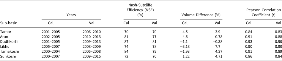
The seasonal pattern of basin streamflow is followed by the simulated discharge during calibration; however, in some of the sub-basins, the model is unable to catch the extreme peaks during high runoff season, which might be due to the underestimation of precipitation in high altitudes. The model is also unable to follow the pattern of observed discharge during the pre-monsoon (March–May) season. The model overestimates discharge during this period and this result can be attributed to the fact that GDM does not use a soil map and therefore, underestimates infiltration and overestimates surface runoff. The calibration and validation graphs for the Dudhkoshi sub-basin are shown below (Figs 6a, c). In general, we can say that GDM is able to represent the overall hydrological dynamics of the Dudhkoshi sub-basin. Similar trends are observed in calibration and validation graphs of remaining sub-basins as well. The statistical analysis for calibration and validation period is carried out using Nash-Sutcliffe Efficiency (NSE), Volume Difference (VD) and Pearson Correlation Coefficient (r). The prediction from models such as GDM is associated with a certain degree of uncertainty due to errors during the calibration of parameters, the design of the model and measurements of input data. In this study, we assume that the model has a higher degree of accuracy and certainty if the NSE index is higher than 0.7 and VD up to ±10%. In all the sub-basins, NSE is estimated ≥70%, VD <10% and r > 0.8 for both calibration and validation periods. The detailed results for all the sub-basins are shown in Table 4. Based on the good performance of model during calibration and validation periods, GDM is considered suitable for future projection analysis.

Fig. 6. The observed and simulated discharge at Rabuwa Bazar hydrological station in the Dudhkoshi sub-basin during calibration (2001–2005) (a) and validation (2009–2013) (c) periods along with precipitation and contribution from water balance components to the river discharge during calibration (b) and validation (d) periods.
Table 4. Nash-Sutcliffe Efficiency (NSE), Volume Difference and Pearson Correlation Coefficient (r) values for all the sub-basins of the Koshi River basin during calibration (cal) and validation (val) periods
Along with the simulated discharge, the contribution from snow melt, ice melt, rain and baseflow to the river discharge during calibration and validation period is also estimated for the baseline period (Figs 6b, d). All discharge components are contributing largely in the peak season (June, July, August and September). There is a significant contribution from snow and ice melt during the pre-monsoon (March, April and May) and post-monsoon (October and November) seasons as well. In monsoon-dominated catchments, such as the Koshi River basin, snow and ice melt contribution plays a significant role in providing water during dry seasons. The highest contribution from snow melt is found in Arun: 21 and 25%, the highest contribution from ice melt in Sunkoshi: 14 and 11%, the highest contribution from rain in Likhu: 41 and 40% and the highest contribution from baseflow in Arun: 52 and 49% for calibration and validation periods, respectively. The lowest contribution from snow melt and ice melt is observed in Likhu for both calibration and validation periods, the lowest contribution from rain in Arun and the lowest contribution from baseflow in Dudhkoshi as shown in Table 5.
Table 5. The mean annual contribution of snow melt, ice melt, rain and baseflow to the river discharge during calibration (cal) and validation (val) periods in all the sub-basins of the Koshi River basin

Gupta and others (Reference Gupta, Kayastha, Ramanathan and Dimri2019) used GDM for calibration and validation of the Tamor sub-basin and estimated snow and ice melt contribution to river discharge as 14.5 and 7.3% for calibration and 12.9 and 10.6% for validation. The findings from our research are in good agreement with the results estimated by Gupta and others (Reference Gupta, Kayastha, Ramanathan and Dimri2019) which can be seen in Table 5. Nepal (Reference Nepal2016) calibrated and validated the J2000 glacio-hydrological model in the Dudhkoshi sub-basin from 2000 to 2010 and estimated a contribution of ~34% from snow and ice melt to the river discharge. The melt runoff contribution was significant during the pre-monsoon season (March to May), providing almost 63% contribution to discharge when water was scarce, compared to 10% during winter (November to February) and ~39% in the monsoon season (June to September). The overland flow contributed ~50% of total discharge, the interflows contributed ~30% and base flow ~20%. The contribution from water balance components to the river discharge in the Dudhkoshi sub-basin is slightly underestimated in our research compared to Nepal (Reference Nepal2016) and this might have occurred due to the differences in melt module and baseflow algorithm in J2000 and GDM.
4.3. Future simulated discharge
The future discharge is simulated using GDM based on the HI-AWARE climate dataset from 2021 to 2100 for RCP 4.5 and 8.5 scenarios. The Koshi River basin is a rainfall-dominated basin where future simulated discharge seems to follow the trend of future precipitation in all the sub-basins. In order to analyse the simulated future discharge, the future time period is separated into two reference periods: 2021–2060 and 2061–2100. Figure 7 shows simulated discharge in all the sub-basins under RCP 4.5 and 8.5 scenarios for two reference time periods. For RCP 4.5 and 8.5 scenarios, the simulated discharge is higher during 2061–2100 compared to 2021–2060, especially for the pre-monsoon and monsoon seasons. The increase in simulated discharge during the monsoon season is due to the increased precipitation in the future. The simulated discharge is lower during 2061–2100 compared to 2021–2060 during the post-monsoon and winter seasons for both RCP 4.5 and 8.5 scenarios. In this research, the glacier area is reduced for every decade based on the results derived from OGGM and glacier area is largely reduced under RCP 8.5 scenario compared to RCP 4.5 scenario; hence, a decrease in simulated discharge is observed during the post-monsoon season mainly for RCP 8.5 scenario after 2060. The winter season has lower simulated discharge due to less rainfall and low contribution from snow and ice melt. The major contribution in the winter season comes from baseflow in all the sub-basins of the Koshi River basin. Gupta and others (Reference Gupta, Kayastha, Ramanathan and Dimri2019) estimated an average decrease in simulated discharge of 0.366 m3 a−1 in the Tamor sub-basin under RCP 4.5 scenario for the period 2021–2050 using GDM based on Coordinated Regional Downscaling Experiment (CORDEX) climate data. However, our study estimates an increase in simulated discharge by 0.0009 m3 a−1 from 2021 to 2050 in Tamor sub-basin for RCP 4.5 scenario based on HI-AWARE dataset. The spatial resolution of CORDEX dataset is coarser (50 km) as compared to HI-AWARE dataset (5 km), which could have caused disparity in the results.

Fig. 7. The monthly average simulated discharge in Tamor (a), Arun (b), Dudhkoshi (c), Likhu (d), Tamakoshi (e) and Sunkoshi (f) sub-basins during two future reference time periods: 2021–2060 and 2061–2100 under RCP 4.5 and RCP 8.5 scenarios compared with the baseline discharge.
The future simulated discharge is increased in all the sub-basins of the Koshi River basin as compared to the baseline period (Fig. 7). This increase in the simulated discharge can be credited to an increase in precipitation in the future. The largest variation is observed in the Likhu sub-basin (Fig. 7d). During the future reference periods, 2021–2060 and 2061–2100, in three sub-basins: Tamor, Arun and Tamakoshi, there is an increase in discharge after 2060 until the end of the century mainly under RCP 8.5 scenario (Table 6). In the Likhu sub-basin, there is no variation after 2060 under RCP 4.5 scenario; however, there is a decrease in discharge under RCP 8.5 scenario. In the Sunkoshi sub-basin, there is a decrease in discharge under RCP 4.5 and no variation under RCP 8.5 scenario after 2060. Nepal (Reference Nepal2016) projected an increase of 13% in the annual discharge by mid-century followed by a slight decrease in the Dudhkoshi sub-basin using J2000 model. Our results from the Dudhkoshi sub-basin indicate an increase of 20% (RCP 4.5) and 23% (RCP 8.5) in the annual discharge from 2021 to 2060 and a small increase in RCP 4.5 and a decrease in 8.5 after 2060 as seen in Table 6.
Table 6. Changes in the future discharge compared to the baseline period in all the sub-basins of the Koshi River basin for future reference periods: 2021–2060 and 2061–2100 under RCP 4.5 and 8.5 scenarios

4.4. Contribution of streamflow components to the future discharge
The contribution of streamflow components to the future discharge is analysed for two future reference periods: 2021–2060 and 2061–2100 under RCP 4.5 and RCP 8.5 scenarios (Table S3). The snow melt contribution is showing a slightly decreasing trend after 2060, which is reasonable considering the fact that snow-covered area and snow storage capacity decrease with increasing temperature, hence, decreased snow melt in the future. The increase in temperature moves the snowline altitude higher, further decreasing the contribution from snow melt. In the Tamor sub-basin, the snow melt contribution is constant with a slight increase from 2061 to 2100 under RCP 8.5 scenario. In all the sub-basins, a significant contribution from snow melt to the discharge during the monsoon (June to September) and post-monsoon (October and November) seasons is observed from 2021 to 2100 for both RCP 4.5 and 8.5 scenarios (Figs 8a, b). The snow melt contribution is higher in the Arun sub-basin compared to the other sub-basins. Likewise, there is also a considerable amount of contribution seen during the pre-monsoon (March to May) season. The highest snow melt contribution during the pre-monsoon season is observed in the Dudhkoshi sub-basin and the highest contribution in the post-monsoon season is observed in Arun for both RCP 4.5 and 8.5 scenarios. The ice melt contribution is observed higher in Dudhkoshi during the pre-monsoon season and higher in Arun during the post-monsoon season for both RCP 4.5 and 8.5 scenarios. The ice melt contribution in Sunkoshi seems to be decreasing in RCP 8.5 scenario compared to RCP 4.5 in almost all the seasons and it might be due to the large reduction in glacier area in the basin for RCP 8.5 scenario. It should be noted that despite a substantial decrease in glacier area in all the sub-basins, there is still a significant contribution from ice melt in the future, which signifies rapid melting in the sub-basins that could result in a complete disappearance of glaciers especially in smaller glacierized basin such as Likhu. Gupta and others (Reference Gupta, Kayastha, Ramanathan and Dimri2019) estimated increased glacial melt from 2021 to 2050 using GDM based on CORDEX climate data which support the outcomes of this research. Rain and baseflow contribution showed fluctuating trends within the two future reference periods, which could be related to the fluctuating trend of precipitation in the sub-basins. Based on RCP 4.5 and 8.5 scenarios, it can be said that there will be a significant contribution from rain and baseflow in the future which could partially compensate for decreased discharge contribution of snow melt in the basin.
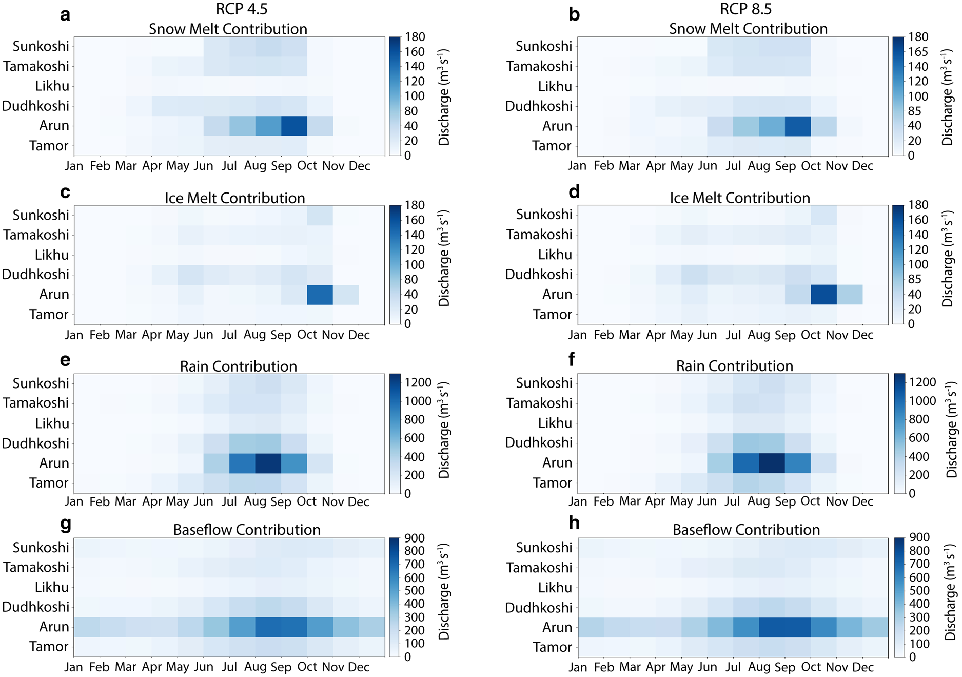
Fig. 8. The monthly contribution from snow melt (a, b), ice melt (c, d), rain (e, f) and baseflow (g, h) to the river discharge from 2021 to 2100 under RCP 4.5 and 8.5 scenarios in all the sub-basins of the Koshi River basin.
5. Uncertainty and sensitivity analyses
The glacio-hydrological model (GDM) used in this research does not process gridded meteorological data and the use of temperature lapse rate and precipitation gradient can considerably affect the spatial distribution of temperature and precipitation in grids, and hence, the model output. The spatial distribution of precipitation is particularly more central in this research due to the topographical and climatological variation in Nepalese and Chinese regions of the sub-basins. In order to minimize the effects of this limitation on the model output, all available meteorological stations data from the entire Koshi River basin are used in this research. However, the number of meteorological stations within the Koshi River basin is still very limited and long-term data are not available for most of the stations. The quality and paucity of meteorological input data are considerable sources of uncertainty. In this particular research, there is no available station with both temperature and precipitation data within the Likhu sub-basin, which is the smallest sub-basin with an area of 850 km2 and therefore, the reference station is selected from the nearest sub-basin. Similarly, for the Arun sub-basin, which is the largest sub-basin with an area of 33 396 km2, the available meteorological stations data from both China and Nepal are not enough for the estimation of temperature lapse rate and precipitation gradient leading to uncertainty during the distribution of input data to each grid. Moreover, for future projection, uncertainty mainly arises from GCM and RCM climate data. In this study, high-resolution climate data are used to minimize the uncertainty; however, these data are downscaled using statistical approach or delta method and such approach can lead to higher uncertainties compared to dynamical downscaling methods. In the delta method (Trzaska and Schnarr, Reference Trzaska and Schnarr2014), a ‘change factor’ is used as the ratio between GCM simulations of future and current climate and it is further applied as a multiplicative factor to compute the future regional climate. The same ratio is applied to all the regions lying within the same GCM gridpoint, and hence, the local differences in future climate due to the local features are not considered unlike dynamical downscaling approaches. Despite its shortcomings, the statistical approach is still one of the most applied methods in the Himalayan catchments as minimal data and low computational resources are required for downscaling. The uncertainty associated with the climate data can also be minimized by providing multiple GCMs ensemble data; however, in this study, only one GCM dataset is used and downscaled for future projections in both glacier dynamics and glacio-hydrological modelling. The detailed analysis of uncertainty assessment in glacio-hydrological modelling has been carried out extensively in the past studies (Huss and others, Reference Huss, Zemp, Joerg and Salzmann2013; Ragettli and others, Reference Ragettli, Pellicciotti, Bordoy and Immerzeel2013; Zhang and others, Reference Zhang, Su, Yang, Hao and Tong2013).
The quantitative assessment of uncertainties associated with the input data and model processes is complex; therefore, a sensitivity analysis has been carried out to understand the sensitivity of model parameters and input data to the model outputs. The degree-day factors have been changed by ±1 mm °C−1 d−1 and ±2 mm °C−1 d−1, temperature lapse rate by ±0.1°C 100 m−1 and ±0.2°C 100 m−1 and precipitation gradient by ±10% and ±20% as shown in Figure 9. The estimated discharge from the sensitivity analysis is compared with the simulated discharge from the baseline period and the change in percentage is calculated. Based on this analysis, the model output is less sensitive to degree-day factors for both ice (k b and k d) and snow (k s) as compared to the temperature lapse rate and the precipitation gradient in all the sub-basins. The discharge variation is slightly higher in the Arun sub-basin for degree-day factors than rest of the sub-basins and this result can be attributed to the higher glacier area in the Arun sub-basin. The Koshi River basin is a rainfall-dominated and monsoon-fed catchment; therefore, change in precipitation gradient is expected to have more influence in the river discharge. However, the results from sensitivity analysis depict that the model is more sensitive to the temperature lapse rate than the precipitation gradient. This may be because the temperature-dependent melt module in GDM largely governs the melt processes and water balance estimation. The lower value of temperature lapse rate means higher temperature in the higher elevation, and hence, increased ice melt and increased river discharge. The temperature lapse rate is particularly more significant in sub-basins such as Arun, Tamakoshi and Sunkoshi. These three sub-basins have one thing in common, they all have a substantial portion of their areas in arid climatic regions of the Himalaya that receive very less rainfall throughout the year. The Arun sub-basin is considerably sensitive to precipitation gradient as well and it can be said that the larger basin area of the Arun sub-basin makes it more sensitive to most of the model parameters as compared to the other sub-basins. The Likhu sub-basin is also quite sensitive to change in the precipitation gradient. When precipitation gradient is increased by 20%, the discharge increased by 27% in the Likhu sub-basin. This sensitivity to precipitation gradient justifies the considerable difference between baseline and future simulated discharge in the Likhu sub-basin. Similarly, the Sunkoshi sub-basin seems to be the least sensitive to the precipitation gradient among all the sub-basins and this explains the minimum difference between the baseline and the future simulated discharge in the Sunkoshi sub-basin.

Fig. 9. GDM sensitivity to the parameters; degree-day factor for clean and debris-covered ice (k b and k d) (a), degree-day factor for snow (k s) (b), temperature lapse rate (c) and precipitation gradient (d).
6. Conclusion
This paper has examined the coupled modelling technique in the Himalayan catchment and synthesized cryospheric and hydrologic change projections in response to the climate change. The results from this research demonstrate prominent changes in the cryospheric and hydrologic regimes. Such changes can have dire consequences on the livelihood of thousands of people living in the catchment. Based on the glacier dynamics simulations in this study, the average glacier area in the Koshi River basin from 2021 to 2100 is estimated to decrease from 2714 to 950 and 407 km2, a 65–85% decrease and the average glacier volume from 203 to 49 and 28 km3, a 76–86% decrease for RCP 4.5 and 8.5 scenarios, respectively. These results from the glacier dynamics model are incorporated into a glacio-hydrological model to simulate future hydrologic conditions. The future simulated discharge is higher in all the sub-basins compared to the baseline period; however, this increase is considerably larger in the sub-basins like Likhu, Arun and Dudhkoshi. Moreover, in future, increased discharge is observed in the pre-monsoon and monsoon seasons and decreased discharge in the post-monsoon and winter seasons. This trend is more significant after 2060, which can lead to wetter wet seasons and drier dry seasons in the far future. The snow melt contribution shows a decreasing trend after 2060, which is reasonable considering the fact that snowfall amount will decrease and rainfall will increase with increasing temperature; hence, decreased snow melt in the future. Furthermore, it should be noted that despite a colossal decrease in the glacier area in all the sub-basins, there is still a significant contribution from ice melt in the future, which signifies rapid melting in the sub-basins that can result into the disappearance of glaciers, especially in smaller glacierized basin such as Likhu. In both RCP 4.5 and 8.5 scenarios, there is a significant contribution from rain and baseflow in the future, which can compensate for decreased discharge contribution of snow melt in the basin. Similarly, based on the sensitivity analysis of the GDM parameters, the model output is more sensitive to the temperature lapse rate as compared to the precipitation gradient and the degree-day factor, which is primarily due to a larger significance of the temperature-dependent melt module in GDM. The findings of this research are vital in improving our understanding of coupled modelling approach along with the localized future cryospheric and hydrologic dynamics in the Koshi River basin. This research has attempted to minimize the knowledge gap associated with snow and ice melt that largely exists in the remote Himalayan sub-basins. A detailed study of the contribution of water balance components to the river discharge has been carried out to address this issue of knowledge gap in the region. However, the model outputs of this research are associated with uncertainties that mostly arise from input data and model processes; therefore, the results should be thoughtfully handled, especially in water resources planning and management practices.
Supplementary material
The supplementary material for this article can be found at https://doi.org/10.1017/jog.2020.51.
Acknowledgements
We thank the reviewer Eric Johnson and one anonymous reviewer, the scientific editor Shad O'Neel and the chief editor Hester Jiskoot for providing insightful comments on the research, which improved the quality of the paper. This paper is part of a thesis work for M.S. by Research in Glaciology program at the Himalayan Cryosphere, Climate and Disaster Research Center (HiCCDRC), Kathmandu University, Nepal. This master's program was funded in part by the Norwegian Ministry of Foreign Affairs and the Cryosphere Monitoring Project and implemented by the Kathmandu University and the International Centre for Integrated Mountain Development (ICIMOD). We are thankful to the Department of Hydrology and Meteorology (DHM), Nepal for providing the hydro-meteorological data; ICIMOD for the HI-AWARE climate data and the Global Land Ice Measurements from Space (GLIMS) for the glacier outline data.
Author contributions
MK conceptualized the research, performed numerical simulations, carried out data processing and visualization, and drafted the manuscript. RBK and RK designed and developed the model GDM and provided technical support associated with GDM. MK and RBK contributed to the interpretation of the results and participated in the finalization of the manuscript.


 Open access