Land Use and Land Cover Affect the Depth Distribution of Soil Carbon: Insights From a Large Database of Soil Profiles

Introduction

Soils contain a substantial fraction of global terrestrial carbon (C) stocks, accounting for more than the C content of vegetation and the atmosphere combined (Jobbágy and Jackson, 2000; Ciais et al., 2013). While the spatial distributions of soil types, soil characteristics, and soil C (SC) stocks have been mapped at regional to global scales (Nachtergaele et al., 2010; Hengl et al., 2014), the role of the third dimension, depth, is increasingly recognized as an important (if indirect) control on SC stability (Schmidt et al., 2011). The vertical distribution of soil C with depth may hold critical information about the vulnerability of SC to land cover change, land management practices, and other disturbances (Rumpel and Kögel-Knabner, 2011).

Historical changes in SC stocks due to land management practices such as deforestation and agricultural tillage have been responsible for a significant fraction of historical anthropogenic carbon dioxide (CO₂) emissions to the atmosphere (Eglin et al., 2010; Houghton et al., 2012). Conventionally tilled soils can lose from 20 to 50% of SC relative to unmanaged or no-till practices (Mann, 1985; Senthilkumar et al., 2009; Bruun et al., 2015). Tillage reduces SC by disrupting aggregates (Six et al., 2000; Wright and Hons, 2005) and by increasing susceptibility to erosion (Harden et al., 1999; Doetterl et al., 2016). However, tillage also redistributes SC through the soil profile, potentially offsetting SC losses in upper layers by increasing storage in deeper soil layers (Baker et al., 2007; Angers and Eriksen-Hamel, 2008).

While comparisons among sites in agricultural experiments have established broad patterns of SC losses under different land management scenarios, understanding how SC sensitivity to disturbance varies with depth across climates, soil types, and land cover types has been challenging. Individual agricultural experiments have been sparsely distributed and can require long-term monitoring, limiting the availability of results that are applicable across large spatial scales. Two-dimensional scaling approaches involving geostatistical modeling such as SoilGrids (Hengl et al., 2014) and the Harmonized World Soil Database (HWSD; Nachtergaele et al., 2010) typically lack detailed information about the depth distribution of SC, yet it is clear that subsoils can store as much as or more C than topsoils (Jobbágy and Jackson, 2000).

Previous studies of SC depth distributions have provided important mechanistic insights (Sun et al., 2020), but generalization of findings across soil types, ecosystems, and spatial scales can be limited by the number and distribution of soil profiles. Emerging databases of soil profiles can now facilitate more comprehensive studies of variations in soil properties across depth, particularly when coupled with site-specific and geospatial data on land use and agricultural history. One such database, the International Soil Carbon Network (ISCN) database (Nave et al., 2016), contains more than 70,000 soil profiles and includes a wide variety of depth-defined soil parameters, such as organic and total C content, total nitrogen, bulk density, particle size distribution, horizon designations, and various chemical factors all specified to depth layers. A key advantage of this dataset compared to gridded spatial products such as SoilGrids and HWSD is the site-specific nature of the individual measurements. The ISCN database contains data at the individual soil profile level, reported for the specific layers, depths, and horizons that were measured in the field. As a result, analyses using ISCN database profiles build on individual measured depth profiles and can be matched directly to specific locations without the use of geostatistical scaling methods.

We conducted a statistical analysis of SC depth distributions using the ISCN database to determine how tillage affected SC stocks and their vertical distributions across a range of climates and environmental conditions. We harmonized the heterogeneous depth sampling of profiles in the ISCN database by fitting observed C densities to a standard relationship (exponential decline with depth), facilitating statistical analysis of key depth distribution parameters across the database. We applied this technique to the ISCN database with three key objectives: (1) to determine the feasibility of applying a common depth function across variations in climate and soil types in a large soil profile database; (2) to evaluate the influence of past agricultural tillage on SC stocks and depth distributions across climate, soil order, and environmental conditions; and (3) to publicly release a dataset of SC depth distribution parameters across the ISCN database to facilitate future studies of three-dimensional SC stocks and vulnerabilities. We hypothesized that a history of tillage would be associated with lower surface SC concentrations, slower declines in SC concentrations with depth, and lower topsoil SC stocks.

Methods

International Soil Carbon Network Database

For this analysis, we used the 3rd generation ISCN database (Nave et al., 2016). The database has layer- and profile-level attributes spanning a range of geographic, physical, chemical, and ecological variables, synthesized across 39 individual dataset contributions. The available data for any given profile or layer depends on the measurements reported by each contributor. Some profiles in the ISCN dataset were sampled by distinct horizons and others were sampled by regular depth increments, depending on the approach of the data originators. Thus, we define layers in this manuscript as sampled depth increments, which may or may not correspond to distinct soil horizons. In our study, we used this depth-explicit data to make statistical comparisons of C concentration and C density. Carbon concentrations included analytical determination of organic C (37,261 profiles) and/or total C (16,401 profiles); for calculating the carbon densities we used the reported layer thickness, C concentration (preference given to organic C), and bulk density. Bulk densities supplied by ISCN data contributors were computed by a range of techniques; in our C density computations we preferentially used the fine earth (<2 mm) bulk density (bd_samp in the database); if that was not available we used either the whole soil bulk density or whichever variant was reported by the data contributor. The database also included soil taxonomic information for each profile and for each layer; we used the available taxonomic information to group soil observation points by USDA taxonomic order. In any given profile, we used the presence of an Ap horizon to identify that it had a history of tillage, following Nave et al. (2013, 2018, 2019). Also following methods of Nave et al. (2013, 2018, 2019), for each geo-located soil observation within the continental United States, we derived land cover classification from the satellite-derived, 30-m resolution National Land Cover Dataset (NLCD), including products from 1992 (Vogelmann et al., 2001), 2001 (Homer et al., 2004), 2006 (Fry et al., 2011), and 2011 (Homer et al., 2015). We chose the year of NLCD data based on the reported date of the soil observation so that land cover classifications would be consistent with when the soil was collected, in case land cover in that location had changed between NLCD collections. Soil observations measured prior to 1996 were matched with the 1992 NLCD data. Profiles measured from 1996 to 2003 were matched with 2001 NLCD data. Profiles measured from 2004 to 2009 were matched with 2006 NLCD data, and profiles measured after 2009 were matched with 2011 NLCD data. Because the majority of fitted profiles were located in the Continental United States, and the NLCD dataset is limited to the Continental United States, we focused our analysis on that region.

Fitting Depth Attenuation of Soil C Content

Based on numerous studies in which SC was reported to decline exponentially with depth under various conditions (Davidson et al., 2006; Meersmans et al., 2009; Sun et al., 2020), we fit C content data in each profile to a continuous piecewise function in which C declines exponentially with depth until reaching a depth below which carbon remains constant, following Rosenbloom et al. (2006):

where C is C content [either C concentration (%) or C density (gC cm^–3)], z is depth (defined as increasing relative to the surface of the mineral soil), C_s is C at the mineral soil surface, Z^∗ is an empirical depth scaling parameter, Z_min is the depth at which C stops decreasing and stabilizes to a constant value, and C_deep is equal to the C at depth Z_min, i.e., C_deep = C_se^{−Z_min/Z∗}. Figure 1 shows example soil profiles, fits, and parameters to illustrate the approach. Eq. 1 was fit to each soil profile using non-linear least squares regression (the curve_fit function in the python scipy package version 1.1.0), including C_s, Z^∗, and Z_min as free parameters. Fits were attempted on all profiles with C data for at least three mineral soil layers in the ISCN database. First, organic horizons were determined using a cutoff of %C > 20% based on United States Department of Agriculture Natural Resources Conservation Service (NRCS) criteria for distinguishing organic and mineral horizons (Soil Survey Staff, 2014), and profile depths were adjusted so that the top of the first mineral horizon was defined to z = 0. Eq. (1) was then fit to each profile, using %C and/or C density (gC m^–3) depending on which metrics were available for each profile. C density was previously calculated across the ISCN database by multiplying %C by bulk density in each layer, for profiles where measurements of bulk density were available from data contributors. Organic C and total C were reported separately in the ISCN database. We used organic C when it was available, and total C otherwise. Note that total C may include significant amounts of inorganic C in carbonates in some soils, particularly those with higher pH (Batjes, 1996; Lal and Kimble, 2000). The analysis was repeated using only profiles with organic C measurements, which yielded similar results (see Supplementary Figures). After fitting, we filtered the resulting database of depth attenuation parameters to limit the statistical analysis to high-quality fits. See Table 1 for a summary of profiles omitted from the analysis. Confidently interpreting a profile fit required at least five depth layers to be included in the regression, so profiles with less than five mineral soil layers with reported SC data were excluded. The primary analysis excluded profiles with R² < 0.9 between the fit and observed C in the mineral horizon profile to focus the analysis on the parameters determined with the best confidence. To evaluate whether eliminating these profiles affected the results, we repeated the analysis using an R² threshold of 0.75, which yielded similar results (see Supplementary Figures).

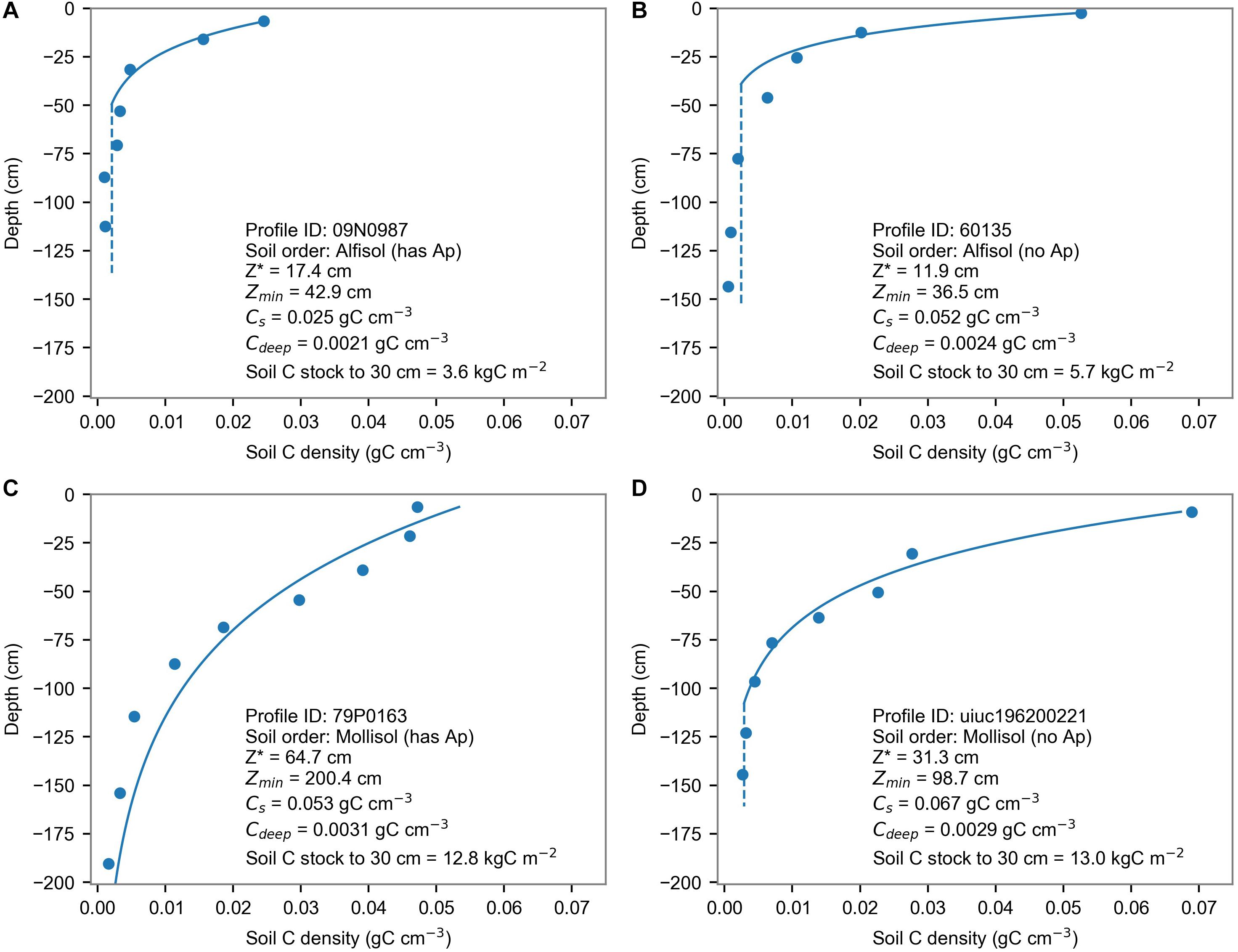
Figure 1. Four example soil depth profile fits from the ISCN database, representing two Alfisols (A,B) and two Mollisols (C,D) with an Ap horizon (A,C) and without an Ap horizon (B,D). Circles show observed carbon concentration (%), solid lines show the fit above Z_min, and dashed blue lines show the fit below Z_min.

Table 1. Profiles rejected and remaining in the analysis.

The fitting approach condensed each profile’s set of soil layers to a common set of three parameters (C_s, Z^∗, and Z_min) along with C_deep, which was calculated from the other three parameters. This facilitated a harmonized synthesis and statistical analysis of patterns of SC attenuation with depth across the large ISCN database of soil profiles. For fits using C density (which incorporated bulk density), Eq. 1 was integrated vertically to calculate total SC stock in the profile to any specified depth (assuming no changes in C_deep with depth):

For this analysis, we calculated SC stocks to 30-cm depth to examine landscape variations in topsoils. However, future analyses using this dataset could extend to deeper depths as long as shallower profiles were excluded to avoid extrapolation beyond measured profile depths.

Statistical Analyses

We focused our statistical analyses on the distribution of soil profile parameters (from the fitting procedure described above) as they varied across soil order, spatial areas, and landcover types. We used a Chi² test (R command: chisq.test) to determine differences in the distributions of the binned response variables (Z^∗, Z_min, C_surf, C_deep, C_stock). For these non-normally distributed response variables, we determined medians and 95% confidence intervals around the medians using the mean of 10,000 replicates generated using bootstrap resampling (R command: sample). Differences in mean response variables among the land cover classes by Ap horizon were tested using analysis of variance (R command: aov) and post hoc differences were determined using Tukey’s Honest Significance Difference test (R command: TukeyHSD); we tested for interactions between land cover class and Ap horizon. To test for differences between forested and unforested land cover classes, we re-grouped the samples into forested and unforested types. In addition to examining distributions pooled across the whole dataset, we controlled for spatial variations in climate and other drivers by dividing the Continental United States into a 0.5° (latitude/longitude) spatial grid. Profiles within each grid cell were further divided based on soil order, and depth distribution parameters were compared between the sets of profiles with or without an Ap horizon within each group sharing a grid cell and soil order using a paired t-test (R command: t.test, paired = T). Statistical analyses were done using R statistical software (R Core Team, 2019), and the scipy (Virtanen et al., 2020), numpy (van der Walt et al., 2011), statsmodels (Seabold and Perktold, 2010), and Matplotlib (Hunter, 2007) python packages.

Results

The ISCN database included 71,134 total profiles, but not all were suitable for the depth profile fitting approach (Table 1). 16% of profiles lacked any sampled mineral soil layers with C concentration measurements, and 56% lacked any sampled mineral soil layers with both C concentration and bulk density information necessary for determining C density. Confidently interpreting a depth profile required at least five measured layers, removing an additional 27% of profiles for %C and 14% of profiles for C density. Some of the remaining profiles were excluded because they did not yield successful fits due to non-convergence of the fitting algorithm or yielded unrealistic results (e.g., Z^∗ < 0). These steps left 38,612 C concentration profiles (54% of all profiles) and 20,151 C density profiles (28%) on which further analysis was possible. Removing profiles with R² < 0.9 further reduced the number of included C concentration profiles by 23% of successfully fitted profiles, and C density profiles by 28% of successfully fitted profiles. We repeated the analysis using an R² cutoff of 0.75, which did not substantially affect the results (see Supplementary Material). We also repeated the analysis using only profiles that reported organic C, which yielded similar results.

A large fraction of successful fits had high R² values (Figures 2A,B). Z^∗ values had an approximately log-normal distribution across the database, peaking between 10 and 30 cm for both C density and C concentration but with a long tail indicating significant numbers of soil profiles with more gradual declines in C concentration with depth (Figures 2B,C). C_s values had similar log-normal distributions centered around 1–2% C with a small number of profiles having surface C concentrations greater than 10% for C concentration, and centered around 0.01–0.03 g C cm^–3 with a small number of profiles having surface C densities greater than 0.15 g C cm^–3.

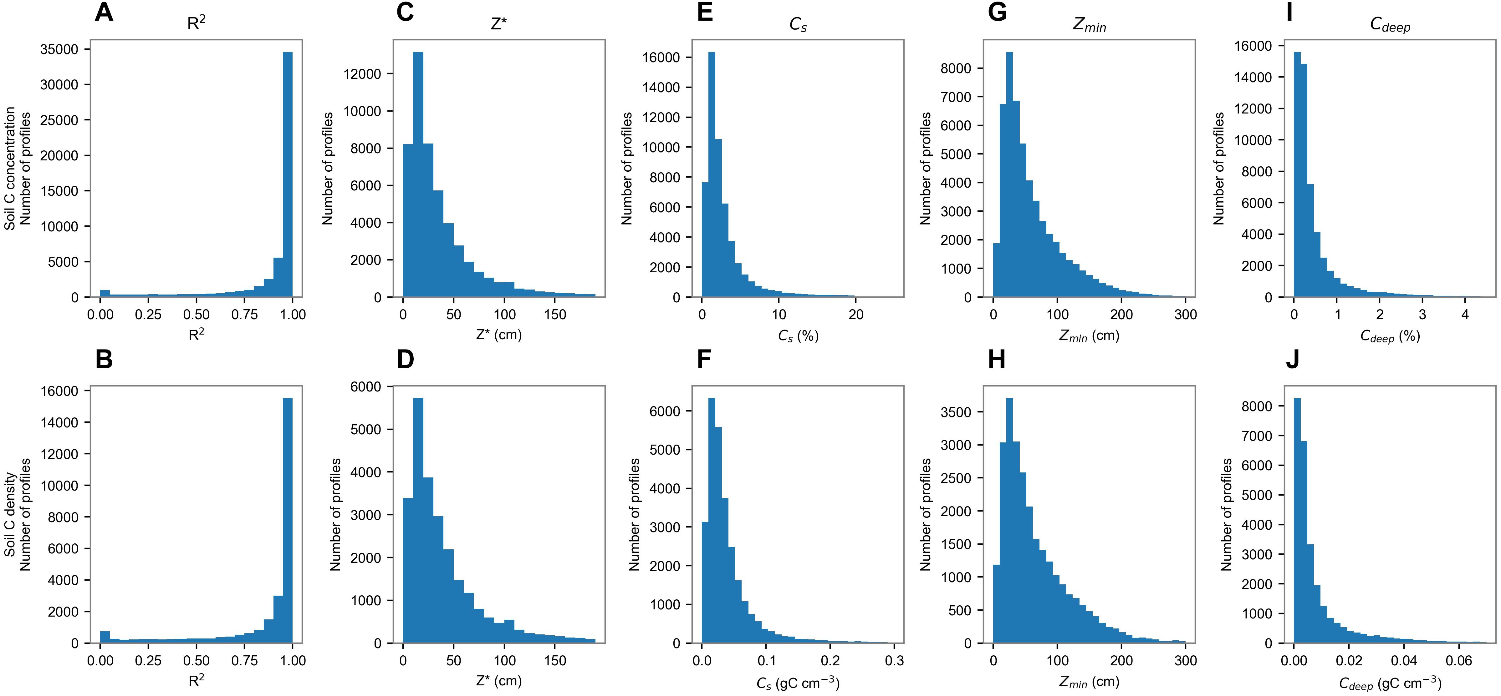
Figure 2. Distribution of key profile fit statistics for SC concentration (A,C,E,G,I) and SC density (B,D,F,H,J) profiles.

The vast majority of fitted profiles in the ISCN database were located in the Continental United States (Figure 3). This was largely due to the prevalence of soil profiles from NRCS surveys, which made up approximately 87% of the analyzed data. Thus, we focused our analysis on profiles within the Continental United States (Figure 4). C stocks calculated to 30 cm ranged up to 15 kg C m^–2, with the highest stocks occurring in the Northwest and central plains regions. The deepest SC profiles, as indicated by Z^∗ and Z_min values, were located in the central plains region. C_s and C_deep did not have clear continental-scale spatial patterns.

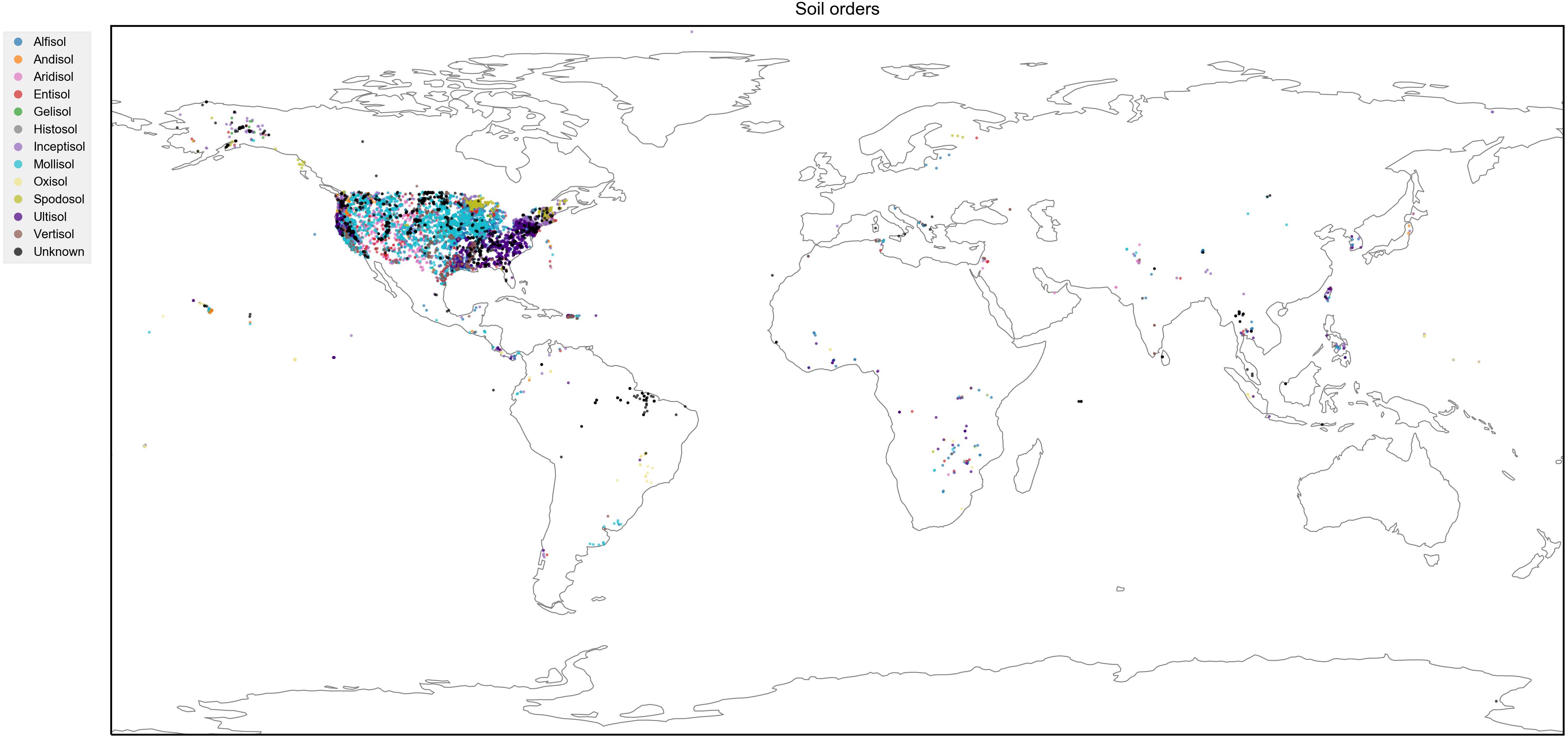
Figure 3. Spatial distribution of profiles with significant fits to Equation 1 shown according to soil order.

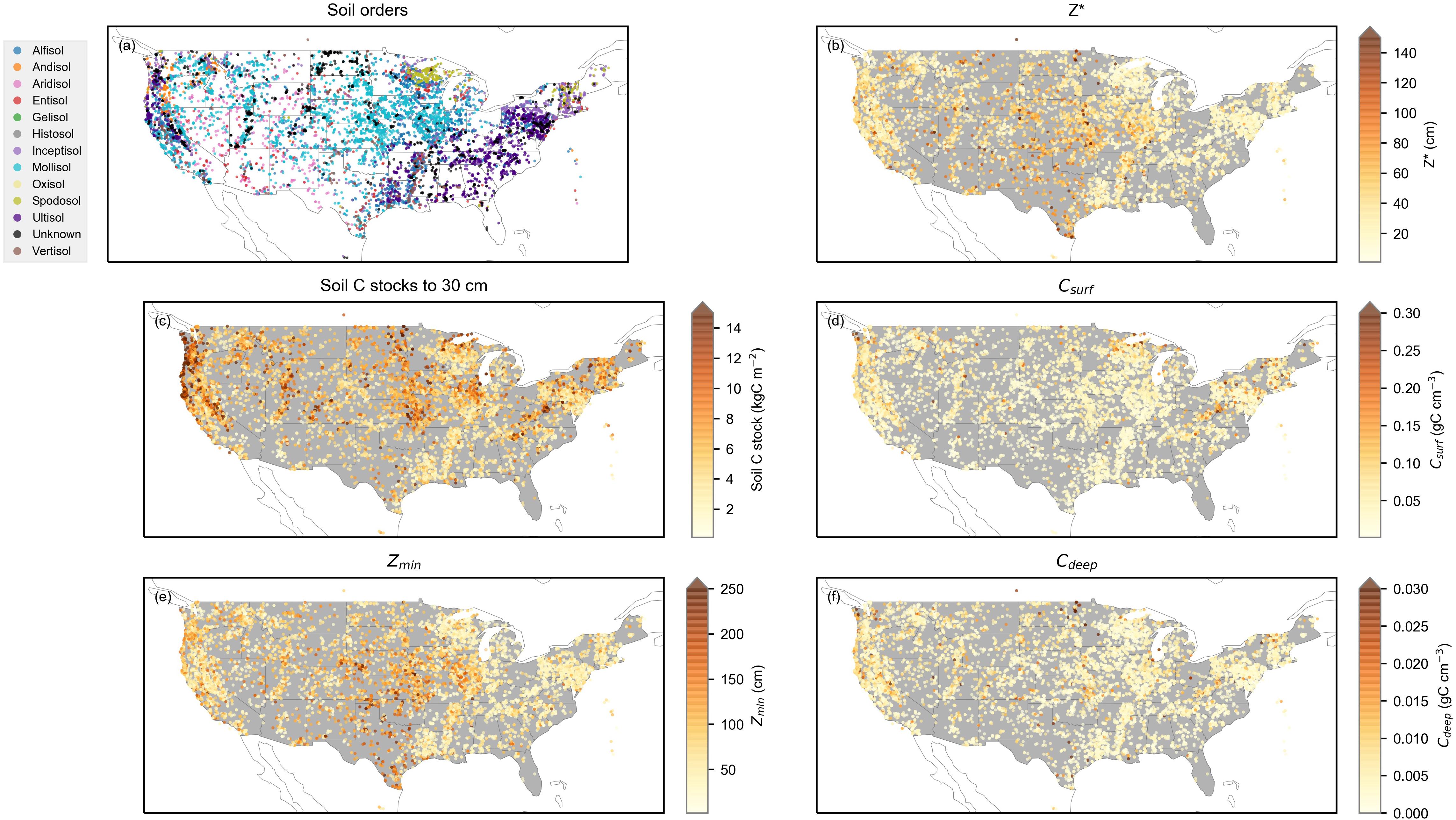
Figure 4. Spatial distributions of profile soil order and key profile parameters in the Continental United States. (a) Soil order of each profile. (b) Z^∗ value for each profile. (c) Calculated SC stock to 30 cm for each profile. (d) C_s value for each profile. (e) Z_min value for each profile. (f): C_deep value for each profile.

A key hypothesis of this analysis was that historical disturbance of the soil profile through tillage would influence SC stocks and their vertical distributions. Thus, we analyzed how soil depth distribution parameters and integrated profile C stocks varied between soil profiles with and without an Ap horizon indicating a history of tillage (Figure 5). The distribution of Z^∗ differed significantly between soils with and without an Ap horizon (Chi² = 100,899, d.f. = 187, P < 0.0001). Pooled over all soil orders, the distribution of profiles with an Ap horizon was skewed toward higher Z^∗ values (median: 26.0 ± 0.9 cm) compared to the distribution of profiles without an Ap horizon (median: 18.7 ± 0.5 cm). This indicates that SC concentrations decreased more slowly with depth in profiles with a history of tillage. Because deep-rooted plants and thick SC-rich horizons are a key characteristic of Mollisols, we separately investigated depth parameter distributions within Mollisol soil profiles. These distributions yielded similar results to all soils (Chi² = 17,074, d.f. = 187, P < 0.0001), with the distribution of Z^∗ in Mollisol profiles with Ap horizons skewed toward higher Z^∗ than non-Ap profiles (Medians: Has Ap = 42 ± 1 cm; No Ap = 31 ± 2 cm). The Z^∗ distribution for Mollisols was centered at deeper values (median: 37 ± 2 cm) than the Z^∗ distribution for all soils (median: 22 ± 1 cm; Chi² = 161380, d.f. = 187, P < 0.0001).

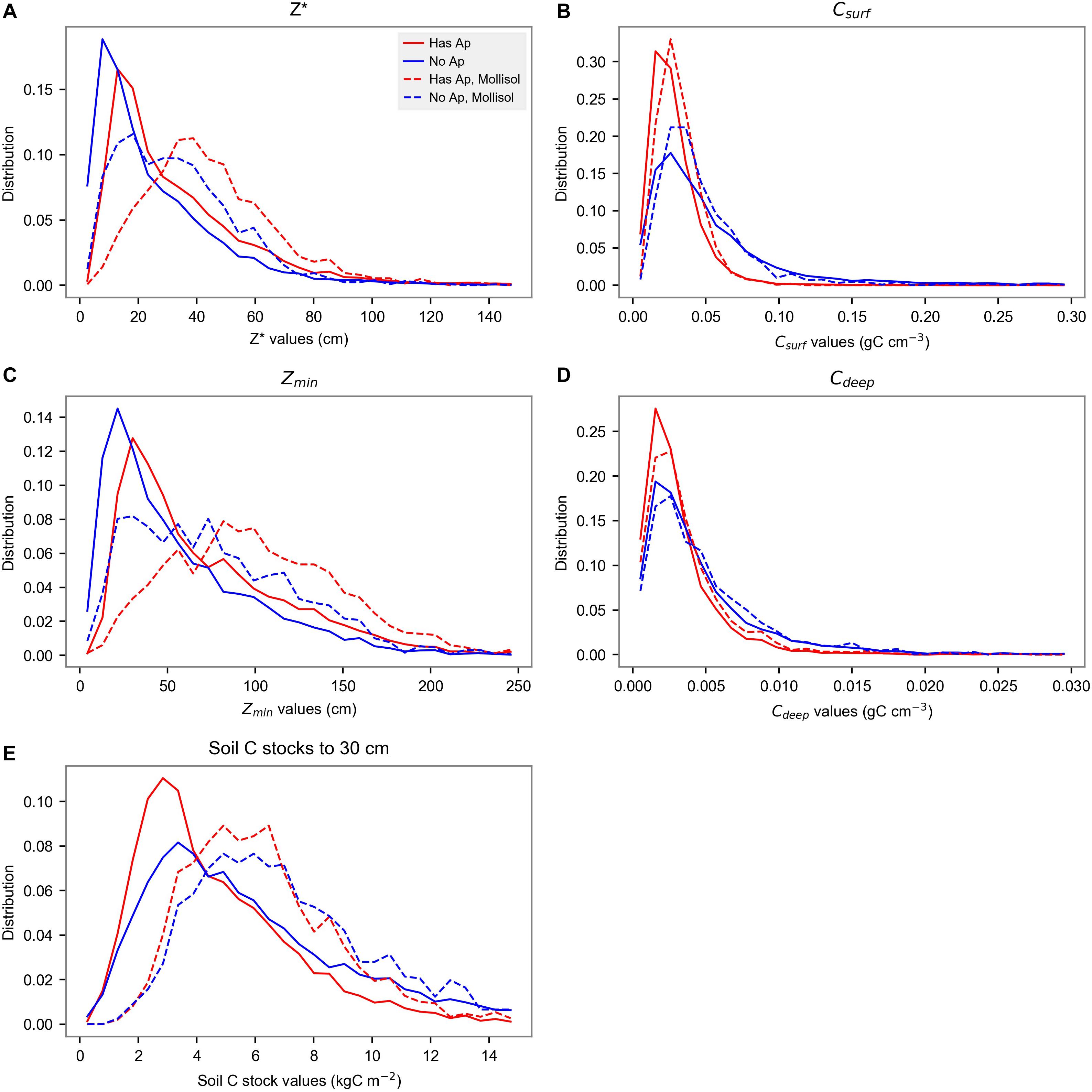
Figure 5. Distribution of soil profile parameters with Ap horizons (red) and without Ap horizons (blue). Solid lines show distributions for all soil profiles, and dashed lines show distributions for Mollisols. (A) Z^∗. (B) C_s. (C) Z_min. (D) C_deep. (E) Integrated SC stock to 30 cm.

Differences in soil profile parameter distributions with tillage history were also reflected in C_s, Z_min, C_deep, and total profile C stock. The distribution of C_s was narrower and had a higher fraction of low C_s values for profiles with Ap horizons compared to profiles without Ap horizons (Chi² = 168,000, d.f. = 199, P < 0.0001), indicating a lower incidence of high surface C concentrations, which was consistent with physical mixing of a SC-rich surface layer into deeper layers. Z_min distributions were skewed toward deeper Z_min for profiles with Ap horizons (Medians: Has Ap = 58 ± 2 cm, No Ap = 43 ± 1 cm; Chi² = 42551, d.f. = 99, P < 0.0001) and were much broader and deeper for Mollisols than for all soils (Chi² = 70,900, d.f. = 99, P < 0.0001). C_deep distributions were similar between Mollisols and all soils, and distributions with Ap horizons had lower median C density than soils without Ap horizons (Medians: Has Ap = 0.0024 ± 0.0000 g cm^–3, No Ap = 0.0033 ± 0.0000 g cm^–3), while distributions of C_deep for profiles without Ap horizons had a longer tail of higher values (Chi² = 276628, d.f. = 345, P < 0.0001). The distributions of SC stocks to 30 cm were centered around higher stocks for Mollisols than for all soils (Medians: Mollisol = 6.3 ± 0.3 kg C m^–2, All soil = 4.7 ± 0.1 kg C m^–2, Chi² = 164062, d.f. = 335, P < 0.0001), and soils with Ap horizons were somewhat skewed toward lower SC stocks and contained fewer profiles with high SC stocks (Medians: Has Ap = 4.0 ± 0.1 kg C m^–2, No Ap = 5.2 ± 0.1 kg C m^–2; Chi² = 94397, d.f. = 335, P < 0.0001).

Land cover affects SC stocks and their depth distributions and may interact with land use history (for example, previously tilled soils in some areas have been reforested). We used NLCD data to identify land cover classes for each profile and calculated mean profile parameters for profiles with or without Ap horizons within the most common land cover types (Figures 6A–C). Generally, profiles with Ap horizons had lower C_s [F₍₁,₉₀₄₄₎ = 1160, P < 0.0001] and lower SC stocks over 0 to 30 cm depth [F₍₁,₉₀₄₄₎ = 457, P < 0.0001]. Grasslands had the highest Z^∗ values and deciduous forests had the lowest. Forests had lower Z^∗ [F₍₁,₉₀₅₆₎ = 663, P < 0.0001] and higher C_s [F₍₁,₉₀₅₄₎ = 358, P < 0.0001] than non-forest landcover types. However, profiles with Ap horizons had similar mean C_s for all landcover types, with the exceptions of mixed and evergreen forests. Note that non-crop profiles with Ap horizons could represent previously tilled soils that were subsequently converted to other land cover types (e.g., reforested), but may also include agricultural sites that were not detected in the satellite-based landcover products.

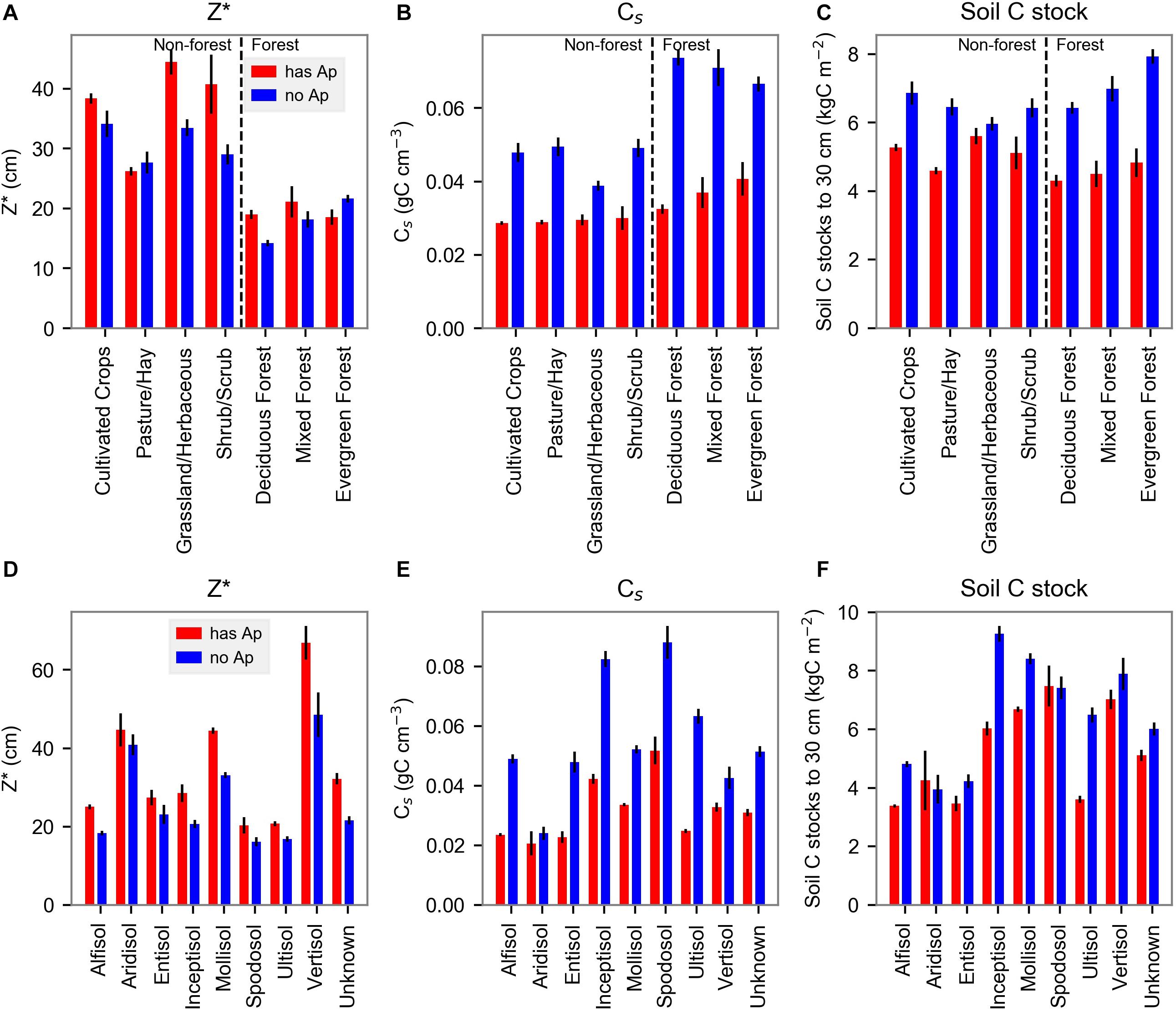
Figure 6. Mean Z*, C_s, and SC-stocks-to-30 cm for profiles with and without Ap horizons grouped according to NLCD land cover type (A–C) or profile soil order (D–F). Error bars show the standard error of the mean.

Ap horizon differences were also consistent when soils were divided by soil order (Figures 6D–F). Across all soil orders, the presence of an Ap horizon increased Z^∗ by 9–37%. This trend was statistically significant (P < 0.01) except in Aridisols, Entisols, Spodosols, and Ultisols (Figure 6D). The presence of an Ap horizon decreased C_s by 12–59%, which was statistically significant except in Aridisols and Vertisols (Figure 6E). The presence of an Ap horizon significantly decreased SC stock to 30 cm by 15–46% (P < 0.01) except in Aridisols, Entisols, Spodosols, and Vertisols, where there was no significant effect of the Ap horizon (P > 0.10, Figure 6F).

To control for climatic and regional factors, we divided the Continental United States into a 0.5° (latitude and longitude) spatial grid and calculated pooled differences in integrated SC stocks to 30 cm between profiles with or without Ap horizons within the same soil order for each grid cell (Figure 7). This grid spacing was likely too coarse to control for many differences in soil forming factors but did allow for the control of continental-scale climate and spatial biases. Note that the purpose of this stratification was not to conduct an explicit spatial or regional analysis, but only to facilitate comparisons between profiles while mitigating confounding effects due to spatial variations in climate and soil order. When combining soil orders within each grid cell, profiles with Ap horizons had significantly lower SC stocks than profiles without Ap horizons (t = −8.23, d.f. = 852, P < 0.0001). The distribution of differences between profiles from the same soil order and grid cell with and without Ap horizons was skewed toward negative values, with a long tail of cells where Ap horizons were associated with more than 5 kg C m^–2 lower SC stocks (Figure 7C). When expressed as a percentage difference in SC stock between profiles with and without Ap horizons, the skew was more apparent, with a median percent difference of 17% lower SC stocks in profiles with Ap horizons compared to profiles without Ap horizons within a grid cell and soil order (Figure 7D). A quarter of grid cells had more than 40% lower SC stocks in profiles with Ap horizons than profiles of the same soil order without Ap horizons. SC stocks in soils with Ap horizons had a significant linear relationship [Intercept: 2.77 (95% CI: 2.4, 3.2) kg C m^–2; Slope: 0.35 (95% CI: 0.30, 0.40); P < 0.0001, R² = 0.18, RMSE = 3.3 kg C m^–2] with SC stocks in soils without Ap horizons within the same grid cell and soil order (Figure 8). The slope of the relationship being below 1 indicates that profiles with Ap horizons had systematically lower SC stocks than profiles without Ap horizons and that the potential for topsoil SC loss under tillage increases with the magnitude of untilled SC stock.

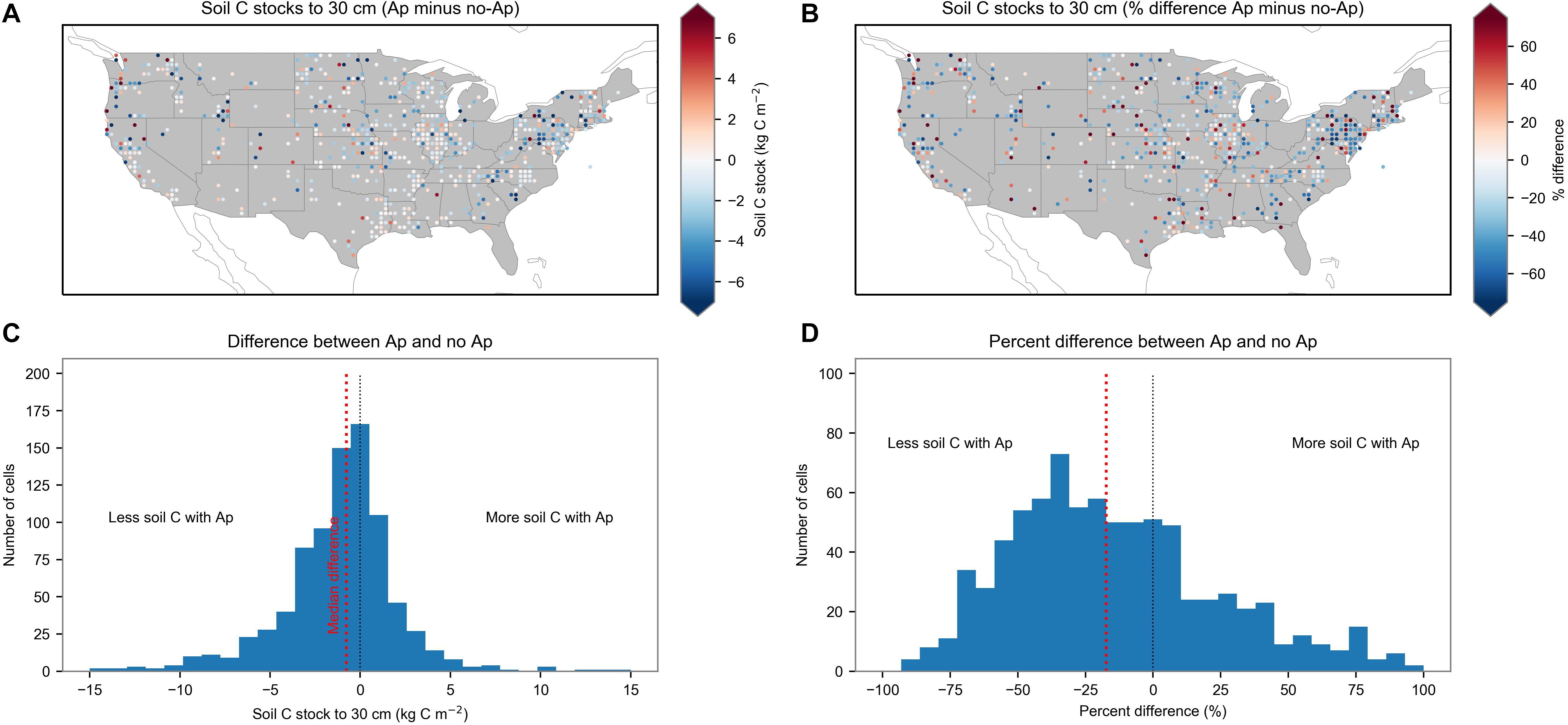
Figure 7. Differences in SC stocks to 30 cm between profiles with and without Ap horizons within each 0.5° grid cell. (A) Mean difference in each grid cell, pooled over all soil orders. (B) Mean percent difference in each grid cell, pooled over all soil orders. (C) Distribution of mean differences in SC stock for profiles within the same grid cell and soil order. The red dotted line indicates the median value of the distribution. (D) Distribution of mean percent differences in SC stock for profiles within the same grid cell and soil order. The red dotted line indicates the median value of the distribution.

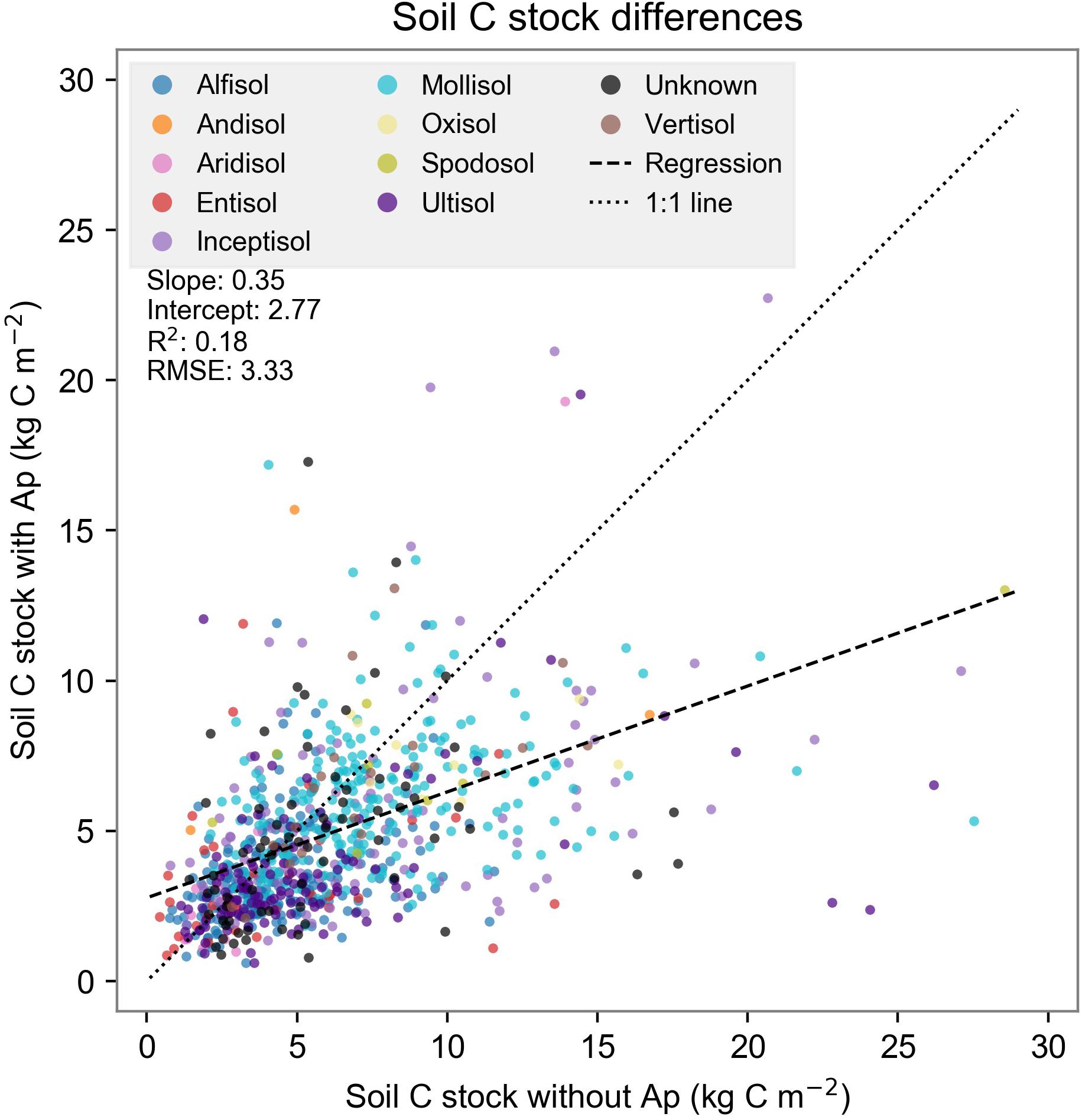
Figure 8. Mean profile SC stocks to 30 cm within each spatial grid area and soil order, compared based on presence or absence of Ap horizon. Dotted line shows a 1:1 relationship, and dashed line shows a linear regression. Points below the 1:1 line indicate that profiles with an Ap horizon had lower SC stocks than profiles without an Ap horizon within the same soil order and spatial area.

Discussion

Large datasets of soil profiles offer opportunities to examine spatial variations in biogeochemistry using a number of statistical or mathematical approaches, and we found that applying a common analysis to SC data elucidated patterns of C density and concentration with depth. The high R² values for the vast majority of soil profiles with enough depth points to fit (R² ≥ 0.9 for more than 29,000 SC concentration profiles and more than 14,000 SC density profiles; Table 1 and Figure 2) indicated that this method was successful in determining profile parameters across the dataset. This harmonized approach addressed difficulties in comparing vertical patterns across a dataset in which the depths and layers measured were variable, and facilitated analysis of total C stocks, surface C densities, and the depth scales of the profiles in an efficient statistical framework. This approach provides advantages over gridded or spatially modeled soil datasets such as the HWSD and SoilGrids. In particular, the parameters in our analysis are traceable back to individual measured profiles rather than being averaged or statistically modeled using spatial relationships or environmental covariates. This allowed depth patterns to be investigated for individual sites in the context of their profile properties and land use histories.

Depth characterization of SC by the formulation of Eq. 1 elucidates some important attributes that may be generalizable and useful in further analyses. Parameters Z_min, C_deep, C_s, and Z^∗ likely inform different aspects of C cycling. For example, Z_min likely reflects a threshold depth above which carbon retention is dominated by biotic processes such as root input, microbial processing, and stabilization of C in the biotic medium (White et al., 2012; Lawrence et al., 2015). Below Z_min, C concentration is more likely dominated by hydrology and mineralogy. In other words, Z_min represents a “biotic” vs. “quasi-biotic” transition. Such thresholds for C storage and turnover were discussed by Lawrence et al. (2015) as being closely coupled to surface area of clays and oxides, reaching a saturation level that changes with mineral transformations occurring in the B horizon subsoil. White et al. (2012) also reported that such a threshold in soil depth exists for soil mineral transformations because of the abrupt changes in hydrology, porosity, and redox reactions. Significantly, the parameter C_deep and its upper depth limit Z_min reflect a metric for detecting a fraction of C stocks that has been insulated from surface processes under historical conditions, and that may be transformed under new conditions that alter Z_min, such as an increase in rooting depth. Thus, upon shifts in ecosystem and/or management factors that change Z_min, deep carbon may be more readily decomposed (Hicks Pries et al., 2018). Meanwhile it is clear that the C_s parameter is sensitive to land cover and varies spatially. C_s was systematically higher in forests than in grasslands, crops, or shrublands, most likely due to the higher aboveground fraction of litter deposition in forests compared to the larger fraction of NPP allocated to fine roots in non-forests (Figure 6B). The Z^∗ parameter, or “e-folding” for the depth curve, was generally higher in grasslands and croplands than in forests, potentially due to deeper fine root distributions (Figure 6A). However, the variability in Z^∗ and its dependence on a range of biotic and abiotic processes provides ample opportunities for further analysis.

Land cover and land use histories were tied to significant variations in SC depth parameters. Profiles with and without an Ap horizon (indicating a history of tillage) showed legacies in agricultural disturbance that affected SC stocks and their vertical distributions. Tillage was associated with lower surface C, a more gradual decline (higher Z^∗) in C density with depth, and slightly lower C stocks integrated to 30 cm (Figures 5, 6). These effects are consistent with tillage mixing SC from the surface through the plow layer of the soil profile. Differences in historically tilled soils were evident even in profiles with non-agricultural land covers, suggesting that subsequent changes in land cover (e.g., reforestation) did not erase the impact of tillage history. These results are consistent with previous studies (Baker et al., 2007; Angers and Eriksen-Hamel, 2008; Sanderman et al., 2017; Nave et al., 2018).

Comparison of profiles within a grid of constrained spatial areas (Figure 7A) was consistent with the overall finding that tillage history was associated with lower C stocks for topsoils (to a depth of 30 cm). While previous studies have relied on spatial modeling (e.g., Sanderman et al., 2017) or extrapolated results from a limited number of observations (e.g., Angers and Eriksen-Hamel, 2008), our analysis recovers these tillage-SC relationships from a large, broadly distributed dataset of tens of thousands of soil profile measurements traceable back to individual profiles.

In addition to the current analysis, the database of soil depth distribution parameters produced by our analysis has broad potential applications for constraining depth patterns of SC in both empirical and modeling analyses. Current land surface models are now incorporating depth distributions of SC stocks by modeling SC dynamics across multiple layers (e.g., Koven et al., 2013; Burke et al., 2017), though such models have not yet generally included agricultural tillage effects on SC cycling. Our database provides a potential tool for evaluating different model formulations and parameterizations based on the simulated depth distributions of SC stocks in addition to databases of total C stocks (to specified depth) that are commonly used in model evaluation. The use of individual profiles rather than a spatially averaged, gridded database allows variations in SC profiles due to variations in land use history, ecosystem type, and topography to be compared. This could allow land surface models that include sub-grid heterogeneity such as agricultural versus forest lands (e.g., Shevliakova et al., 2009) to be evaluated by comparing sub-grid fractions directly with appropriately matched measurements rather than averaging over sub-grid variability. Our database can also facilitate large-scale analysis of controls on SC depth distributions such as topography, slope and aspect, climate, and ecosystem type in addition to the land cover and land use history factors that were the focus of this analysis. While our analysis was primarily limited to the continental United States, an expanded dataset of SC depth distribution parameters could be generated from broader datasets with global distributions, such as the WoSIS database (Batjes et al., 2020).

Conclusion

We fit a harmonized depth distribution function of SC to a database of over 40,000 soil profiles across the continental United States, yielding a new database of depth distribution parameters. We used the database to compare depth parameters across soil orders, land cover classes, and land use histories. Several depth parameters were sensitive to soil order and land cover; in most cases, tillage indicated by the presence of Ap horizons reduced surface SC concentrations, increased the length scale (Z^∗) of SC decline with depth, and decreased SC stocks in the top 30 cm. The database of depth profile parameters is applicable to statistical analyses and land surface model evaluation across different ecosystem types and large spatial gradients.

Data Availability Statement

All fitting and analysis code, along with calculated depth distribution parameters for each profile, are archived at doi: 10.5281/zenodo.3924496. ISCN data are available through the ISCN data portal: http://iscn.fluxdata.org/data/access-data/database-reports/.

Author Contributions

BS analyzed the data and led writing of the manuscript. CT conducted statistical analysis. JH, LN, CK, JO’D, and BS conceived the study. YH, CT, and BS calculated depth distribution fits. UM contributed to land cover data. All authors contributed to writing and editing of the manuscript.

Funding

BS acknowledges support from the United States Department of Energy, Office of Science, Office of Biological and Environmental Research, Next Generation Ecosystem Experiments (NGEE) Arctic project. ORNL is managed by UT-Battelle, LLC, for the DOE under contract DE-AC05-00OR22725. CK acknowledges support from the DOE Office of Science, Office of Biological and Environmental Research, Regional and Global Model Analysis Program through the RUBISCO SFA and Early Career Research Programs, under contract number DE-AC02-05CH11231.

Conflict of Interest

The authors declare that the research was conducted in the absence of any commercial or financial relationships that could be construed as a potential conflict of interest.

Acknowledgments

This work was facilitated by the ISCN and benefited from extensive data contributions by the USDA-Natural Resources Conservation Service (National Cooperative Soil Survey) and the United States Geological Survey.

Supplementary Material

The Supplementary Material for this article can be found online at: https://www.frontiersin.org/articles/10.3389/fenvs.2020.00146/full#supplementary-material

References

Angers, D. A., and Eriksen-Hamel, N. S. (2008). Full-Inversion tillage and organic carbon distribution in soil profiles: a meta-analysis. Soil Sci. Soc. Am. J. 72, 1370. doi: 10.2136/sssaj2007.0342
Baker, J. M., Ochsner, T. E., Venterea, R. T., and Griffis, T. J. (2007). Tillage and soil carbon sequestration—What do we really know? Agric. Ecosyst. Environ. 118, 1–5. doi: 10.1016/J.AGEE.2006.05.014
Batjes, N. H. (1996). Total carbon and nitrogen in the soils of the world. Eur. J. Soil Sci. 47, 151–163. doi: 10.1111/j.1365-2389.1996.tb01386.x
Batjes, N. H., Ribeiro, E., and van Oostrum, A. (2020). Standardised soil profile data to support global mapping and modelling (WoSIS snapshot 2019). Earth Syst. Sci. Data 12, 299–320. doi: 10.5194/essd-12-299-2020
Bruun, T. B., Elberling, B., Neergaard, A., and Magid, J. (2015). Organic carbon dynamics in different soil types after conversion of forest to agriculture. L. Degrad. Dev. 26, 272–283. doi: 10.1002/ldr.2205
Burke, E. J., Chadburn, S. E., and Ekici, A. (2017). A vertical representation of soil carbon in the JULES land surface scheme (vn4.3_permafrost) with a focus on permafrost regions. Geosci. Model Dev. 10, 959–975. doi: 10.5194/gmd-10-959-2017
Ciais, P., Sabine, C., Bala, G., Bopp, L., Brovkin, V., Canadell, J., et al. (2013). “Carbon and Other Biogeochemical Cycles,” in Climate Change 2013 - The Physical Science Basis, ed. Intergovernmental Panel on Climate Change (Cambridge: Cambridge University Press), 465–570. doi: 10.1017/CBO9781107415324.015
Davidson, E. A., Savage, K. E., Trumbore, S. E., and Borken, W. (2006). Vertical partitioning of CO2 production within a temperate forest soil. Glob. Chang. Biol. 12, 944–956. doi: 10.1111/j.1365-2486.2005.01142.x
Doetterl, S., Berhe, A. A., Nadeu, E., Wang, Z., Sommer, M., and Fiener, P. (2016). Erosion, deposition and soil carbon: a review of process-level controls, experimental tools and models to address C cycling in dynamic landscapes. Earth Sci. Rev. 154, 102–122. doi: 10.1016/j.earscirev.2015.12.005
Eglin, T., Ciais, P., Piao, S. L., Barre, P., Bellassen, V., Cadule, P., et al. (2010). Historical and future perspectives of global soil carbon response to climate and land-use changes. Tellus Ser. B Chem. Phys. Meteorol. 62, 700–718. doi: 10.1111/j.1600-0889.2010.00499.x
Fry, J. A., Xian, G., Jin, S. M., Dewitz, J. A., Homer, C. G., Yang, L. M., et al. (2011). Completion of the 2006 national land cover database for the conterminous United States. Photogramm. Eng. Remote Sens. 77, 858–864.
Harden, J. W., Sharpe, J. M., Parton, W. J., Ojima, D. S., Fries, T. L., Huntington, T. G., et al. (1999). Dynamic replacement and loss of soil carbon on eroding cropland. Global Biogeochem. Cycles 13, 885–901. doi: 10.1029/1999GB900061
Hengl, T., De Jesus, J. M., MacMillan, R. A., Batjes, N. H., Heuvelink, G. B. M., Ribeiro, E., et al. (2014). SoilGrids1km - Global soil information based on automated mapping. PLoS One 9:e0105992. doi: 10.1371/journal.pone.0105992
Hicks Pries, C. E., Sulman, B. N., West, C., O’Neill, C., Poppleton, E., Porras, R. C., et al. (2018). Root litter decomposition slows with soil depth. Soil Biol. Biochem. 125, 103–114. doi: 10.1016/j.soilbio.2018.07.002
Homer, C., Dewitz, J., Yang, L., Jin, S., Danielson, P., Xian, G., et al. (2015). Completion of the 2011 national land cover database for the conterminous United States–representing a decade of land cover change information. Photogramm. Eng. Remote Sens. 81, 345–354.
Homer, C., Huang, C., Yang, L., Wylie, B., and Coan, M. (2004). Development of a 2001 national land-cover database for the United States. Photogramm. Eng. Remote Sens. 70, 829–840. doi: 10.14358/PERS.70.7.829
Houghton, R. A., House, J. I., Pongratz, J., Van Der Werf, G. R., Defries, R. S., Hansen, M. C., et al. (2012). Carbon emissions from land use and land-cover change. Biogeosciences 9, 5125–5142. doi: 10.1016/j.scitotenv.2018.07.317
Hunter, J. D. (2007). Matplotlib: a 2D graphics environment. Comput. Sci. Eng. 9, 90–95. doi: 10.1109/MCSE.2007.55
Jobbágy, E. G., and Jackson, R. B. (2000). The vertical distribution of soil organic carbon and its relation to climate and vegetation. Ecol. Appl. 10, 423–436. doi: 10.1890/1051-0761(2000)010[0423:tvdoso]2.0.co;2
Koven, C. D., Riley, W. J., Subin, Z. M., Tang, J. Y., Torn, M. S., Collins, W. D., et al. (2013). The effect of vertically resolved soil biogeochemistry and alternate soil C and N models on C dynamics of CLM4. Biogeosciences 10, 7109–7131. doi: 10.5194/bg-10-7109-2013
Lal, R., and Kimble, J. M. (2000). “Pedogenic carbonates and the global carbon cycle,” in Global Climate Change and Pedogenic Carbonates, eds R. Lal, J. M. Kimble, H. Eswaran, and B. A. Stewart (Boca Raton, FL: CRC Press), 1–14.
Lawrence, C. R., Harden, J. W., Xu, X., Schulz, M. S., and Trumbore, S. E. (2015). Long-term controls on soil organic carbon with depth and time: a case study from the Cowlitz River Chronosequence, WA USA. Geoderma 247–248, 73–87. doi: 10.1016/j.geoderma.2015.02.005
Mann, L. K. (1985). A regional comparison of carbon in cultivated and uncultivated alfisols and mollisols in the central United States. Geoderma 36, 241–253. doi: 10.1016/0016-7061(85)90005-9
Meersmans, J., Van Wesemael, B., De Ridder, F., Dotti, M. F., De Baets, S., and Van Molle, M. (2009). Changes in organic carbon distribution with depth in agricultural soils in northern Belgium, 1960-2006. Glob. Chang. Biol. 15, 2739–2750. doi: 10.1111/j.1365-2486.2009.01855.x
Nachtergaele, F., van Velthuizen, H., Verelst, L., Batjes, N. H., Dijkshoorn, K., van Engelen, V. W. P., et al. (2010). “The harmonized world soil database,” in in Proceedings of the 19th World Congress of Soil Science, Soil Solutions for a Changing World, Brisbane, 34–37.
Nave, L. E., Domke, G. M., Hofmeister, K. L., Mishra, U., Perry, C. H., Walters, B. F., et al. (2018). Reforestation can sequester two petagrams of carbon in US topsoils in a century. Proc. Natl. Acad. Sci. U.S.A. 115:201719685. doi: 10.1073/pnas.1719685115
Nave, L. E., Johnson, K., van Ingen, C., Agarwal, D., Humphry, M., and Beekwilder, N. (2016). International Soil Carbon Network (ISCN) Database v3. Oak Ridge, TN: U.S. Department of Energy Office of Scientific and Technical Information, doi: 10.17040/ISCN/1305039
Nave, L. E., Swanston, C. W., Mishra, U., and Nadelhoffer, K. J. (2013). Afforestation effects on soil carbon storage in the United States: a synthesis. Soil Sci. Soc. Am. J. 77, 1035. doi: 10.2136/sssaj2012.0236
Nave, L. E., Walters, B. F., Hofmeister, K. L., Perry, C. H., Mishra, U., Domke, G. M., et al. (2019). The role of reforestation in carbon sequestration. New For. 50, 115–137. doi: 10.1007/s11056-018-9655-3
Rosenbloom, N. A., Harden, J. W., Neff, J. C., and Schimel, D. S. (2006). Geomorphic control of landscape carbon accumulation. J. Geophys. Res. 111:G01004. doi: 10.1029/2005JG000077
Rumpel, C., and Kögel-Knabner, I. (2011). Deep soil organic matter—a key but poorly understood component of terrestrial C cycle. Plant Soil 338, 143–158. doi: 10.1007/s11104-010-0391-5
Sanderman, J., Hengl, T., and Fiske, G. J. (2017). Soil carbon debt of 12,000 years of human land use. Proc. Natl. Acad. Sci. U.S.A. 114, 9575–9580. doi: 10.1073/pnas.1706103114
Schmidt, M. W. I., Torn, M. S., Abiven, S., Dittmar, T., Guggenberger, G., Janssens, I. A., et al. (2011). Persistence of soil organic matter as an ecosystem property. Nature 478, 49–56. doi: 10.1038/nature10386
Seabold, S., and Perktold, J. (2010). “Statsmodels: econometric and statistical modeling with python,” in Proceedings of the 9th Python in Science Conference, Montreal: Cirano.
Senthilkumar, S., Basso, B., Kravchenko, A. N., and Robertson, G. P. (2009). Contemporary evidence of soil carbon loss in the U.S. corn belt. Soil Sci. Soc. Am. J. 73, 2078–2086. doi: 10.2136/sssaj2009.0044
Shevliakova, E., Pacala, S. W., Malyshev, S., Hurtt, G. C., Milly, P. C. D., Caspersen, J. P., et al. (2009). Carbon cycling under 300 years of land use change: importance of the secondary vegetation sink. Global Biogeochem. Cycles 23:GB2022. doi: 10.1029/2007GB003176
Six, J., Elliott, E., and Paustian, K. (2000). Soil macroaggregate turnover and microaggregate formation: a mechanism for C sequestration under no-tillage agriculture. Soil Biol. Biochem 32, 2099–2103. doi: 10.1016/S0038-0717(00)00179-6
Soil Survey Staff (2014). Keys to Soil Taxonomy, 12th ed. Washington, DC: USDA-Natural Resources Conservation Service.
Sun, T., Wang, Y., Hui, D., Jing, X., and Feng, W. (2020). Soil properties rather than climate and ecosystem type control the vertical variations of soil organic carbon, microbial carbon, and microbial quotient. Soil Biol. Biochem. 107905. (in press). doi: 10.1016/j.soilbio.2020.107905
van der Walt, S., Colbert, S. C., and Varoquaux, G. (2011). The NumPy array: a structure for efficient numerical computation. Comput. Sci. Eng. 13, 22–30. doi: 10.1109/MCSE.2011.37
Virtanen, P., Gommers, R., Oliphant, T. E., Haberland, M., Reddy, T., Cournapeau, D., et al. (2020). SciPy 1.0: fundamental algorithms for scientific computing in Python. Nat. Methods 17, 261–272. doi: 10.1038/s41592-019-0686-2
Vogelmann, J. E., Howard, S. M., Yang, L., Larson, C. R., Wylie, B. K., and Van Driel, N. (2001). Completion of the 1990s national land cover data set for the conterminous united states from landsat thematic mapper data and ancillary data sources. Photogramm. Eng. Remote Sensing 67, 650–655.
White, A. F., Schulz, M. S., Vivit, D. V., Bullen, T. D., and Fitzpatrick, J. (2012). The impact of biotic/abiotic interfaces in mineral nutrient cycling: a study of soils of the Santa Cruz chronosequence. California. Geochim. Cosmochim. Acta 77, 62–85. doi: 10.1016/j.gca.2011.10.029
Keywords: soil, soil carbon, depth, tillage, land use
Citation: Sulman BN, Harden J, He Y, Treat C, Koven C, Mishra U, O’Donnell JA and Nave LE (2020) Land Use and Land Cover Affect the Depth Distribution of Soil Carbon: Insights From a Large Database of Soil Profiles. Front. Environ. Sci. 8:146. doi: 10.3389/fenvs.2020.00146
Received: 16 December 2019; Accepted: 29 July 2020;
Published: 25 August 2020.
Edited by:
Marion Schrumpf, Max Planck Institute for Biogeochemistry, GermanyReviewed by:
Zamir Libohova, United States Department of Agriculture (USDA), United StatesGerrit Angst, Institute of Soil Biology (ASCR), Czechia
Copyright © 2020 Sulman, Harden, He, Treat, Koven, Mishra, O’Donnell and Nave. This is an open-access article distributed under the terms of the Creative Commons Attribution License (CC BY). The use, distribution or reproduction in other forums is permitted, provided the original author(s) and the copyright owner(s) are credited and that the original publication in this journal is cited, in accordance with accepted academic practice. No use, distribution or reproduction is permitted which does not comply with these terms.
*Correspondence: Benjamin N. Sulman, sulmanbn@ornl.gov