An Idealized Landslide Failure Surface and Its Impacts on the Traveling Paths

1. Introduction

Landslides, slope failures and the sequential mass movements caused by heavy or abnormal rainfalls often take place in mountainous areas and sometimes cause huge damages to property and people (Dong et al., 2011; Lin et al., 2011; Iverson et al., 2015; Zhang et al., 2018). The volume of the released mass and its impact area generally determine the scale of the disaster. However, the estimation of the released volume and the prediction of the sequential flow paths of the moving mass for a landslide-prone area are still challenging tasks because of their high degree of uncertainty. Numerical simulations, founded on physics-based mechanical models (Kuo et al., 2009, 2011, 2013; Mergili et al., 2020), discrete numerical approaches (Wu, 2010; Lo et al., 2011; Song et al., 2017; Yu et al., 2019) or statistics-based empirical models (Scheidegger, 1973; Manzella and Labiouse, 2013; Chen et al., 2014; Zhan et al., 2017), are common tools for risk assessment or for evaluating mitigation or remediation measures.

In terms of scenario investigation, the identification of the area prone to landslide and the estimation of the associated volume of moving mass are crucial for performing any numerical simulation. Owing to the rapid development of modern remote sensing techniques (LiDAR, SAR, InSAR, UAVSAR, etc.), even the tiniest topographic features (micro-topography) or structure patterns can be recognized, making it possible to identify the areas susceptible to landslides or to investigate the landslide dynamics (Lin et al., 2013, 2014; Stumpf et al., 2013; Delbridge et al., 2016). For example, Lin et al. (2014) suggested a methodological approach intended for detecting the large-scale landslides of potential in southern Taiwan by using LiDAR data. That is, with the hill-shade imagines given in different azimuth based on a high-resolution LiDAR-derived Digital Elevation Map (DEM) and with the help of aerial photos and geological field investigation, one may be able to identify the outline/boundaries of an unstable area that is prone to movement, i.e., identifying the scarps of potential landslides. Applying the technique of Uninhabited Aerial Vehicle Synthetic Aperture Radar (UAVSAR), Delbridge et al. (2016) developed a method for characterizing the 3-D surface deformation. Hence, in addition to the initiation mechanism, the estimation of the failure surface for a landslide-prone area has become an issue of high priority. Nevertheless, the geometry of the failure surface is tightly linked with the local geological structure and hydrological conditions. The complex composition of the material and the infiltration pattern of groundwater add to the complexity of the problem.

In general, the failure surface can be of different shapes, but the vertical section view along the flow direction can be roughly approximated by an arc of a circle as the most common case (Briaud, 2013). Hence, in additional to 2-D cases, a spherical-shaped failure surface is often used when investigating the performance of methods for 3-D slope stability analysis (see Lam and Fredlund, 1993; Huang and Tsai, 2000; Huang et al., 2002). As the high-resolution DEMs have become popular, a geometric interpretation of the failure surface based on a DEM, the Sloping Local Base Level (SLBL) method, was proposed for studying the failure mechanism as well as for a preliminary analysis prior to field investigation (Jaboyedoff et al., 2004, 2009). The SLBL-defined sliding surface possesses a constant second derivative, so that the surface exhibits a parabolic curve along the down-slope direction. Taken into account the curvature in the transverse direction, Reid et al. (2000, 2001) suggested a spherical failure surface together with extension of Bishop's (Bishop, 1955) limit-equilibrium analysis for quantitatively assessing the three-dimensional gravitational slope stability, explicitly for the stratovolcano edifice failure with large volumes without considering the internal/local structures. This searching scheme has been extended in the software Scoops3D for slope stability assessment in the framework of a digital landscape, where the local material properties in the subsurface and the hydrological conditions (groundwater configuration) can be taken into account (Reid et al., 2015; Alvioli et al., 2018; Zhang and Wang, 2019).

The sliding surface defined by means of Scoops3D is spherical, so that there exists only one curvature. One may benefit from its simplicity for constructing the surface in the three-dimensional configuration. However, this single curvature approach is sometimes not sufficient for describing a plausible failure surface with respect to a complex topography. Recently, Kuo et al. (2020) proposed a smooth surface enclosing a given volume and with minimal surface area (volume-constrained smooth minimal surface) for mimicking the fracture interface of a deep-seated landslide, of which the boundary on the topographic surface fits that identified by the specific micro-topography through the high-resolution DEM and from a geological field survey. In Kuo et al. (2020), the smooth minimal surface is constructed under the assumption that the slope material is homogeneous and isotropic, i.e., the stratigraphy and geological structures are omitted. Nevertheless, the verification against 24 landslides triggered by excessive rainfall during the 2009 Typhoon Morakot confirms its applicability of providing acceptable predictions. Instead of the minimization of a smooth surface area, an idealized surface with two distinct curvatures in the down-slope and cross-slope directions, respectively, is suggested for mimicking the sliding surface in the present study. This concept has been motivated by the investigation on the source scars of historical events, and it provides the freedom of matching the identified surface boundary of a landslide-prone area. However, it also requests additional constraints to define a unique failure surface in this regard.

In terms of the released mass volume, this method was used to assess the failure surface of 45 landslide events (source scars) that occurred in 2009 in southern Taiwan during Typhoon Morakot (Lin et al., 2013; Tai and Jan, 2019). The results indicate that there are two specific relations for the size (length and width) of the source scar area and the failure depth, in the down-slope and cross-slope directions, respectively. These specific relations may significantly simplify the complicated process of determining surface curvature. Together with the empirical formula expressing the relation between landslide area and volume, e.g., the regressed formula in the present study or an appropriate one, such as the volume-area relation proposed by Guzzetti et al. (2009), one is able to mimic the plausible failure surface, when the area susceptible to landsliding is given. We have applied the hereby proposed idealized curved surface (ICS) to the back-calculation of the 2009 Hsiaolin Landslide event for investigating its feasibility, where a two-phase model and the associated numerical code used in Tai et al. (2019) are employed. We have then compared our results to the ones computed with the failure surface (FS) identified by post-event investigations. Not only the geometry of the surface is compared, but also the flow paths (flow-covered area) and the differences in flow thickness are examined at different time intervals, from movement initiation to deposition.

In section 2, we present the construction of the idealized curved surface, which consists of the formulation of the ICS (section 2.1), the regressed geometrical characteristics (section 2.2), and the procedure of determining the unique ICS (section 2.3). The training data of the 45 landslides are collected and listed in Appendix A, while their locations in Taiwan are depicted in Appendix B. The application of the method to the 2009 Hsiaolin Landslide is given in section 3, where the differences of the results computed with the ICS and FS are detailed. The data of the discrepancy evolutions are given in Appendix C. At last, the great application potential of the proposed ICS approach for stability assessment in variant scenarios is highlighted in the concluding remarks.

2. Idealized Surface for Failure Surface

2.1. Idealized Curved Surface

In Geographic Information System (GIS), the terrain data are generally provided in a Cartesian coordinate system. In the present study, we set the xy-plane on the horizontal plane and the z-axis accounting for the elevation. Consider a specific surface, of which the curvature in the principal direction (x-axis) reads κ_x and the curvature in the lateral direction (y-axis) is κ_y. According to the differential geometry (Bronstein et al., 1996), the surface elevation z and these curvatures are related by

where $C_x={\left\{1+{(\partial z/\partial x)}^2\right\}}^{-1/2}$ and $C_y={\left\{1+{(\partial z/\partial y)}^2\right\}}^{-1/2}$, respectively.

As shown in Figure 1A, line $\overline{p_1{p}_2}$ stands for the main (down-slope) axis of the failure area on the slope with p₁ and p₂ the upper and lower points, respectively. Line $\overline{p_3{p}_4}$ is perpendicular to the vertical section of $\overline{p_1{p}_2}$ and vertically above the midpoint of $\overline{p_1{p}_2}$. The idealized curve $\stackrel{⌢}{p_1{p}_2}$ below $\overline{p_1{p}_2}$ is indicated by the thick line in Figure 1B, in which L is the length of $\overline{p_1{p}_2}$, angle θ represents the inclination angle of $\overline{p_1{p}_2}$ to the horizon. In Figure 1B, p_m denotes the midpoint of $\overline{p_1{p}_2}$ and d_m accounts for the vertical distance (depth) from the midpoint of the idealized curve to $\overline{p_1{p}_2}$. With the geometric relation, one can easily arrive at

with R the curvature radius and θ_arc the half expanding angle. Hence, it is clear that the central curve of the idealized surface $\stackrel{⌢}{p_1{p}_2}$ along the main axis is a function of the five parameters (R, L, θ, θ_arc, d_m) or (R, L, θ, ϕ, d_m), where ϕ = θ+θ_arc is the slope angle of the surface along the main axis. In general, (L, θ) is available once the failure area is identified and the down-slope direction is defined, but the angle θ_arc is a non-linear function of d_m and R. The curvature radius R and angle θ_arc can be determined by means of iteration, once (L, θ, d_m) are given.

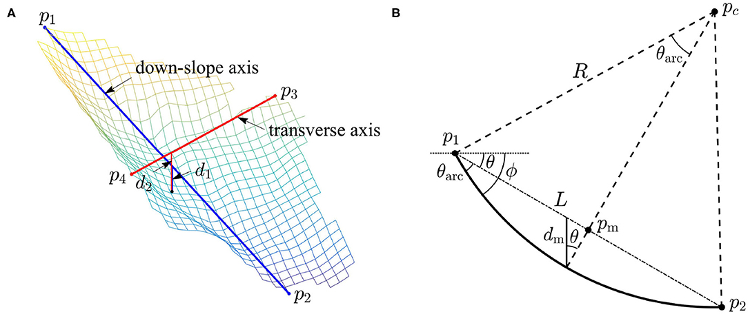
Figure 1. (A) The main (down-slope) axis, the transverse axis and the associated depths, d₁ and d₂. (B) The geometric relation between R, L, θ, and d_m.

2.2. Geometric Characteristic of the Idealized Surface

The proposed ICS is applied to mimic the failure surface of historical events. Comparing the difference between the DEMs, before and after the events, it is possible to identify the landslide area and the associated volume of the landslide mass. With the 2005 and 2010 LiDAR-derived DEMs (1 m resolution), a total of 45 landslides (source scars) that took place during Typhoon Morakot in 2009, in different catchments in Southern Taiwan, are taken into account. They are found in the catchments DF081 and DF054, in the mountainous areas of the Kao-Ping River basin and the ones by the Hsiaolin event (Lin et al., 2013; Tai and Jan, 2019). Among them, more than 470 victims have been identified in the Hsiaolin Landslide event. Being impressed by its large scale, the huge volume of released mass and the breach of the short-lived landslide dam, it has attracted particular attention of the government and engineering/scientific interests from research communities for natural hazard mitigation (Dong et al., 2011; Kuo et al., 2011, 2013; Lo et al., 2011; Tsou et al., 2011; Lin et al., 2014), and the Hsiaolin case will serve as the application example in section 3 in the present study. Because these landslides were triggered during the typhoon, for each source scar only the area with failure depth more than 0.5 m are taken into account in investigating the geometric characteristics of the ICSs for the sake of isolating the erosion at the scar boundaries during the heavy rainfall. In the classification of landslide types, proposed by Hungr et al. (2014), they are mainly debris avalanches (and potentially debris flows in some highly channelized cases). For an overview, the 45 source scars are depicted in Supplementary Figures B1–B3, in which the red boxes in the inset panel indicate their corresponding locations in Taiwan. For each scar area, 10 points at the top and 10 points on the lowest margin are selected, yielding 100 combinations. That is, we have produced 100 idealized surfaces for each source scar, of which the five parameters (R, L, θ, θ_arc, d_m) are computed, where d_m is determined with respect to the post-event surface and the system (2) is solvable. In terms of the volume of computed landslide mass, the top 10 combinations are figured out, in which the mean values of the geometric parameters, such as the curvature radius R, depth d, and length L, are taken into account. Together with the failure area A_L and the associated released volume V_L, these mean values are summarized and listed in Supplementary Tables A1, A2 for reference. It is worth noting that, in both the main down-slope and transverse directions, there are specific relations among the mean curvature radius R, depth d, and length L of the 10 best-fitted curved surfaces. They can be obtained by regression and given by

in the main down-slope direction, and

in the transverse direction, as given by the solid lines in Figures 2A,B. The mean values of the parameters and the regressed specific relations are illustrated in Figures 2A,B, where panel (A) shows the data in the down-slope direction, and panel (B) is for the data in the cross-slope direction. In Figures 2A,B,D, the solid red circles and green squares, respectively, stand for the landslides taking place in the catchments of DF081 and DF054, the magenta triangle markers represent the source scars for the Hsiaolin event, and the blue diamond markers denote the ones in the mountainous areas of the Kao-Ping River basin. Although the two regressed lines are close to each other in the plot, it is inappropriate to merge them. With the help of Figure 1B, one can find that formula (3) is close to the ideal curve with inclination angle θ = 32°, and relation (4) approximately follows the curve with θ = 10° (cf. Figure 2C). Hence, relation (3) indicates a representative inclination angle (around 32°) of $\overline{p_1{p}_2}$ in the down-slope direction, and relation (4) reflects the fact that the transverse slope (cross-slope) of the source scar is slightly tilted in general.

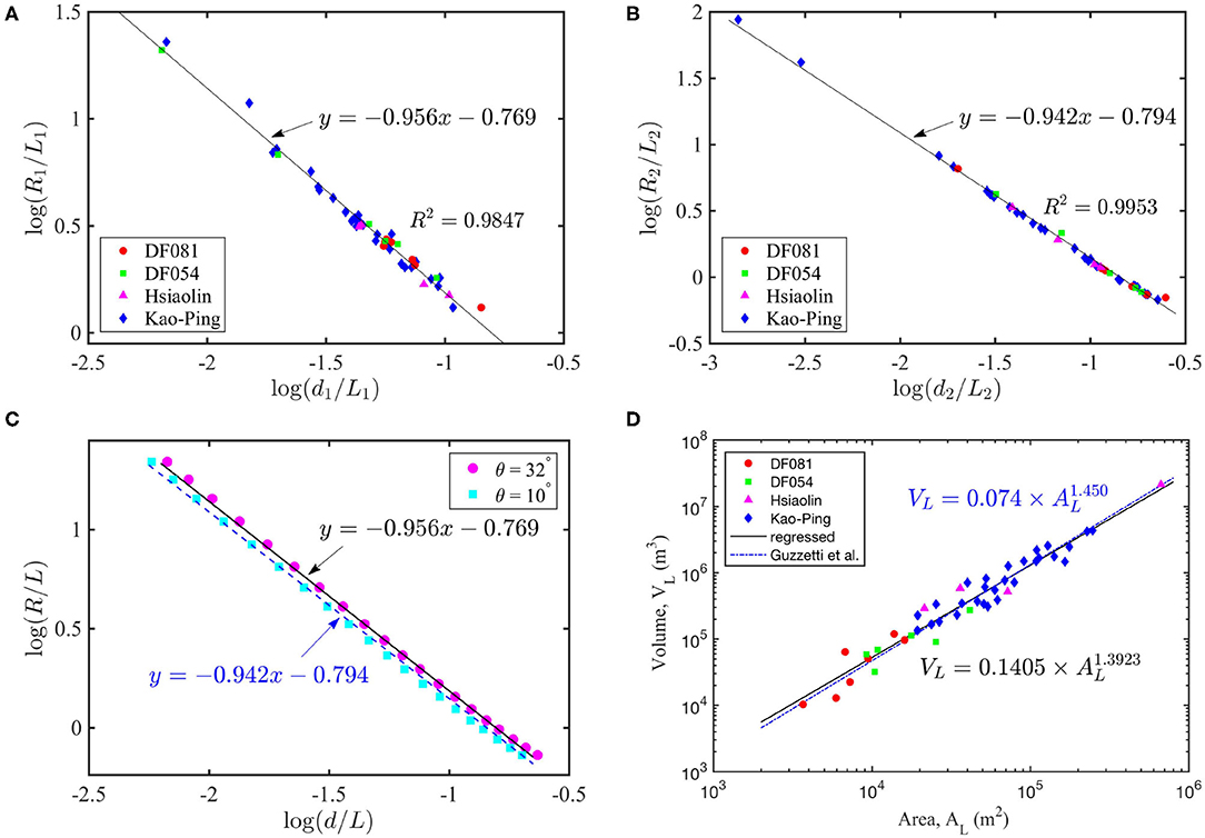
Figure 2. The specific relations among the mean curvature radius R, depth d, and length L. (A) In the down-slope axis direction; (B) In the transverse direction; (C) The ideal curves with constant inclination angles. (D) The released volume against the failure area for the analyzed, 45 landslide events, where the black solid line indicates the regressed relation (6) and the blue dash-dotted line is for the formula (5).

The specific relations, (3) and (4), may simplify the complicated iteration process of solving (2) without knowing the magnitude of θ. In using them, one should pay special attention to the definitions of d₁ and d₂ in (3) and (4). As shown in Figure 1A, $\overline{p_1{p}_2}$ and $\overline{p_3{p}_4}$ may be on different levels so that d₁ and d₂ would have distinct values with respect to a given failure depth. For an identified area of a slope failure of potential, p₁ is chosen to be at the top of the area with p₂ at the lowest point, where the line $\overline{p_3{p}_4}$ is perpendicular to the vertical section of $\overline{p_1{p}_2}$ and vertically above the midpoint p_m, see Figure 1. With respect to a given failure depth/position below the midpoint p_m (cf. Figure 1B), the values of d₁ and d₂ can be easily determined. Because L₁ and L₂ are given by the lengths of $\overline{p_1{p}_2}$ and $\overline{p_3{p}_4}$, R₁ and R₂ can, therefore, be determined with the help of (3) and (4), and the idealized failure surface is then uniquely determined.

2.3. Construction of the ICS for a Landslide-Prone Area

Until today, the ways to determine the failure depth are still open to debate. Conventionally, the failure depth is determined by the analysis of the safety factor with respect to a pre-defined failure surface (Bishop, 1955; Bishop and Morgenstern, 1960; Zheng, 2012; Das and Sivakugan, 2016). In the present study, we consider an alternative method, i.e. through the empirical relation between the source area of a landslide and its associated released volume. Since the 60's, the volume-area relation has been investigated based on individual landslides of variant types in different areas (e.g., Simonett, 1967; Rice et al., 1969; Imaizumi and Sidle, 2007; Parker et al., 2011). Guzzetti et al. (2009) analyzed 677 landslides of sliding type in Italy and suggested the representative empirical formula,

with R² = 0.9707, where A_L (in m²) stands for the area and V_L (in m³) denotes the associated landslide volume, see the blue dash-dotted line in Figure 2D. In the present study, a similar relation is proposed (see the black solid line in Figure 2D),

appropriate for the analyzed 45 landslide events (source scars) in southern Taiwan. As shown in Figure 2D, these two formulas, (5) and (6), are very close, while their reference cases lie in distinct areas. Although it has been elaborated in Larsen et al. (2010), in which 4, 231 cases were collected, that the exponent ranges from 1.1 to 1.3 for soil-based landslides and 1.3 to 1.6 for ones involving the failure of bed-rock, the similarity between (5) and (6) reveals more or less their applicability in the corresponding local area. With the help of an appropriate volume-area relation, such as (6) or (5), one may estimate the landslide volume for constructing the associated ICS, once the area that is prone to landslide is identified.

As elaborated, each failure depth (d_m in Figure 1B) uniquely defines its corresponding ICS for the identified area. Hence, the failure depth can be determined according to the estimated volume, and the method of iteration can be employed once the landslide volume is given. Figure 2D shows the volume of released mass against the failure area for the analyzed 45 landslide events (source scars), where the blue dash-dotted line indicates formula (5) and the black solid line represents relation (6). The sound agreement indicates that the empirical relation (6) or (5) together with the specific relations, (3) and (4), can be employed for determining the failure volume as well as constructing the idealized curved surface.

3. Application to Hsiaolin Landslide in Taiwan, 2009

The proposed idealized failure surface is then applied to retracing (back-calculating) the movement of a large-scale landslide event, the Hsiaolin Landslide that took place in Taiwan in 2009. The numerical simulation is performed and compared against the results computed with the post-event failure surface. In the computation, the two-phase debris model for non-trivial topography (Tai et al., 2019) is employed, where all the parameters are set identical to the ones used in Tai et al. (2019). The computational domain was 3, 700 × 2, 210 m with mesh size Δx = Δy = 10 m, and three source scars (HL-1, HL-2, and HL-3, cf. Supplementary Figure B1C) were taken into account in the computation. All the sliding masses were released simultaneously for simplicity (Kuo et al., 2011, 2013; Tai et al., 2019). Although this scenario (simultaneous release) might be highly unlikely in reality, it is a compromise for the lack of definite evidence of the release sequence, and the influence is rather minor. For the sake of brevity, we are not showing hereunder the model equations. For details on the model equations and applied parameters, the readers may refer to Tai et al. (2019).

As the idealized curved surface is a smooth surface, the calculated geometry of the initially released mass is certainly different from that calculated with respect to the post-event failure surface. In Figure 3, the released landslide mass calculated by considering the idealized curved surface (ICS) is shown in panel (A), whilst the initial landslide mass calculated with respect to the post-event failure surface (FS) is given in panel (B). The difference between these two masses is significant: the thickness discrepancy ranges from −42.58 to 59.34 m (cf. panel C or Supplementary Table C1). Moreover, the resultant scar areas are not identical and a deviation around 23% has been identified. Figure 3D illustrates the discrepancy of areas covered by the idealized curved surface (ICS) and the post-event failure surface (FS): the area in blue-green indicates the one covered both by ICS and FS; the area only occupied by the ICS is marked in golden yellow; and the blue color represents the scar area not covered by the ICS (i.e., FS only). In order to point out the size of the landslide, the Hsiaolin village is shown for scale, highlighted by the red line in Figure 3C.

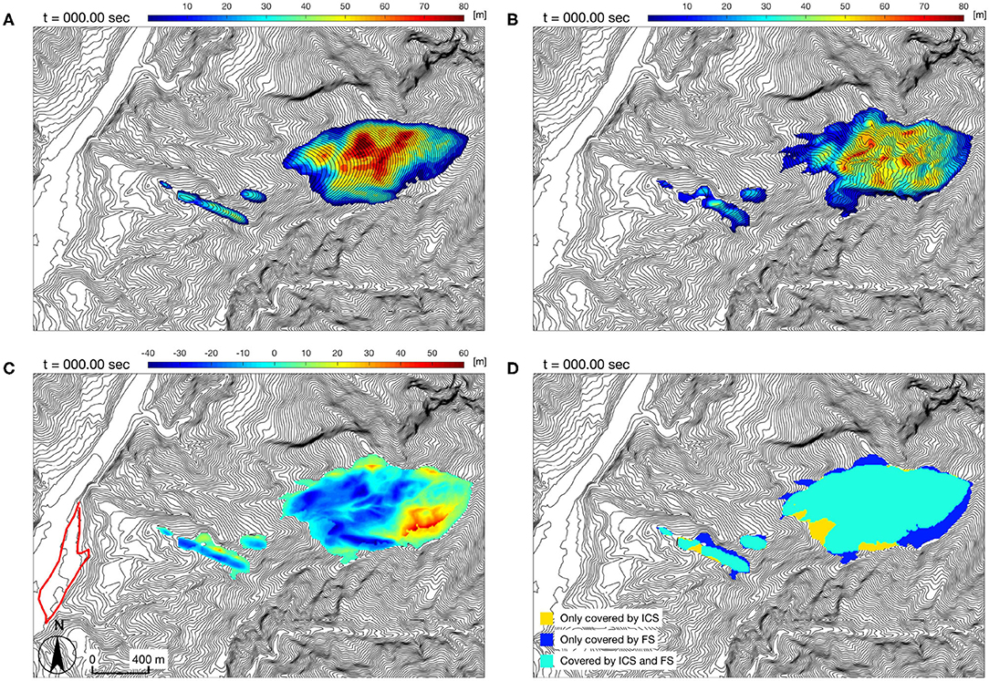
Figure 3. The geometry and thickness distribution of the initially released mass. (A) Computed with the idealized curved surface (ICS). (B) Computed with respect to the post-event failure surface (FS). (C) Thickness difference between cases a) and b), where the red line marks the location of the Hsiaolin village between the results in panels (A) and (B). (D) Covered area, where the golden yellow means the area only covered by the ICS, the blue area stands for the one only covered by FS and the blue-green area is covered by both ICS and FS.

Figure 4 illustrates the evolution of the thickness difference computed with the ICS and the FS, where the data of flow thickness <1 cm are isolated. Together with Figure 3C, the left panels of Figure 4 illustrate the differences in flow thickness at various time levels. The discrepancy of the initial thickness is significant (Figure 3C), but the difference reduces as time passes (Figures 4A,C,E). The range of difference drops from [−43.4m, 61.9m] at t = 0 s to [−16.7m, 11.7m] at t = 181.83 s (cf. the blue shade in Figure 5), when the flowing body is nearly at the state of rest. Figures 4B,D,F depict the flow paths at different moments in time. It is found that the discrepancy dramatically decreases, especially for the flow paths (flow covered area). Figure 5 summarizes the evolutions of the volume difference (green line), the discrepancy of the covered area (red line) and the depth difference (blue shaded) from t = 0 s to t = 181.83 s. As shown in Figure 5, the variation of the volume difference (green line) slightly increases, from 2.83 to 3.74%, and this increase is suspected to be caused by the outflow from the computational domain. The discrepancy of the flow paths (flow-covered area, red line) is 26.82% at t = 0.0 s and reduces to 9.48% at t = 181.83 s. The notable variation takes place at the first stage (t < 80 s), and it is supposed to be caused by the difference between the ICS and FS. For t > 75 s, the discrepancy monotonically decreases and tends to be around 9.5% at the deposition stage. Regarding the thickness difference, a significant variation of the depth difference (blue shaded) is also noted when t < 42.4 s, while the range asymptotically reduces to [−16.7, 11.7m] at t = 181.83 s. For detailed information, the data of the discrepancy evolutions are collected in Supplementary Table C1.

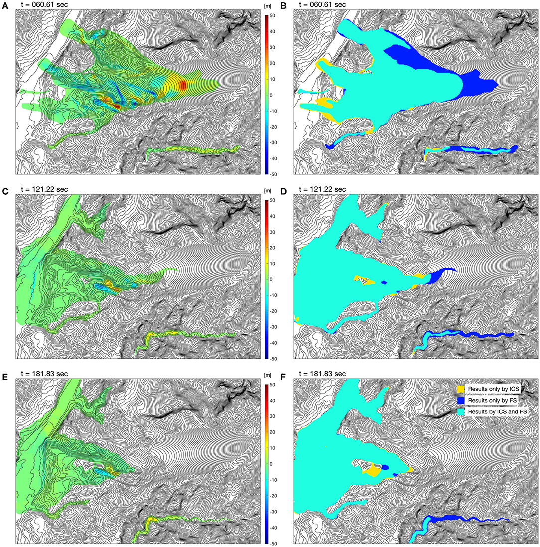
Figure 4. The thickness difference (A,C,E) and flow paths (B,D,F) of the results computed with the ICS and the FS at time levels of 60.61, 121.22, and 181.83 s, where the data of flow thickness <1 cm are isolated.

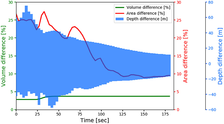
Figure 5. The evolutions of the volume difference (green line), the discrepancy of the covered area (red line), and the depth difference (blue shade) during the simulation period (from t = 0 s to t = 181.83 s).

Figure 6A is an orthophoto (satellite image) taken ca. 7 months after the Hsiaolin Landslide event, in which the bare zones approximately indicate the areas covered by the moving mass (flow paths, source scars, and deposit areas). In Figure 6B, the computed flow paths during the period of computation (from t = 0.0 s to t = 181.83 s) have been marked with respect to the satellite image, where the idealized curved surface (ICS) is employed in the computation and the area with flow thickness <1 cm is isolated. The computed flow paths are composed of 61 sets of results, i.e., with an increment of 3.0305 s, which are in sound agreement with the bare areas in the satellite image. As shown in Supplementary Table C1, the discrepancy of the flow paths between the results computed with the ICS and FS is 26.82% at the stage of initiation, causing the overflows at the northern and southern flanks of the source scar. This discrepancy reduces, as time marches, to ca. 9.5% at the stage of rest. These findings concerning the reductions of the discrepancy in flow paths and of the range of thickness difference indicate the feasibility of employing the ICS for representing the FS by retracing or predicting the plausible traveling paths, especially before the failure takes place and the slope-failure area of potential has been identified.

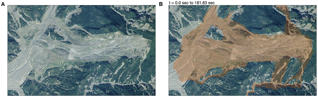
Figure 6. (A) Satellite orthophoto after the Hsiaolin Landslide event, where the bare area approximately indicates the flow paths. (B) The computed flow path covered area, where the ICS is used and the area with flow thickness <1 cm is isolated.

4. Concluding Remarks

In the present study, an idealized curved surface (ICS) is proposed to mimic the failure surface of a landslide of sliding type for the sake of performing numerical simulations. Through the investigation on historical events by means of the proposed ICS, specific relations are suggested for R/L and d/L in the down-slope and cross-slope directions. Another interesting finding is that, for the 45 source scars in southern Taiwan, the specific relation between landslide volume and area is very close to that suggested by Guzzetti et al. (2009) for landslides in Italy. These relations provide useful information for constructing the ICS. Since each failure depth d is associated with one unique ICS as well as the volume to be released, one may determine the corresponding ICS through iteration, once the landslide volume is given. For a landslide-prone area whose boundary is identified, the plausible released volume can be estimated by the empirical volume-area formula, either (5) or (6), so that the idealized sliding surface can be determined by iteration. Based on the constructed ICS, the associated plausible released volume is determined and numerical simulations can therefore be performed for the sake of hazard assessment or evaluating remediation measures.

The feasibility of the employment of the ICS is investigated through the back-calculation of a large-scale landslide with a two-phase grain-fluid model (Tai et al., 2019). The ICS is constructed with respect to the source scar and released volume given in Tai et al. (2019). Because the ICS is smooth but the FS is rather rugged, significant deviations of the flow thickness and flow paths are observed at the first stage. However, it is interesting that the discrepancy decreases as time passes and the deviations for the final shapes of the deposit are rather minor. The difference of flow-covered area drops from 26.82% (initial condition) to 9.54% at the deposition stage. In the computational period, the range of the depth difference has shrunk 73%, i.e., from [−43.4, 61.9m] to [−16.7, 11.7m]. In comparison with the post-event orthophoto, the results computed with the ICS allow to approximately retrace the flow paths as indicated in the photograph. This finding reveals that the flowing paths of a landslide are dominated by the topographic condition, such as channelization, and less sensitive to the geometry of the failure surface, especially after a long traveling distance. That is, in case the main part of the moving mass flows into a channelized topography at the first stage, the geometry of the failure surface does not play a crucial role.

It is worth pointing out that the proposed ICS does not take into account the spatial geological and hydrological variations, weathering effects, or the complex and inhomogeneous (non-isotropic) composition of the site. The current ICS is a compromise, which is not suggested for replacing those determined by the stability analysis. It only provides a plausible failure surface for a quick hazard assessment under the circumstance that no detailed local geological and hydrological condition is available. On the other hand, the current proposed ICS can provide the candidate surface for stability analysis as what has been done by Scoops3D (Reid et al., 2015), so that the hydrological condition or the local geological structure can be taken into account. That is, the ICS provides the possibility of investigating the potential area of slope failure by integrating the above mentioned hydrological condition as well as the local geological structure, which are generally of high uncertainty. With respect to the ICS, variant hydrological conditions (such as the ground-water level, distribution pattern, or seepage directions, etc.) can be applied for evaluating the associated safety factors, where failure is supposed to take place at the lowest value of the safety factor. That is to say, it enables us to retrace the plausible hydrological condition at the initiation stage for the historical landslide events. Moreover, variant scenario investigations can be performed for the purpose of hazard assessment or evaluating the countermeasure of disaster mitigation. With these, a high potential of the proposed ICS in engineering applications can be expected.

Data Availability Statement

The datasets generated for this study are available on request to the corresponding author.

Author Contributions

Y-CT: provide the idea, design the work, and construct the MS. C-YK, R-FC, and C-WL: concept/opinion exchange and ensure the contents. C-JK, K-DL, and Y-CW: perform the data analysis and numerical simulation. All authors contributed to the article and approved the submitted version.

Conflict of Interest

The authors declare that the research was conducted in the absence of any commercial or financial relationships that could be construed as a potential conflict of interest.

Acknowledgments

The financial support of the Ministry of Science and Technology, Taiwan (MOST 108-2221-E-006-015) and the Soil and Water Conservation Bureau, Council of Agriculture, Taiwan (SWCB-108-235) were acknowledged.

Supplementary Material

The Supplementary Material for this article can be found online at: https://www.frontiersin.org/articles/10.3389/feart.2020.00313/full#supplementary-material

References

Alvioli, M., Lee, G., and An, H. U. (2018). Three-dimensional, time-dependent modeling of rainfall-induced landslides over a digital landscape: a case study. Landslides 15, 1071–1084. doi: 10.1007/s10346-017-0931-7
Bishop, A. W. (1955). The use of the slip circle in the stability analysis of slopes. Geotechnique 5, 7–17. doi: 10.1680/geot.1955.5.1.7
Bishop, A. W., and Morgenstern, N. (1960). Stability coefficients for earth slopes. Geotechnique 10, 129–153. doi: 10.1680/geot.1960.10.4.129
Briaud, J.-L. (2013). Geotechnical Engineering: Unsaturated and Saturated Soils. Hoboken, NJ: John Wiley & Sons.
Bronstein, I. N., Semendjajew, K. A., Grosche, G., Ziegler, V., Ziegler, D., and Zeidler, E. (1996). Teubner-Taschenbuch der Mathematik. Leipzig: B.G. Teubner Verlagsgesellschaft Leipzig.
Chen, K.-T., Kuo, Y.-S., and Shieh, C.-L. (2014). Rapid geometry analysis for earthquake-induced and rainfall-induced landslide dams in Taiwan. J. Mount. Sci. 11, 360–370. doi: 10.1007/s11629-013-2664-y
Das, B. M., and Sivakugan, N. (2016). Fundamentals of Geotechnical Engineering. Boston, MA: Cengage Learning.
Delbridge, B. G., Bürgmann, R., Fielding, E., Hensley, S., and Schulz, W. H. (2016). Three-dimensional surface deformation derived from airborne interferometric UAVSAR: application to the Slumgullion landslide. J. Geophys. Res. Solid Earth 121, 3951–3977. doi: 10.1002/2015JB012559
Dong, J.-J., Li, Y.-S., Kuo, C.-Y., Sung, R.-T., Li, M.-H., Lee, C.-T., et al. (2011). The formation and breach of a short-lived landslide dam at Hsiaolin village, Taiwan—part I: post-event reconstruction of dam geometry. Eng. Geol. 123, 40–59. doi: 10.1016/j.enggeo.2011.04.001
Guzzetti, F., Ardizzone, F., Cardinali, M., Rossi, M., and Valigi, D. (2009). Landslide volumes and landslide mobilization rates in Umbria, central Italy. Earth Planet. Sci. Lett. 279, 222–229. doi: 10.1016/j.epsl.2009.01.005
Huang, C.-C., and Tsai, C.-C. (2000). New method for 3D and asymmetrical slope stability analysis. J. Geotech. Geoenviron. Eng. 126, 917–927. doi: 10.1061/(ASCE)1090-0241(2000)126:10(917)
Huang, C.-C., Tsai, C.-C., and Chen, Y.-H. (2002). Generalized method for three-dimensional slope stability analysis. J. Geotechn. Geoenviron. Eng. 128, 836–848. doi: 10.1061/(ASCE)1090-0241(2002)128:10(836)
Hungr, O., Leroueil, S., and Picarelli, L. (2014). The Varnes classification of landslide types, an update. Landslides 11, 167–194. doi: 10.1007/s10346-013-0436-y
Imaizumi, F., and Sidle, R. C. (2007). Linkage of sediment supply and transport processes in Miyagawa Dam catchment, Japan. J. Geophys. Res. Earth Surf. 112:F03012. doi: 10.1029/2006JF000495
Iverson, R. M., George, D. L., Allstadt, K., Reid, M. E., Collins, B. D., Vallance, J. W., et al. (2015). Landslide mobility and hazards: implications of the 2014 Oso disaster. Earth Planet. Sci. Lett. 412, 197–208. doi: 10.1016/j.epsl.2014.12.020
Jaboyedoff, M., Baillifard, F., Couture, R., Locat, J., and Locat, P. (2004). “Toward preliminary hazard assessment using DEM topographic analysis and simple mechanic modeling,” in Landslides: Evaluation and Stabilization, eds W. A. Lacerda, M. Ehrlich, S. A. B. Fontoura, A. S. Sayao (London: Taylor and Francis Group), 199–206.
Jaboyedoff, M., Couture, R., and Locat, P. (2009). Structural analysis of Turtle Mountain (Alberta) using digital elevation model: toward a progressive failure. Geomorphology 103, 5–16. doi: 10.1016/j.geomorph.2008.04.012
Kuo, C.-Y., Tai, Y.-C., Bouchut, F., Mangeney, A., Pelanti, M., Chen, R.-F., et al. (2009). Simulation of Tsaoling landslide, Taiwan, based on Saint-Venant equations over general topography. Eng. Geol. 104, 181–189. doi: 10.1016/j.enggeo.2008.10.003
Kuo, C.-Y., Tai, Y.-C., Chen, C.-C., Chang, K.-J., Siau, A.-Y., Dong, J.-J., et al. (2011). The landslide stage of the Hsiaolin catastrophe: simulation and validation. J. Geophys. Res. Earth Surf. 116:F04007. doi: 10.1029/2010JF001921
Kuo, C.-Y., Tsai, P.-W., Tai, Y.-C., Chan, Y.-H., Chen, R.-F., and Lin, C.-W. (2020). Application assessments of using scarp boundary-fitted, volume constrained, smooth minimal surfaces as failure interfaces of deep-seated landslides. Front. Earth Sci. 8:211. doi: 10.3389/feart.2020.00211
Kuo, Y.-S., Tsai, Y.-J., Chen, Y.-S., Shieh, C.-L., Miyamoto, K., and Itoh, T. (2013). Movement of deep-seated rainfall-induced landslide at Shiaolin Village during Typhoon Morakot. Landslides 10, 191–202. doi: 10.1007/s10346-012-0315-y
Lam, L., and Fredlund, D. (1993). A general limit equilibrium model for three-dimensional slope stability analysis. Can. Geotech. J. 30, 905–919. doi: 10.1139/t93-089
Larsen, I. J., Montgomery, D. R., and Korup, O. (2010). Landslide erosion controlled by hillslope material. Nat. Geosci. 3, 247–251. doi: 10.1038/ngeo776
Lin, C.-W., Chang, W.-S., Liu, S.-H., Tsai, T.-T., Lee, S.-P., Tsang, Y.-C., et al. (2011). Landslides triggered by the 7 August 2009 typhoon Morakot in southern Taiwan. Eng. Geol. 123, 3–12. doi: 10.1016/j.enggeo.2011.06.007
Lin, C.-W., Tseng, C.-M., and Chen, R.-F. (2013). Survey and Assessment of Potential Large-Scale Landslides Hazards in Mountainous Areas of Kao-Ping River Watershed. Technical report, Soil and Water Conservative Bureau, Council of Agriculture, Nantou, Taiwan.
Lin, M.-L., Chen, T.-W., Lin, C.-W., Ho, D.-J., Cheng, K.-P., Yin, H.-Y., et al. (2014). Detecting large-scale landslides using LiDar data and aerial photos in the Namasha-Liuoguey area, Taiwan. Rem. Sens. 6, 42–63. doi: 10.3390/rs6010042
Lo, C.-M., Lin, M.-L., Tang, C.-L., and Hu, J.-C. (2011). A kinematic model of the Hsiaolin Landslide calibrated to the morphology of the landslide deposit. Eng. Geol. 123, 22–39. doi: 10.1016/j.enggeo.2011.07.002
Manzella, I., and Labiouse, V. (2013). Empirical and analytical analyses of laboratory granular flows to investigate rock avalanche propagation. Landslides 10, 23–36. doi: 10.1007/s10346-011-0313-5
Mergili, M., Jaboyedoff, M., Pullarello, J., and Pudasaini, S. P. (2020). Back calculation of the 2017 Piz Cengalo-Bondo landslide cascade with r.avaflow: what we can do and what we can learn. Nat. Hazards Earth Syst. Sci. 20, 505–520. doi: 10.5194/nhess-20-505-2020
Parker, R. N., Densmore, A. L., Rosser, N. J., De Michele, M., Li, Y., Huang, R., et al. (2011). Mass wasting triggered by the 2008 Wenchuan earthquake is greater than orogenic growth. Nat. Geosci. 4, 449–452. doi: 10.1038/ngeo1154
Reid, M. E., Christian, S. B., and Brien, D. L. (2000). Gravitational stability of three-dimensional stratovolcano edifices. J. Geophys. Res. Solid Earth 105, 6043–6056. doi: 10.1029/1999JB900310
Reid, M. E., Christian, S. B., Brien, D. L., and Henderson, S. (2015). Scoops3D-Software to Analyze Three-Dimensional Slope Stability Throughout a Digital Landscape. Menlo Park, CA: US Geological Survey; Volcano Science Center.
Reid, M. E., Sisson, T. W., and Brien, D. L. (2001). Volcano collapse promoted by hydrothermal alteration and edifice shape, Mount Rainier, Washington. Geology 29, 779–782. doi: 10.1130/0091-7613(2001)029<0779:VCPBHA>2.0.CO;2
Rice, R. M., Crobett, E., and Bailey, R. (1969). Soil slips related to vegetation, topography, and soil in southern California. Water Resour. Res. 5, 647–659. doi: 10.1029/WR005i003p00647
Scheidegger, A. E. (1973). On the prediction of the reach and velocity of catastrophic landslides. Rock Mech. 5, 231–236. doi: 10.1007/BF01301796
Simonett, D. S. (1967). “Landslide distribution and earthquakes in the Bavani and Torricelli Mountains, New Guinea,” in Landform Studies from Australia and New Guinea, eds J. N. Jennings and J. A. Mabbutt (Cambridge: Cambridge University Press), 64–84.
Song, Y., Huang, D., and Zeng, B. (2017). GPU-based parallel computation for discontinuous deformation analysis (DDA) method and its application to modelling earthquake-induced landslide. Comput. Geotech. 86, 80–94. doi: 10.1016/j.compgeo.2017.01.001
Stumpf, A., Malet, J.-P., Kerle, N., Niethammer, U., and Rothmund, S. (2013). Image-based mapping of surface fissures for the investigation of landslide dynamics. Geomorphology 186, 12–27. doi: 10.1016/j.geomorph.2012.12.010
Tai, Y.-C., Heß, J., and Wang, Y. (2019). Modeling two-phase debris flows with grain-fluid separation over rugged topography: application to the 2009 Hsiaolin event, Taiwan. J. Geophys. Res. Earth Surf. 124, 305–333. doi: 10.1029/2018JF004671
Tai, Y.-C., and Jan, C.-D. (2019). Advanced Study on the Algorithm for Plausibly Estimating the Amount of Landslide Mass and Its Traveling Path. Technical report, Soil and Water Conservative Bureau, Council of Agriculture, Nantou, Taiwan.
Tsou, C.-Y., Feng, Z.-Y., and Chigira, M. (2011). Catastrophic landslide induced by typhoon Morakot, Shiaolin, Taiwan. Geomorphology 127, 166–178. doi: 10.1016/j.geomorph.2010.12.013
Wu, J.-H. (2010). Seismic landslide simulations in discontinuous deformation analysis. Comput. Geotech. 37, 594–601. doi: 10.1016/j.compgeo.2010.03.007
Yu, P., Zhang, Y., Peng, X., Wang, J., Chen, G., and Zhao, J. X. (2019). Evaluation of impact force of rock landslides acting on structures using discontinuous deformation analysis. Comput. Geotech. 114:103137. doi: 10.1016/j.compgeo.2019.103137
Zhan, W., Fan, X., Huang, R., Pei, X., Xu, Q., and Li, W. (2017). Empirical prediction for travel distance of channelized rock avalanches in the wenchuan earthquake area. Nat. Hazards Earth Syst. Sci. 17, 833–844. doi: 10.5194/nhess-17-833-2017
Zhang, L., Li, J., Li, X., Zhang, J., and Zhu, H. (2018). Rainfall-Induced Soil Slope Failure: Stability Analysis and Probabilistic Assessment. Boca Raton, FL: CRC Press.
Zhang, S., and Wang, F. (2019). Three-dimensional seismic slope stability assessment with the application of Scoops3D and GIS: a case study in Atsuma, Hokkaido. Geoenviron. Disast. 6:9. doi: 10.1186/s40677-019-0125-9
Keywords: landslide, slope failure, failure surface, idealized curved surface (ICS), flow paths, hazard assessment
Citation: Tai Y-C, Ko C-J, Li K-D, Wu Y-C, Kuo C-Y, Chen R-F and Lin C-W (2020) An Idealized Landslide Failure Surface and Its Impacts on the Traveling Paths. Front. Earth Sci. 8:313. doi: 10.3389/feart.2020.00313
Received: 29 February 2020; Accepted: 02 July 2020;
Published: 21 August 2020.
Edited by:
Yosuke Aoki, The University of Tokyo, JapanReviewed by:
Federico Pasquaré Mariotto, University of Insubria, ItalyScott McDougall, University of British Columbia, Canada
Copyright © 2020 Tai, Ko, Li, Wu, Kuo, Chen and Lin. This is an open-access article distributed under the terms of the Creative Commons Attribution License (CC BY). The use, distribution or reproduction in other forums is permitted, provided the original author(s) and the copyright owner(s) are credited and that the original publication in this journal is cited, in accordance with accepted academic practice. No use, distribution or reproduction is permitted which does not comply with these terms.
*Correspondence: Yih-Chin Tai, yctai@mail.ncku.edu.tw