the Creative Commons Attribution 4.0 License.
the Creative Commons Attribution 4.0 License.
 | 16 Jul 2020
Signal processing for in situ detection of effective heat pulse probe spacing radius as the basis of a self-calibrating heat pulse probe
John W. Pomeroy
A sensor comprised of an electronic circuit and a hybrid single and dual heat pulse probe was constructed and tested along with a novel signal processing procedure to determine changes in the effective dual-probe spacing radius over the time of measurement. The circuit utilized a proportional–integral–derivative (PID) controller to control heat inputs into the soil medium in lieu of a variable resistor. The system was designed for onboard signal processing and implemented USB, RS-232, and SDI-12 interfaces for machine-to-machine (M2M) exchange of data, thereby enabling heat inputs to be adjusted to soil conditions and data availability shortly after the time of experiment. Signal processing was introduced to provide a simplified single-probe model to determine thermal conductivity instead of reliance on late-time logarithmic curve fitting. Homomorphic and derivative filters were used with a dual-probe model to detect changes in the effective probe spacing radius over the time of experiment to compensate for physical changes in radius as well as model and experimental error. Theoretical constraints were developed for an efficient inverse of the exponential integral on an embedded system. Application of the signal processing to experiments on sand and peat improved the estimates of soil water content and bulk density compared to methods of curve fitting nominally used for heat pulse probe experiments. Applications of the technology may be especially useful for soil and environmental conditions under which effective changes in probe spacing radius need to be detected and compensated for over the time of experiment.
- Article
(4623 KB) - Full-text XML
- BibTeX
- EndNote


The heat pulse probe (HPP) is widely used to determine the thermal conductivity (Abu-Hamdeh, 2001; Abu-Hamdeh and Reeder, 2000; Jin et al., 2017; Li et al., 2016; Liu et al., 2007; Ochsner and Baker, 2008; Penner, 1970; Yun and Santamarina, 2008), thermal diffusivity, and heat capacity (Bristow, 1998; Ham and Benson, 2004; Kluitenberg et al., 1993; Liu et al., 2007; Ochsner et al., 2001; Zhang et al., 2014) of soil. HPPs have been used to measure the thermal conductivity (Morin et al., 2010; Sturm and Johnson, 1992) and density of snow (Liu and Si, 2008); a review is presented by Kinar and Pomeroy (2015). For soils, HPP measurements provide inputs for mathematical models used to determine volumetric water content (Basinger et al., 2003; Bristow, 1998; Bristow et al., 1993; Ham and Benson, 2004; Heitman et al., 2003; Li et al., 2016; Song et al., 1998) and water flux (Hopmans et al., 2002; Kamai et al., 2008; Mori et al., 2003; Wang et al., 2002). A comprehensive review of HPP sensors used to measure water flux is given by He et al. (2018). Installed into a tree trunk (Green et al., 2003) or plant stem (Miner et al., 2017), HPPs can measure sap flow rates. Multifunctional HPPs can simultaneously measure soil thermal and electrical properties to determine soil water retention and hydraulic conductivity (Bristow et al., 2001; Mori et al., 2003; Valente et al., 2006). Data from HPPs can be used to drive predictive mathematical models for water transport (Liu and Si, 2008; Saito et al., 2006; Trautz et al., 2014) and snowpack evolution (Ochsner and Baker, 2008). These models are also useful for civil and geological engineering applications (Ochsner et al., 2001), as well as for prediction of runoff (Yang and Jones, 2009), agricultural productivity (Pearsall et al., 2014; Sturm and Johnson, 1992), climate change, and avalanche hazards (Morin et al., 2010).
HPPs can be broadly classified into two different types: single-probe (SP) (De Vries, 1952; Li et al., 2016) and dual-probe (DP) (Bristow et al., 1993; Campbell et al., 1991; Ham and Benson, 2004) devices. The SP consists of a single heater needle that is inserted into the geomaterial. A temperature measurement sensor (i.e., a thermistor) placed inside the heater needle is used to determine the change in temperature as the needle releases thermal energy. The DP consists of two needles that are inserted into the geomaterial: one of the needles functions as a heater, whereas the other needle measures the change in temperature of the geomaterial at an offset distance to the heated needle. The DP has an advantage over the SP since the SP can only be used to determine thermal conductivity, whereas the DP can be used to determine the thermal conductivity and diffusivity of the geomaterial (Bristow et al., 1994).
An assumption nominally made in conjunction with DP sensors is that the radius is constant during each measurement. If the DP radius changes after the probe is inserted into the geomaterial or over the time of measurement due to heating and cooling, HPP determination of thermal properties will be inaccurate (Kluitenberg et al., 1993; Mori et al., 2003). The measured thermal conductivity is not sensitive to changes in DP probe spacing radius, whereas the HPP-determined heat capacity and thermal diffusivity exhibit high sensitivity to radius changes (Kluitenberg et al., 2010; Liu et al., 2007). This creates challenges in estimating the moisture content of frozen soils wherein thawing and freezing occur and has required recalibration of individual probes (Zhang et al., 2011).
Most HPP researchers utilized commercially available off-the-shelf (COTS) hardware (i.e., a datalogger) to collect data (Bristow, 1998; Bristow et al., 1994, 2001; Kamai et al., 2008; Li et al., 2016), although recently custom electronic circuits have been proposed. Valente et al. (2006) interfaced a multifunctional soil probe to a processing circuit. Dias et al. (2013) used an NPN transistor as a heat source for an SP device. The temperature of the transistor was determined using a circuit and transistor circuit theory. Sherfy et al. (2016) used an NE555 timer circuit to control the duration of the heating pulse. Miner et al. (2017) and Ravazzani (2017) developed Arduino-based HPP sensors utilizing currently established DP theory. Liu et al. (2013), Wen et al. (2015), and Liu et al. (2016) showed that two or more thermistors placed inside the temperature measurement needles of a DP device can be used to determine probe deflection. Multiple thermistors are required to determine probe deflection, and the method cannot be used to calculate a time series of small changes in the probe spacing radius that occur during the time of measurement when the heater needle increases in temperature.
A self-calibrating heat pulse probe (SCHEPP) system is described that consists of a custom electronic circuit and novel inverse models for the SP and DP. The HPP used for SCHEPP is a hybrid of the SP and DP designs. SP and DP forward models are combined and used to determine changes in the effective probe spacing radius during the time of measurement. This effective radius compensates for model error and, similar to a calibrated probe spacing radius, does not directly coincide with the actual probe spacing radius. Another inverse model is also introduced that allows for the determination of thermal conductivity without the need for an SP model late-time approximation (see Sect. 2.2.1 for the rationale).
Diagrams of the SCHEPP system HPP are shown as Figs. 1a and 2a. A loop of nichrome wire is placed inside a heater needle, along with a measurement thermistor. Another measurement thermistor is placed inside a temperature-sensing needle situated at an offset distance to the heater needle. Figure 2a shows that SCHEPP uses a hybrid SP and DP device. A proportional–integral–derivative (PID) controller is used to precisely control and maintain heat inputs in lieu of a variable resistor. Circuit theory is used to determine the resistance of the nichrome heating wire inside the heater needle during a measurement. This eliminates the need to use a previously measured estimate of the heater wire resistance. The heater wire resistance is directly measured over the time of an experiment. Figure 1b is a conceptual diagram that shows relationships between the models and measurement methods.
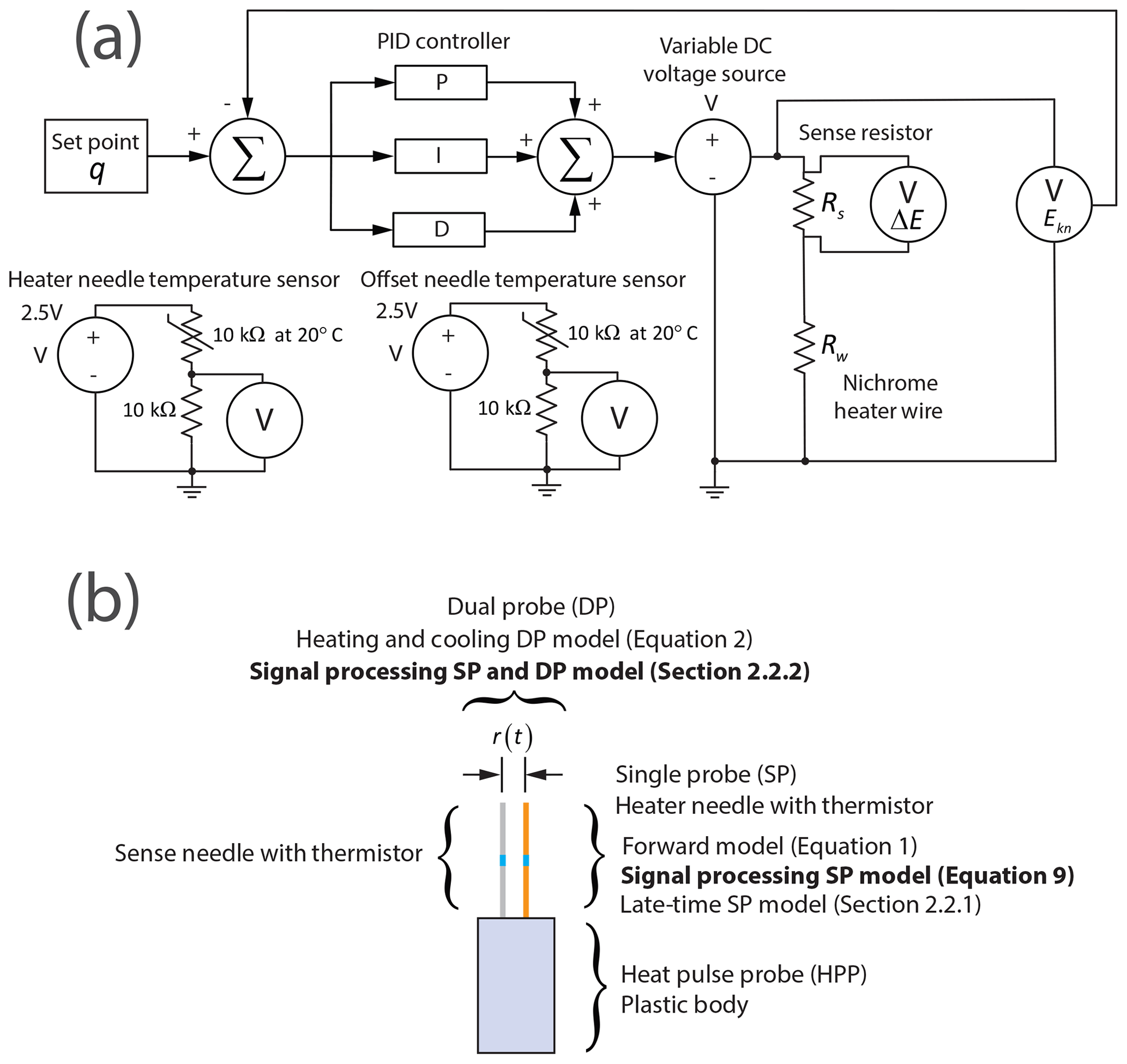
Figure 1(a) Conceptual block diagram of the HPP system. The set point q and the PID controller ensure a constant input of heat into the soil over the length of the heater needle. The PID controller modulates heat inputs by changing the output of a variable DC voltage source, and the feedback path is shown. A Kelvin-connection sense resistor measures the current through the nichrome heater wire. A reduction in voltage over the sense resistor element is ΔE, and the ground-referenced output voltage through the nichrome wire is Ekn. The heater needle temperature sensor and offset needle temperature sensor circuits are also shown. A constant voltage source of 2.5 V is connected to a half-bridge. One element of the bridge is a thermistor with a nominal resistance of 10 kΩ specified at a temperature of 20 ∘C, and the other is a precision resistor with a fixed resistance. (b) Conceptual diagram showing relationships between models and heat pulse probe (HPP) measurements for the hybrid single and dual probe. Each model in the diagram is described in the associated text. Model text in bold indicates signal processing introduced in this paper. The r(t) indicates a time-variable effective radius.

Figure 2Diagrams showing the system and microcontroller. (a) The circuit operation is controlled by a 32 bit microcontroller clocked at 300 MHz by a PLL. The microcontroller and associated transceiver circuity implement M2M communications whereby data and system operation can be exchanged between machines using commands sent over USB, RS-232, or SDI-12. The microcontroller acts as a state machine that samples data from the AFE and stores the data in SDRAM where signal processing is conducted. The circuit is powered by a nominal 12 V DC supply that is reduced to 3.3 V by a DC–DC switcher. The HPP is a hybrid SP and DP design comprised of a heater needle and a sense needle. The effective distance between the needles as a function of time is r(t). (b) Picture of the circuit. (c) Soil column used in the experiment. (d) Experimental setup. (e) Image of needle probe prototype.
2.1 Forward models
Assuming that the heater needle is an infinite line source in an infinite medium, the “late-time” change in temperature ΔΓ1(t) of the heater probe SP device is given by Eq. (22a) of Blackwell (1954):
In Eq. (1) above, q is the rate of energy transferred per unit length of the probe, k is the thermal conductivity of the geomaterial, B, C, and D are constants, and the natural logarithm is utilized. The assumption of an infinite line source in an infinite medium is valid if the heater needle has a small diameter and the geomaterial is of sufficiently large dimension to be isotropic and homogeneous throughout so that the heat pulse does not interact with dissimilar boundaries (i.e., a container in which the soil is placed) over the time of the measurement (Kluitenberg et al., 1993, 1995; Liu et al., 2007). For , where rn is the radius of the needle and α is the thermal diffusivity of the medium, the last term in Eq. (1) can be neglected (Bristow et al., 1994; Li et al., 2016). In this paper, Eq. (1) as a forward model is taken subject to the constraint that ΔΓ1(t)>0 since negative values are not physically reasonable within the context of the model.
Assuming an infinite line source in an infinite medium for a DP device, the change in temperature γ1(r,t) sensed at a radial distance r from the heater needle is as follows (Kluitenberg et al., 1993).
The thermal diffusivity of the medium is α, the density is ρ, and the specific heat capacity is c. The exponential integral function is Ei. The current through the nichrome wire is turned on at time t0 and turned off at time th. Therefore, is referred to as the heating period and t>th as the cooling period. Calibration to determine a radius using least-squares curve fitting will yield an effective radius that is representative of differences between the sensing system and the ideal model described above. This initial radius is referred to as rinitial and is taken as a constant.
2.2 Inverse models
2.2.1 Thermal conductivity
Curve fitting using Eq. (1) can be conducted for the section of the heating curve where . However, the late-time approximation with increases the time of measurement and necessitates that the 1∕t term is negligible. When and for suitable t such that the model of Eq. (1) is valid, the constants are difficult to directly determine using curve fitting by optimization whereby multiple values can be found to appropriately fit the same model of Eq. (1).
Given these disadvantages, this section introduces a method, the signal processing SP model, which uses signal processing to reduce the time series associated with Eq. (1) to a simpler model. Least-squares curve fitting is used with a modified version of Eq. (1) and the total SP dataset during heating. Errors introduced during the earlier time of heating are acceptably small, particularly when signal processing has modified the SP dataset as a time-domain signal and k is obtained by a least-squares curve fit.
Equation (1) is subjected to Hadamard (point-by-point) multiplication by t to obtain
The Hadamard multiplication to produce Eq. (6) is a type of homodyning process whereby later-time values of ΔΓ1(t) are assigned greater-magnitude weights than earlier-time values. Taking the numerical time derivative is similar to the application of a high-pass filter (Hamming, 1983; pg. 118). The resulting equation is
Homodyning again by t yields
Taking the numerical time derivative again,
To reduce noise associated with the derivative operation when working with actual data, a Butterworth low-pass filter with zero-phase filtering and a cutoff frequency of 0.3 Hz is applied to the numerical sequence associated with Eq. (9). The cutoff frequency was chosen to ensure stability of the inverse model within the context of the data used for the experiments reported in this paper. Given a known q, curve fitting is applied to the filtered sequence associated with Eq. (9) to determine k without the need to also determine {C,D} at time , where the model of Eq. (1) is still valid. Once the thermal conductivity k is determined by the signal processing, curve fitting using Eq. (1) with a starting value of the determined thermal conductivity is used to estimate parameters for the application of the SP forward model.
The late-time SP model is used for comparison with the signal processing SP model described above. A linear section of the ΔΓ1(t)−log (t) curve is identified as the time td that is 1 s after the time when the second numerical derivative of the ΔΓ1(t)−log (t) curve is approximately equal to zero. The time td is identified using a signal processing zero-crossing detector, and the 1 s delay is introduced to ensure that the curve is approximately linear. Curve fitting using Eq. (1) with is then used to determine k from the linear section of the ΔΓ1(t)−log (t) curve (Li et al., 2016).
2.2.2 Dual probe and variable radius
The inverse model described in this section uses signal processing to determine r(t) as an effective radius that changes over the time of heating and cooling to compensate for model error and physical changes in the probe spacing. A numerical value for rinitial is required as an estimate of the initial probe spacing radius. Changes in the effective probe spacing r(t) are determined over time and used to obtain an α that is representative of these changes. This is the signal processing DP model.
Thermal conductivity, k, is determined using a measured q and the inverse signal processing model presented in Sect. 2.2.1 for the SP. The thermal conductivity is not directly determined from the DP model using curve fitting since the effective radius r(t) can change over time.
The k is used with a known q to algebraically remove the q∕4πk term from Eq. (2) to obtain γ2(r(t),t) as an expression written only in terms of Ei. The inverse of the exponential integral is determined using the procedure in Appendix A suitable for an embedded system.
From the inverse, we determine
The square root function transforms Eqs. (11) and (12) below. To ensure the application of the square root function with real numbers, the numerical implementation must ensure .
Taking the logarithm of Eq. (12) results in Eq. (13) below. Applied to each element of the corresponding sequence, this operation is analogous to homomorphic filtering (Oppenheim et al., 1976).
Taking the time derivative of Eq. (13) is once again similar to the application of a high-pass filter that suppresses the constant log (2α1∕2) term. When Eq. (14) is expressed as a discrete sequence sampled at a frequency of fs the derivative is approximated using a backward-difference method (Eq. 15).
The derivative is computed using a backward difference:
In Eq. (15) above, ai=log (r(ti)), where the index i denotes the element of a discrete sequence and Δt is the time step calculated by . To reduce numerical error at small time t values, the inverse model described in this section is applied with a time step Δt such that the numerical inverse of Ei(x) can be successfully computed (Sect. 2.5).
The solution of Eq. (15) requires a boundary condition ab=log (r(tinitial)), where tinitial is the time at which the probe spacing radius is rinitial. For application to actual data, we assume that the probe spacing is the calibrated rinitial at , where tp is the time at which the curve associated with γ1(r,t) is at a maximum and ta is an additional time delay that compensates for a nonideal system. For this system, the additional time delay was chosen such that . Selection of a peak time is a similar idea to the temperature maximum method (Bristow et al., 2001) whereby the calibrated rinitial is used at the time of peak temperature change. The additional time delay ta is chosen to approximately coincide with the integer-valued time durations of moving-average windows (Sect. 2.5). The input data are trimmed appropriately. This selection of boundary condition is supported by tests on actual soil performed in this paper and a sensitivity analysis that justifies the selection of the additional time ta (Sect. 3.3).
After r(t) is determined, the α is determined by taking the average of γ8(r(t),t) over time. Evaluation of Eq. (16) will thereby yield a curve that is a straight line with a slope that is approximately zero when α is approximately constant over the time of heating and cooling. The r(t) is an effective radius that is also affected by temperature drift and deviation of the physical system from an ideal model. Since r(t) is an effective radius, it will not directly coincide with an actual probe spacing radius.
2.3 Measurement of soil water content and density
The heat capacity k and thermal diffusivity α are determined using an inverse model as described in the previous sections of this paper. Neglecting the contribution of air, the volumetric heat capacity of soil Ch is calculated by Kluitenberg (2002):
Rearranging Eq. (17) and solving for volumetric water content yields the following.
In the equations above, Cm, Co, and Cw are the volumetric heat capacities of mineral content, organic content, and water; θm, θo, and θw are the associated volume fractions; and Ch is the total volumetric heat capacity of the soil. The cm and co are the specific heat capacities of the mineral and organic content, and the ρm and ρo are the associated densities. Experiments in which numerical values of θw<0 or θw>1 are not valid and indicate improper contact between the probe and the soil medium. The θw is numerically constrained to be within the range . The mineral content of the soil θm is known, and the organic content θo can be easily determined from laboratory testing or an organic carbon soil map of a geographic area. For implementation using a microcontroller, θm and θo are stored in flash (non-volatile) memory, and these values change based on the geographic location of the soil. The density of the soil is determined by volume fractions:
In Eq. (19) above, the constituent densities and heat capacities are known. The θw is determined using Eq. (18).
2.4 Circuit theory and PID control
Figure 1 shows a conceptual block diagram of the system. Thermistors in half-bridge configurations are used to determine the temperatures of HPP needles.
The heat input into the soil by the heater probe is
In the above Eqs. (20) and (21), the electrical power is P, the total resistance of the nichrome heater wire is Rw, and ℓ is the length of the heater needle. Given a measured voltage drop ΔE over a four-terminal Kelvin sense resistor with known resistance Rs, the current though the heater wire is calculated using Ohm's law:
For a current I through the heater wire and sense resistor, the output voltage is measured as Ekn by an analog-to-digital converter (Fig. 1). Using Kirchhoff's voltage law for this circuit, the resistance Rw of the nichrome wire is determined at each sampling time step by
To set a constant q, a proportional–integral–derivative (PID) controller (Ang et al., 2005) is utilized. The variable voltage source is adjusted at each discrete time step by a digital-to-analog-converter (DAC). Since ΔE and Ekn are measured at each discrete time step at a sampling rate of fs, Eqs. (20) to (23) are used with the feedback loop shown in Fig. 1 to ensure that the q remains close to a set-point value during the time of experiment. The use of the PID controller requires a higher sampling rate fs than a nominal HPP experiment to adjust the output q. The PID controller thereby ensures that the soil can heat up in a controlled fashion and considers resistance changes in the nichrome wire in lieu of using an assumed resistance. Figure 2a is a block diagram indicating how the system incorporates a microcontroller and communication interfaces.
2.5 Determination of temperature change curves
The sampled temperature inside the heater needle is denoted as Γ(t), and the sampled temperature inside the second needle at an offset distance from the heater needle is denoted as T(t). The sampled temperatures Γ(t) and T(t) are low-pass filtered using a fifth-order Butterworth filter with a cutoff frequency of 10 Hz applied as a zero-phase filter to reduce noise. The Butterworth filter was chosen since it is maximally flat in the passband, and the zero-phase filtering ensures that time shifts are minimized to ensure accurate application of the inverse models described in this paper using the collected data.
For the DP model calibration to find an initial r0 using curve fitting, the sampled temperatures are processed by a moving-average filter over 1 s windows to further reduce noise before curve fitting. Alternately, for the DP inverse model (Sect. 2.2.2), a moving-average filter is used to obtain an equivalent sampling rate of 12 Hz to ensure that the Ei(x) inverse can be accurately computed using floating-point number representations.
The respective averaged initial temperatures of the needles before heating are determined as Γav and Tav. Therefore, the temperature changes are calculated as and after the application of any initial filtering. The temperature changes are used for the application of inverse models related to Eqs. (1) and (2).
2.6 Determination of heat inputs
Heat inputs into the soil are determined during the time of experiment and calculated using Eq. (21). When the current is applied and travels through the heater wire, there is a short time delay (≪1 s) before the set point q is attained when the heater needle increases in temperature. The interval of the time series for a constant calculated q during the time of experiment is determined using a step detection algorithm (Carter et al., 2008) based on the Student's t test (Ebdon, 1991; pp. 61–64) with a null hypothesis at a significance level of 1 % and a window size of 31 elements. The significance level and window size are dependent on the implementation of the sampling system and are thereby chosen to detect the step within the context of this experiment. To find an estimate of a constant value of q, the time series is averaged over the plateau of the step. The time series location of the step associated with a constant q is found by application of a sliding mean filter with a window size of 31 elements applied to a time series of electrical power P used for the computation of q using Eq. (21). The mean filter is applied to a binary sequence created by mapping non-rejection of the null hypothesis to binary 0 and rejection of the null hypothesis to binary 1. The plateau is coincident with a sequence of zeros away from the edges of the step. The edges of the step are indicated by nonzero elements in this sequence surrounded by zeros. The window size is appropriate for the sampling system described in the context of this paper.
2.7 Apparatus
A custom electronic circuit board was designed and constructed for the SCHEPP system (Fig. 2a and b). The circuit board was placed into an enclosure box and connected to the HPP by a cable and mating circular connectors. The HPP body was epoxied into a circular hole cut in the bottom of a cylindrical polyvinyl chloride (PVC) container of 10.0 cm diameter and 10.5 cm height that held 825 cm3 of soil. The HPP needles thereby protruded into the soil column formed by the PVC container (Fig. 2c).
Figures 1 and 2a graphically show the different subsystems of the PCB (Fig. 2b). In the analog front end (AFE), a two-channel 24 bit ADC with a precision 10 k (0.01 %, ± 5 ppm ∘C) resistor half-bridge for each channel and a 2.5 V voltage reference (2 ppm ∘C, ± 0.02 % voltage error) was used to determine the resistance of the thermistors inside each needle. The resistance of a thermistor was related to temperature by the Steinhart–Hart equation (Steinhart and Hart, 1968).
The variable voltage source was constructed from a DC–DC switcher for efficiency and thereby reduced power consumption in lieu of a linear regulator. The DC–DC switcher could be turned off for an output voltage of 0 V or turned on and adjusted from ∼ 0.49 to ∼ 8.965 V using a DAC that injected current into the feedback loop of the switcher. With design criteria including a heater needle length of ℓ=3.0 cm and a nichrome wire resistance of Rw≈34 Ω, the heater output was limited by software to be within the range of q≈0.24 to . The precision sense resistor was chosen as Rs=0.01 Ω (0.1 %, ± 15 ppm ∘C) to reduce the voltage drop over this circuit element and to ensure that the output voltage could be accurately adjusted. This resistance is smaller than the 1 Ω current sense resistor nominally used in other HPP experiments (Bristow et al., 1994; Li et al., 2016; Liu and Si, 2011, 2008; Valente et al., 2006; Zhang et al., 2011). Moreover, the precision sense resistor had a Kelvin terminal connection for precision and was physically large to reduce self-heating by current flow. The voltage drop over a sense resistor was determined by a precision difference amplifier and a 16 bit ADC, allowing for a 1 LSB step size of 2.5 µV. The output voltage Ekn (Fig. 1) was also measured by a 16 bit ADC and amplifier, resulting in a 1 LSB step size of 1.25 mV.
A 32 bit microcontroller with a system clock of 300 MHz was used to control the HPP experiment and perform floating-point calculations (Fig. 2a). The system clock had to be set at 300 MHz to allow the microcontroller to sample all ADCs in the system at fs=120 Hz and also perform floating-point calculations associated with this application. The system clock speed is provided here to provide a starting point for engineering of similar designs. The DAC used to control the output voltage was also updated at the same sampling rate with the PID controller output. The 120 Hz sampling rate enabled functioning of the PID controller feedback loop and allowed for digital filtering for signal processing.
The microcontroller had an integrated USB transceiver for communication with a computer. RS-232 and SDI-12 interfaces were also integrated into the system for communication with a computer or datalogger as machine-to-machine (M2M) interfaces. SDRAM stored data from the experiment and provided temporary memory for heap allocation of arrays and data structures. Code for the microcontroller was written in the C programming language.
A command-line serial port interface permitted changing the duration of the experiment, the set-point q value, and the time of heating. For each experiment, the microcontroller monitored the maximum temperature rise at the heater needle and terminated the experiment if the temperature rise exceeded the maximum operating temperature of the thermistors.
The mechanical construction and design of the HPP used for this paper have been reported and rationalized in other papers (Li et al., 2016; Liu and Si, 2008, 2010). The needles of length ℓ=3.0 cm were constructed from stainless-steel tubing (1.28 mm o.d. and 0.84 mm i.d.) and filled with thermally conductive epoxy. The sense thermistor was placed in the geometric middle of each needle to prevent edge effects associated with heat conduction, and the needles were filled with thermal epoxy (Saito et al., 2007). The nominal spacing between the heater needle and the sense needle was 6 mm. During laboratory testing of SCHEPP (Fig. 2c and d), the experiment was initiated by a laptop computer connected to the circuit's USB port, and communication was conducted over the USB interface.
2.8 Data collection
Following Campbell et al. (1991), calibration was conducted to find rinitial using a 5 g L−1 agar gel solution. The thermal conductivity k of the agar gel was taken to be the same as the thermal conductivity of water (Saito et al., 2007). Reported values for thermal conductivity (Ramires et al., 1995) and heat capacity (Wagner and Pruß, 2002) of water were used.
For all experiments, the temperature of the probe needles was measured for 1 s at a sampling rate of fs=120 Hz before electrical current was applied to the nichrome wire. This initial temperature measurement for each trial was averaged over the 1 s period.
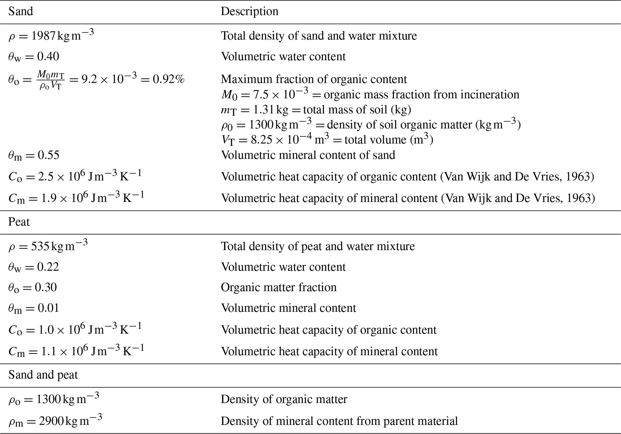
The agar gel was washed out using distilled water, and the cylindrical container was packed with soil. Two types of soil were used for the HPP tests: sand and peat. These soils are indicative of the physical extent of soil thermal properties. The soils were collected from field sites near Fort McMurray, Alberta. The sand contained small amounts of bitumen as representative of the Alberta Oil Sands area. Two independent laboratory analyses with incineration at 1100 ∘C were conducted on the sand, finding the total carbon content to range between a mean of 0.44 % and 0.75 % by mass. The soil properties are summarized in Table 1.
The water content for the sand was chosen so that the sand was saturated, whereas the water content for the peat was chosen so that the soil would remain as wet as possible (Table 1). Due to the absorbent characteristics of the peat soil, it was not possible during the time of the laboratory experiment to completely saturate the pore spaces of the soil column. However, the volumetric water content θ for both soils was chosen to ensure adequate contact between the probe and the soil and also to reduce air gaps that can increase thermal contact resistance and decrease the accuracy of the measurement (Liu and Si, 2010). These air gaps can occur in drier soils with lower water contents. Since comparisons are required to be made between heat pulse probe and gravimetric measurements for testing the in situ calibration procedure described in this paper, the presence of air gaps represents an additional source of error that was controlled.
Table 2Heat pulse strengths, time of heating and cooling, and total time for each experiment conducted on sand and peat. The experiment identifier is an alphabetical letter that identifies the experiment set. “No.” indicates the total number of experiments conducted per set.

Since the soil dried out over the time of multiple experiments, some additional water was added between successive days to ensure that the volumetric water content θ was close to the target value. Between trials, the top of the container was covered with a cap to reduce evaporation of water from the soil. Changes in water content occurred over the time of the experiment due to evaporation since the cap did not create a hermetic seal between the top of the container and the soil column. Table 1 shows quantities used for the application of HPP forward and inverse models to peat and sand.
Experiment sampling durations, q heat inputs, and heat durations are summarized in Table 2. Trial numbers of each experiment refer to groups of experiments conducted temporally close together.
The heat pulse strength and time of heating were chosen to minimize interaction of the heat pulse with the container boundaries. Due to the short time span over which each experiment was conducted in a laboratory setting, explicit correction was not applied for changes in ambient temperature (Young et al., 2008; Zhang et al., 2014). Between each experiment, the temperature of the soil column returned to a level that approximated the initial temperature before the probe was heated again for the next trial. All experiments were conducted at room temperature (∼ 20 ∘C).
Numerical comparisons were made using the root mean squared difference (RMSD) and mean bias (MB). The RMSD indicates the overall differences between two datasets. The MB indicates whether the model underpredicts or overpredicts relative to the observations.
3.1 Synthetic experiments
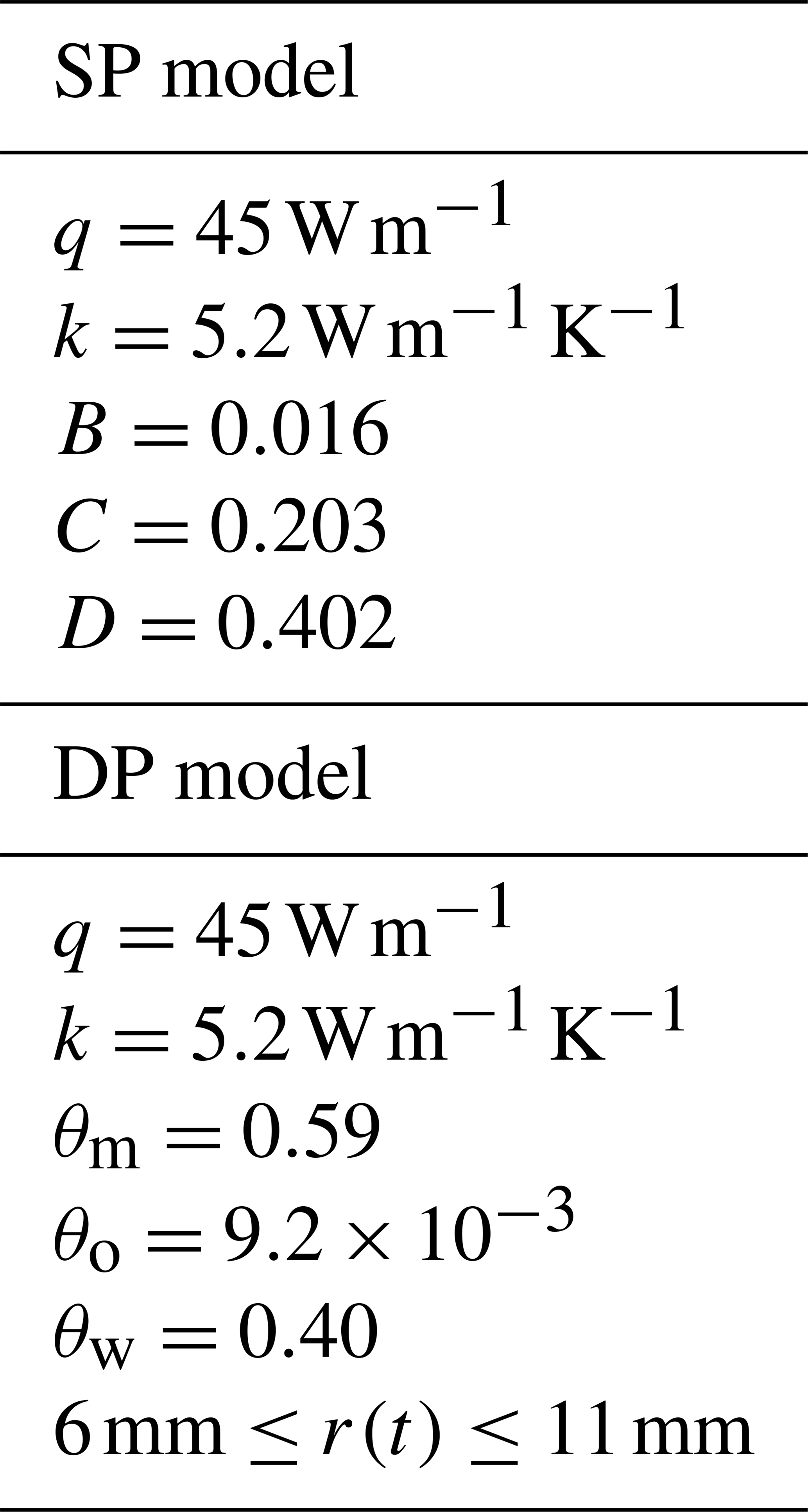
Synthetic heating curves were constructed using Eqs. (1) and (2) to serve as a forward model and provide a test of the signal processing. The SP and DP curves are shown as Figs. 3 and 4 and were generated using the model inputs given in Table 3. For the DP, the assumed change in probe spacing radius is shown for a linear increase (Fig. 4b), decrease (Fig. 4e), and Brownian random-walk-scaled so that the numerical values are between a starting and ending radius (Fig. 4h).
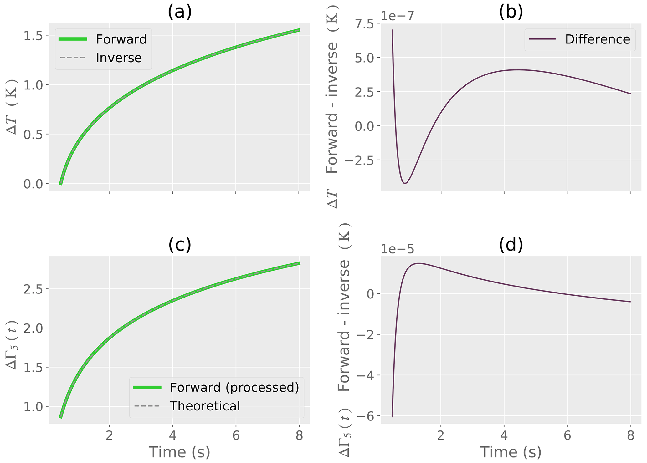
Figure 3Synthetic example of SP signal processing. (a) Forward model and reconstruction of the forward model by the inverse model. (b) Numerical difference between the forward and inverse models. (c) Forward model ΔΓ5(t) from the signal processing compared to the theoretical model of ΔΓ5(t). (d) Numerical difference between the forward model ΔΓ5(t) and the theoretical model.
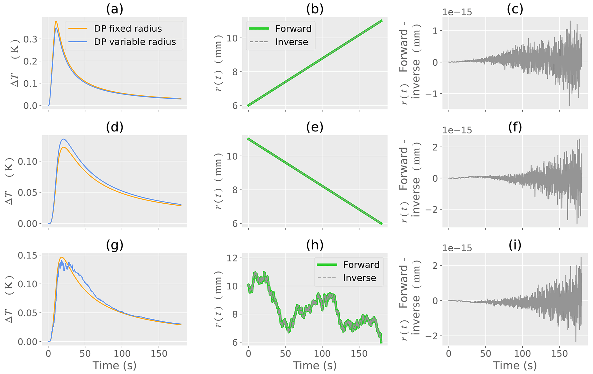
Figure 4Synthetic example of DP forward and inverse models. (a, d, g) DP temperature change ΔT with a fixed and variable radius. (b, e, h) Known change in r(t) as a variable radius. The forward and inverse model (reconstruction by signal processing) is shown. (c, f, i) Numerical difference between the forward and inverse models. Each row of Fig. 4 corresponds to a numerical experiment with an associated change in r(t) given in the second column (b, e, h).
The time-variable radius is r(t), and the associated curve is shown on the plots as a DP variable radius. The DP fixed radius curve is calculated using the first element of the r(t) used for a particular DP variable radius curve. The fixed radius is taken to be constant over the time of heating and cooling.
For the SP, Fig. 3a shows the forward model and the reconstruction of the forward model by the inverse model proposed in Sect. 2.2.1. The numerical difference between the forward and inverse models is shown by Fig. 3b and is on the order of . This difference occurs due to discretization of the numerical derivatives and floating-point round-off error from the homodyning process. The simplified model given by ΔΓ5(t) is shown by Fig. 3c and demonstrates the reduction of terms from the original model (Eq. 1). Figure 3d is the numerical difference between the forward and inverse models associated with ΔΓ5(t). The numerical difference remains small over the time of heating.

Figure 5Example signal processing for sand showing (a) the measured and modelled SP heating curves; (b) the measured and modelled DP heating curves along with the detected peak time; (c) the detected change in effective radius r(t) from the signal processing. The effective radius r(t) as obtained from signal processing compensates for model error, experimental error, and physical changes in the spacing of the heater needles.
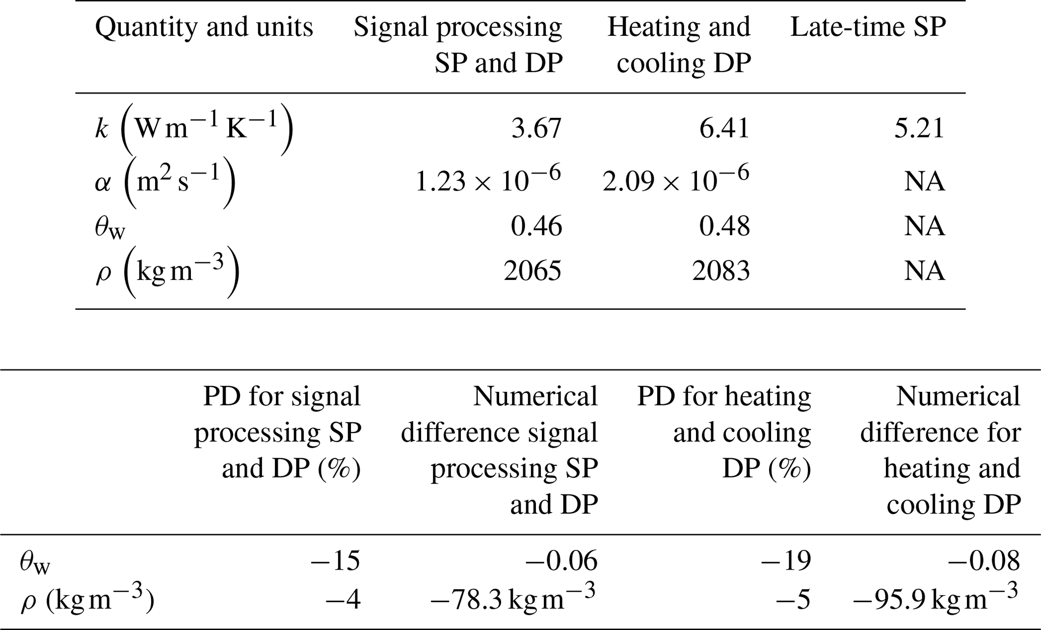
Figure 4 demonstrates the heating and cooling curves for a DP model with fixed radius and variable radius. The assumed time-variable radius r(t) is given along with the application of the inverse model proposed in Sect. 2.2.2. The first row of Fig. 4 (a–c) is for a linear increase; the second row of Fig. 4 (d–f) is for a linear decrease; and the third row of Fig. 4 (g–i) is for the Brownian random walk. The difference between the forward and inverse models is on the order of for all changes in probe spacing radius (Fig. 4c–i), indicating that for a synthetic model the error is mostly associated with floating-point calculations and that the inverse model is accurate.
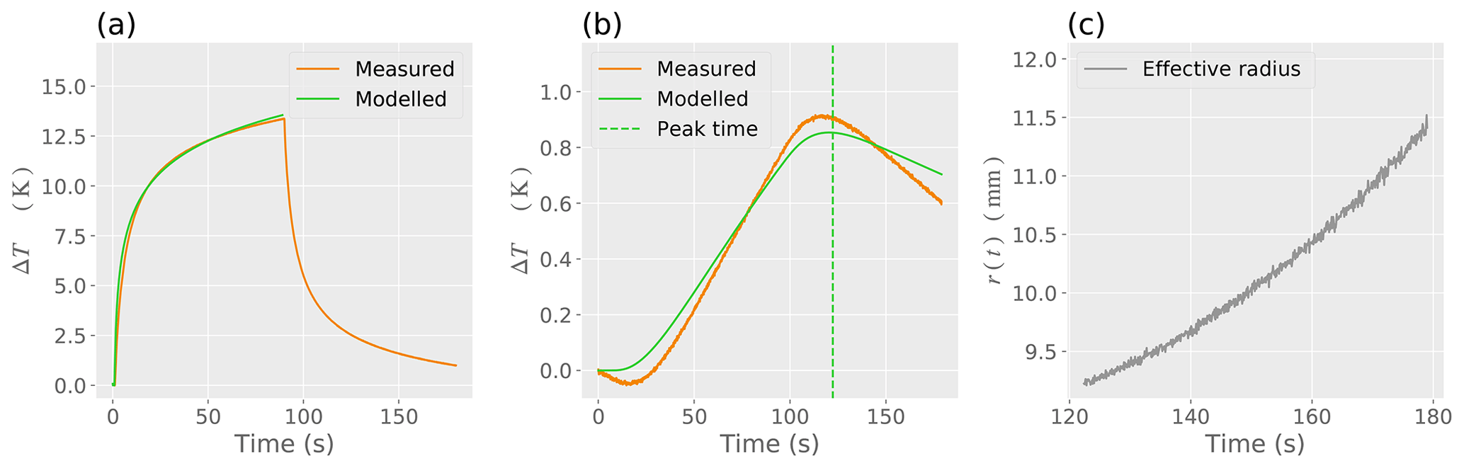
Figure 6Example signal processing for peat showing (a) the measured and modelled SP heating curves; (b) the measured and modelled DP heating curves along with the detected peak time; and (c) the detected change in effective radius r(t)from the signal processing. The effective radius r(t) as obtained from signal processing compensates for model error, experimental error, and physical changes in the spacing of the heater needles.
3.2 Soil data
Since the signal processing SP and signal processing DP models are applied together, hereafter these will be referred to as the signal processing SP and DP model. The late-time SP model is described in Sect. 2.2.1. The heating and cooling DP model refers to the nominal curve fitting using Eq. (2).
Figure 5 provides an example of the models applied to sand (Table 4). The peak time corresponding to tp+ta is indicated as a vertical line in Fig. 5b. Changes in effective radius r(t) determined by signal processing are shown as Fig. 5c. The rapid fluctuations in the effective radius r(t) occur due to temperature drift, model error, and experimental error. The signal processing thereby compensates for these effects using r(t) as an effective radius. Table 4 shows that the quantities found using all models have the same orders of magnitude and indicates that the signal processing SP and DP model is more accurate than the heating and cooling DP model compared to the gravimetric values used for the laboratory experiment.
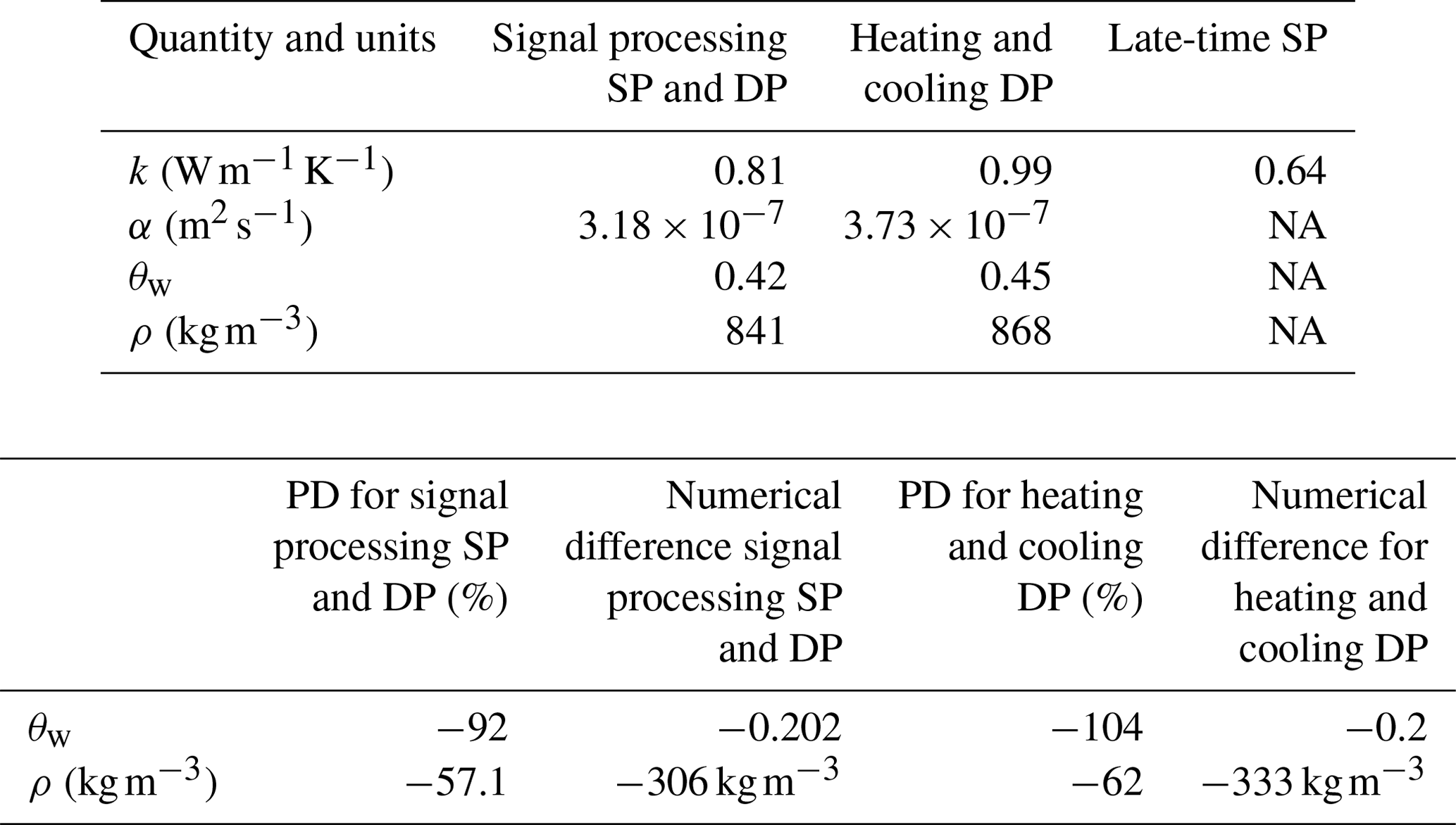
Figure 6 shows the signal processing SP and DP model applied to peat (Table 5). Compared to the sand example given above, the thermal conductivity k and diffusivity α are lower for the peat, demonstrating that the peat takes longer to warm up during the time of experiment. The heating and cooling curves are thereby distinctively different between sand and peat. However, in the same manner as the sand example, the quantities found using all models are of similar orders of magnitude. Figure 6c shows that there are fewer rapid fluctuations in the effective radius r(t) determined for peat compared to sand. Moreover, the change in effective radius is less pronounced for peat compared to sand due to smaller temperature drift associated with lower k and α. Also, in a similar fashion to sand, the percentage difference (PD) and numerical difference demonstrate that the signal processing models introduced in this paper are more accurate than the nominal models.
Figure 7 shows the thermal conductivity k and diffusivity α for the sand and peat determined for the experimental trials. For the sand, the nominal heating and cooling DP model provides estimates of k that are mostly higher than the signal processing SP and late-time SP models. The late-time SP model provides estimates of k that are intermediate between the other two models. The signal processing SP model produces the lowest estimates of k. However, the estimates of k made by all three models are the same orders of magnitude and remain relatively constant over experiments conducted on each soil type. The thermal diffusivity estimates provided by the heating and cooling DP model are slightly higher than the estimates provided by the signal processing SP and DP model for sand (Fig. 7c), whereas for peat (Fig. 7d) the thermal diffusivity for both models is approximately similar.
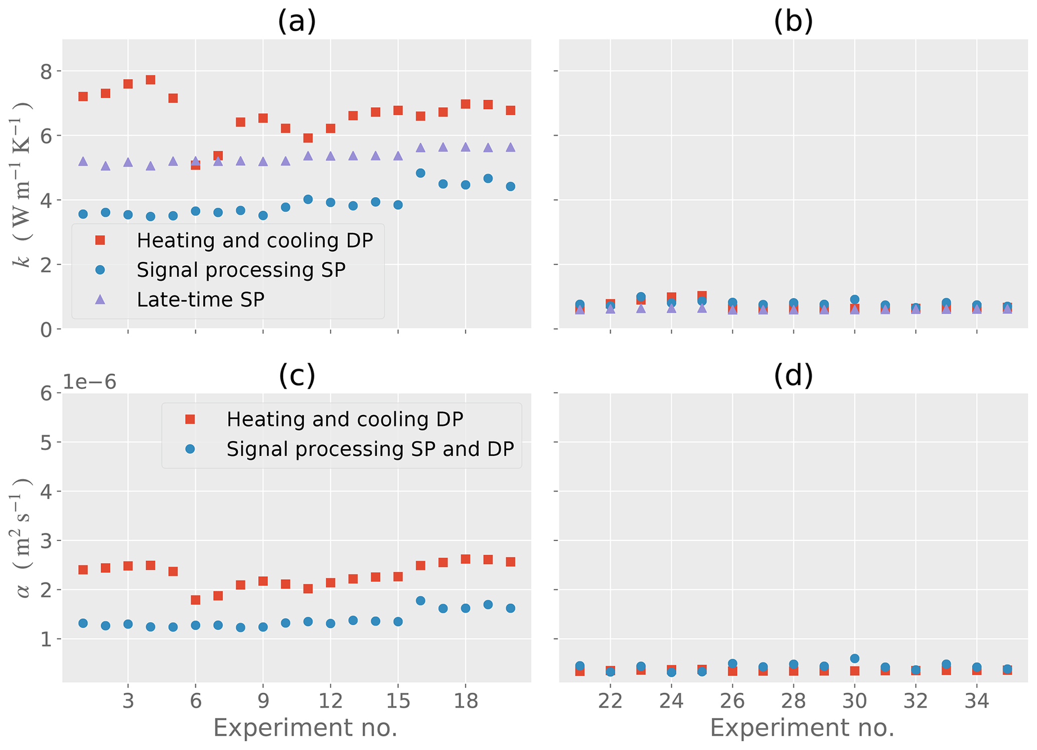
Figure 7Thermal conductivity k and thermal diffusivity α for each of the experiments. (a) Thermal conductivity for sand. (b) Thermal conductivity for peat. (c) Thermal diffusivity for sand. (d) Thermal diffusivity for peat.
Results corresponding to Figs. 7 an 8 are shown by Tables 6 and 7. These tables show the RMSD, MB, and PD, and the results of these calculations are discussed below.
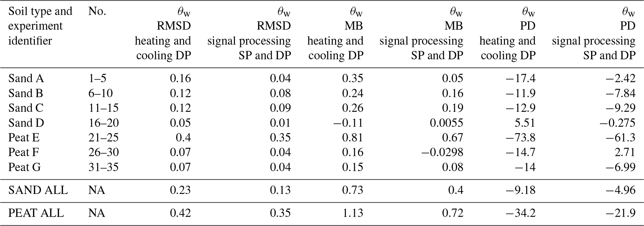
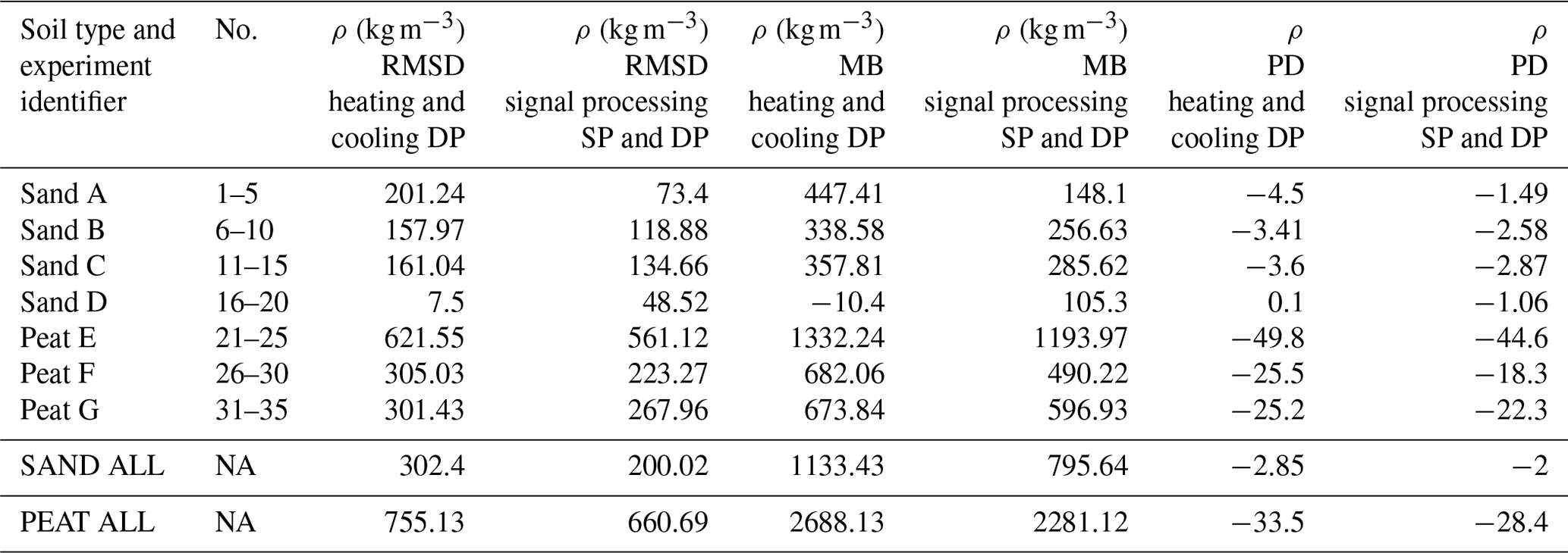
Figure 8 shows the determined values of water content θw and density ρ. Overall, for the sand and peat experiments, the nominal heating and cooling DP model has a higher-magnitude RMSD, MB, and PD compared to the signal processing SP and DP model introduced in this paper, indicating that the determination of the effective r(t) by signal processing improves estimates of θw and ρ.

Figure 8Water content θw and density ρ for each of the experiments. (a) Water content for sand. (b) Water content for peat. (c) Density for sand. (d) Density for peat.
For all sand experiments, the signal processing SP and DP model reduces the θw RMSD by 0.10 (10 %), the MB by 0.33 (33 %), and the PD by 4.2 % compared to the nominal heating and cooling DP model. For all peat experiments, the corresponding reduction for θw is 0.07 (7 %) for the RMSD, 0.41 (41 %) for the MB, and 12.3 % for the PD.
For the density ρ of sand, the signal processing SP and DP model reduces the RMSD by 102 kg m−3, the MB by 338 kg m−3, and the PD by 0.85 %. For the density ρ of peat, the signal processing SP and DP model reduces the RMSD by 94 kg m−3, the MB by 407 kg m−3, and the PD by 5.1 %.
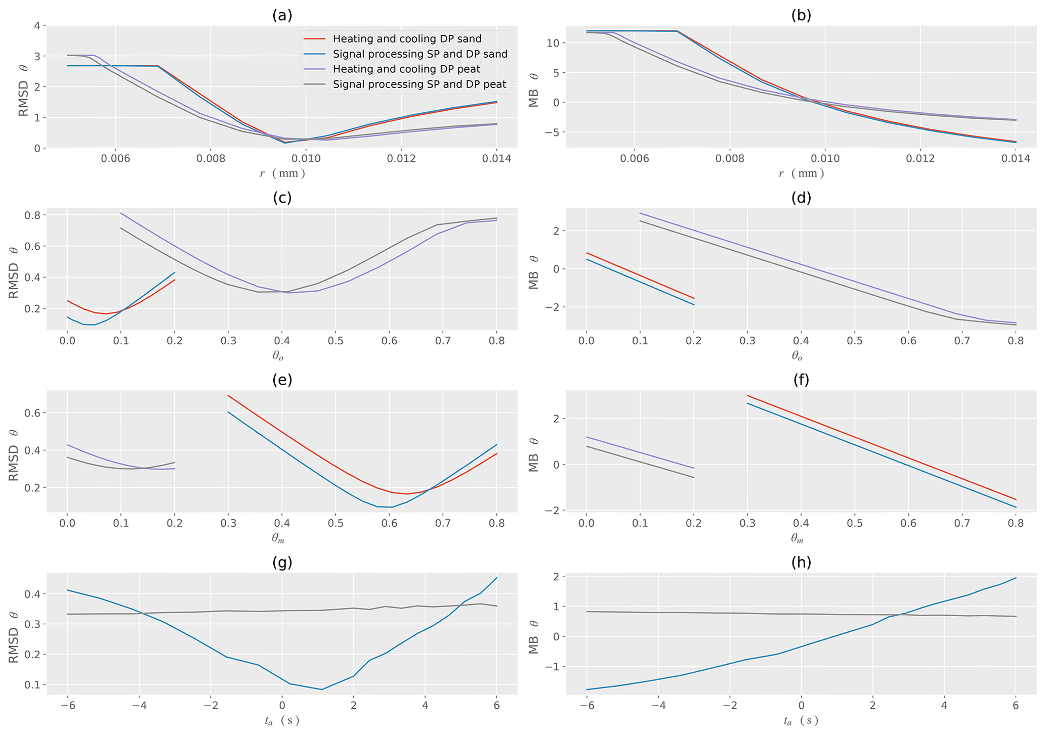
Figure 9Sensitivity analysis for water content θw for sand and peat with respect to the different models. (a) RMSD for changes in the calibrated initial radius r. (b) MB for changes in the calibrated initial radius. (c) RMSD for changes in the organic volume fraction θo. (d) MB for changes in the organic volume fraction θo. (e) RMSD for changes in the mineral volume fraction θm. (f) MB for changes in the mineral volume fraction θm. (g) RMSD for changes in the time delay ta. (h) MB for changes in the time delay ta.
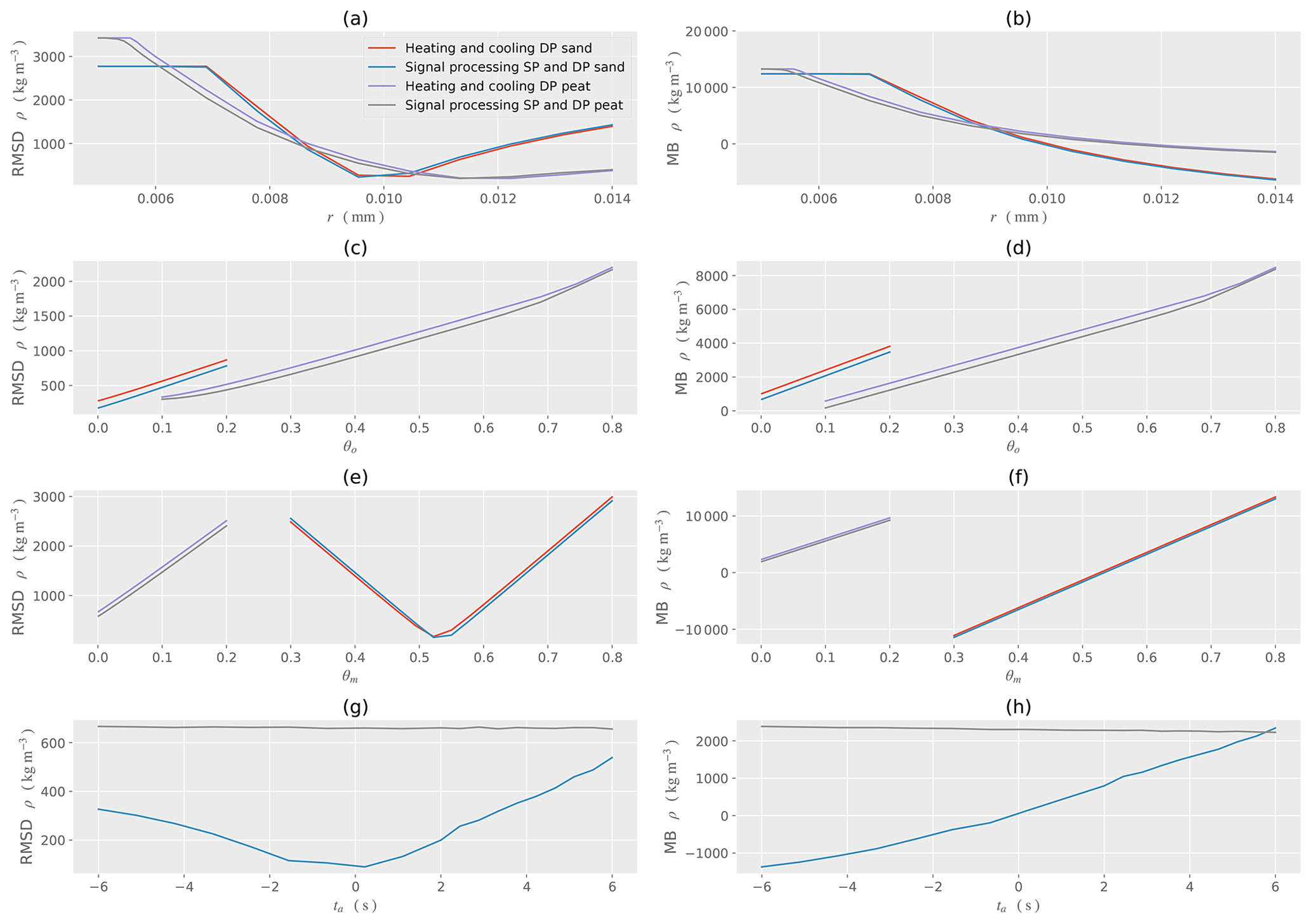
Figure 10Sensitivity analysis for density ρ for sand and peat with respect to the different models. (a) RMSD for changes in the calibrated initial radius r. (b) MB for changes in the calibrated initial radius. (c) RMSD for changes in the organic volume fraction θo. (d) MB for changes in the organic volume fraction θo. (e) RMSD for changes in the mineral volume fraction θm. (f) MB for changes in the mineral volume fraction θm. (g) RMSD for changes in the time delay ta. (h) MB for changes in the time delay ta.
For experiment identifiers A, B, C, and D associated with sand, the RMSD, MB, and PD magnitudes are lowest for θw determined from the signal processing SP and DP model compared to the nominal heating and cooling DP model. The RMSD, MB, and PD magnitudes are also lower for most sand estimates of ρ other than experiment identifier D, for which the RMSD and MB magnitudes are larger than magnitudes associated with the nominal heating and cooling DP model. The heat pulse strength and duration were of greater magnitude for experiment identifier D, but since ρ is being calculated as a function of θw this indicates a change in soil constituents (see Eq. 19) in the vicinity of the probe for experiment identifier D and demonstrates sensitivity of the signal processing to this change.
An increase in water content is apparent for experiment identifiers E to G associated with peat. The increase in water content occurred since the HPP experiments were initially conducted less than an hour after water was added to the soil column. Since the soil column was opaque, the infiltration of water in the column and the associated wetting front could not be tracked, and thereby localized volumes of water surrounding the HPP caused a rise in water content. Since the rise is consistent and shown by the heating and cooling DP model as well as the signal processing SP and DP model for θw and ρ (Fig. 8b and d), this indicates that both models are in physical agreement. Lower RMSD, MB, and PD values for the signal processing SP and DP model indicates that the signal processing introduced in this paper also improves estimates of θw and ρ when the water content changes during the time interval of experiment identifier E.
For experiment identifiers F and G, the determined θw and ρ remain approximately constant over time for peat. Compared to experiment identifier E, a reduction in water content has occurred due to infiltration over time and some loss of water due to evaporation. For these experiments, the RMSD, MB, and PD are lower for the signal processing SP and DP model compared to the heating and cooling DP model.
3.3 Sensitivity analysis
To identify the effects of model parameters on the RMSD and MB of model outputs θw and ρ, a sensitivity analysis (Figs. 9 and 10) was conducted over all data collected. The sensitivity analysis utilized the OAT (one-at-a-time) approach, whereby one variable at a time is changed, whereas the other model inputs are held constant (Hamby, 1994). Overall, for a range of nominal model inputs, Figs. 9 and 10 demonstrate that the signal processing associated with the signal processing SD and DP model reduces the RMSD and MB compared to the nominal heating and cooling DP model. This also indicates that the signal processing method produces more accurate estimates than the curve-fitting models nominally used for heat pulse probe experiments.
For all models and soils used to determine θw and ρ, the RMSD and MB are lowest when the initial radius rinitial is close to the calibrated value, indicating the importance of calibration for all models. If the rinitial is underpredicted, the MB indicates an overprediction of θw and ρ, whereas an overprediction of r0 indicates an underprediction of θw and ρ.
For sand θw, an organic content θo<0.1 produces the lowest-magnitude RMSD and MB, whereas for peat θw, an organic content close to θo≈0.40 produces the lowest-magnitude RMSD and MB. This physically approximates the composition of the sand and peat soils used for these experiments. The MB for sand and peat indicates a model overprediction for θo values lower than these thresholds and a model underprediction for θo values higher than these thresholds. A similar effect is also shown for the mineral content θm, with θm≈0.60 resulting in the lowest-magnitude RMSD and MB for sand. For peat, θm≈0.15 results in the lowest-magnitude RMSD and MB.
For sand θw the time delay ta≈1.5 s is a good assumption to provide the lowest values of RMSD and MB for the signal processing SD and DP model for both sand and peat. For peat ρ the time delay is ta≈0 s. The time delay ta is not a parameter for the nominal heating and cooling DP model, and a sensitivity analysis is not conducted for ta when using this model. Applied to peat, the signal processing SD and DP model is relatively insensitive to the time delay ta due to the lower thermal conductivity k and diffusivity α relative to sand that dampens changes in the effective radius r(t) as determined by signal processing.
In the context of the sensitivity analysis, as θo increases for sand, the RMSD and MB related to ρ also increase. For peat, a concomitant increase in θo is associated with an increase in the RMSD and MB, indicating that for ρ it is not possible to calibrate for θo and an approximation of θo must be known for model application within the context of these experiments. A mineral content of θm≈0.55 for sand produces the lowest RMSD and MB related to ρ. As θm increases for peat, the RMSD and MB also increase, indicating that for ρ it is once again not possible to calibrate for θm and an approximation must be utilized.
-
A novel circuit was designed and tested using a hybrid SP and DP heat pulse probe (HPP) design. The circuit utilized a PID controller to precisely control the heat input into the soil. In lieu of a variable resistor, this enabled the heat input q to be changed by a computer or a datalogger. When deployed at a remote or inaccessible field site, the HPP heat input can be set to a given value using the communication interfaces. This enables the heat input to be appropriately selected for soil type.
-
Instead of using a 1 Ω sense resistor to infer heat inputs into the soil, the circuit used a resistor with a 0.01 Ω nominal resistance. This reduced the voltage drop across the sense resistor and still allowed the current through the nichrome wire to be adequately determined during the time of experiment, although a differential amplifier was required to detect the voltage difference before digitization by an ADC.
-
A sampling rate of 120 Hz was required for application of the PID controller and theory associated with signal processing related to a hybrid SP and DP heat pulse probe. The higher sampling rate allowed digital filtering to be applied.
-
Signal processing was used to determine thermal conductivity using an SP model that did not rely on a late-time SP approximation. A DP model was used to determine changes in the effective DP probe spacing radius.
-
The DP and SP signal processing models introduced in this paper improved overall estimates of soil water content θw and bulk soil density ρ for sand and peat soils, indicating that the detection of effective changes in the probe spacing radius using signal processing is useful to correct for model error and physical changes in the probe spacing. This improvement is associated with standard HP and DP probes that are used together in a novel fashion along with signal processing.
-
Further research is required to test the signal processing models introduced in this paper and to compare the estimates of soil water content θw and bulk soil density ρ to estimates made using other measurement systems and technologies. The effective radius calibration has an advantage for soil types wherein expansion and contraction of the soil can cause changes in the effective probe spacing radius r(t).
To efficiently obtain the inverse of Ei(x), endpoints for a search interval need to be appropriately selected, particularly when the inverse model runs on an embedded resource-constrained microcontroller. To ensure numerical continuity and accuracy between the forward and inverse models, the same Ei(x) function is used in the inverse of Ei(x) in lieu of alternative numerical approximations.
Take , where E1(x)=En(x) with n=1. Let x>0 and we need to show
Using 5.1.20 of Abramowitz and Stegun (1964), we need to show that with x>0
Since and as x→∞, then as x→∞. Therefore, . We next show
Algebraic rearrangement yields
Since x>0, we need to show
By algebraic rearrangement, we find
The right-hand side can be replaced by a power series representation:
The proof proceeds by contradiction and shows that the inequality holds. We assume
However, this is a contradiction, so inequality Eq. (A1) holds.
From inequality Eq. (A1), the search interval for Ei(x) is for x<0. The inverse of Ei(x) is computed using Golden-section search (Kiefer, 1953) on the bounded interval.
The following shows how endpoints of the search interval for the inverse are selected for the cooling section of the DP curve using the result given above. Without the q∕(4πk) term, Eq. (4) is of the form
Let and , where and x>0 and y>0. Equation (A2) can be rewritten as
From the above and inequality (A1),
Algebraic manipulation yields the following search interval for t>th:
Golden-section search with the inequality Eq. (A3) can cause numerical underflow when computing f(h) near the right endpoint of the search interval. In lieu of Golden-section search, the inverse for the cooling section is computed using Nelder–Mead optimization with the inequality Eq. (A3) used as a Box constraint (Box, 1965).
| Acronyms | |
|---|---|
| ADC | Analog-to-digital converter |
| AFE | Analog front end |
| COTS | Commercial off-the-shelf |
| DAC | Digital-to-analog converter |
| DC | Direct current |
| DP | Dual probe |
| HPP | Heat pulse probe |
| MB | Mean bias |
| M2M | Machine-to-machine |
| NA | Not applicable |
| OAT | One-at-a-time |
| PCB | Printed circuit board |
| PD | Percentage difference |
| PID | Proportional–integral–derivative controller |
| PLL | Phase-locked loop |
| PVC | Polyvinyl chloride |
| RMSD | Root mean squared difference |
| RS-232 | Recommended standard 232 serial port |
| SDI-12 | Serial digital interface at 1200 baud |
| SDRAM | Synchronous dynamic random-access memory |
| SP | Single probe |
| USB | Universal serial bus |
| Symbols and SI units | |
|---|---|
| ai | log (r(ti)) |
| α | Thermal diffusivity of soil (m2 s−1) |
| Coefficients used for the SP model | |
| Ch | Volumetric heat capacity () |
| Volumetric heat capacity (mineral, organic, and water) | |
| c | Specific heat capacity () |
| {cm,co} | Specific heat capacity (mineral, organic) () |
| ΔΓ(t) | Change in temperature (K) as a function of time for SP |
| γ(r,t) or γ(r(t),t) | Signal processing computation step |
| d∕dt | Time derivative |
| ΔE | Voltage drop over resistive element (V) |
| Ei(x) | Exponential integral function |
| Ekn | Known (measured) output voltage (V) |
| f(x,y) | Function of x,y |
| fs | Sampling rate (Hz) |
| H | r2∕4α |
| Volume fractions (mineral, organic, and water) | |
| I | Current through nichrome heater wire (A) |
| i | Integer index |
| k | Thermal conductivity () |
| ℓ | Length of heater needle (m) |
| log ( ) | Natural logarithm function |
| N | Index number as integer |
| π | ≈3.14159 |
| P | Electrical power (W) |
| ρ | Density (kg m−3) |
| {ρm,ρo} | Densities (mineral, organic) (kg m−3) |
| q | Energy transfer per time per length of heater needle (W m−1) |
| Rs | Resistance of sensor resistor (Ω) |
| Rw | Resistance of nichrome heater wire (Ω) |
| r(t) | Effective DP radius as a function of time (m) |
| r | DP radius (m) |
| rinitial | Initial DP radius (m) |
| rn | Radius of heater needle (m) |
| t | Time (s) |
| t0 | Start time of heating nichrome wire (s) |
| ta | Additional time delay (s) |
| tc | Time of cooling (s) |
| td | Time at which curve is assumed to be linear (s) |
| th | Stop time of heating nichrome wire (s) |
| ti | Time used to determine initial temperature (s) |
| tp | Time at which curve is at a maximum peak (s) |
| Total time of experiment (s) | |
| ΔT(t) | Change in temperature (K) as a function of time for DP |
| As the time step (s) | |
| Real numbers | |
| || | Absolute value function |
The computer code and data used to produce the figures and numerical results in this paper can be downloaded from Figshare (https://doi.org/10.6084/m9.figshare.11372181, Kinar, 2020).
The data from the experiments described in this paper can also be obtained from the Figshare data repository as a separate download (https://doi.org/10.6084/m9.figshare.11371455, Kinar, 2019).
NJK, BS, and JWP were responsible for conceptualization. NJK and BS designed the methodology. NJK developed the software. NJK and BS performed validation. NJK conducted the formal analysis. NJK and BS carried out the investigation. BS and JWP acquired resources. NJK was responsible for data curation. NJK prepared the original draft; NJK, JWP, and BCS were responsible for review and editing. NJK prepared the visualization. NJK, BS, and JWP provided supervision. NJK, JWP, and BS were responsible for project administration. JWP and BS were responsible for funding acquisition.
The authors declare that they have no conflict of interest.
Eric Neil (Department of Soil Science, College of Agriculture and Bioresources, University of Saskatchewan) is thanked for assistance with the setup and execution of the laboratory experiments detailed in this paper. We would like to acknowledge funding from the Canada First Research Excellence Fund's Global Water Futures Program, the Natural Sciences and Engineering Research Council of Canada, the Canada Research Chairs Program, and the Canadian Department of Western Economic Diversification (WED). We thank two anonymous reviewers and one identified reviewer (Stephen Drake) for insightful comments that have greatly improved this paper.
This research has been supported by the Canada First Research Excellence Fund's Global Water Futures Program, the Natural Sciences and Engineering Research Council of Canada, the Canada Research Chairs Program, and the Canadian Department of Western Economic Diversification (WED).
This paper was edited by Lev Eppelbaum and reviewed by Stephen Drake and two anonymous referees.
Abramowitz, M. and Stegun, I. A.: Handbook of mathematical functions with formulas, graphs, and mathematical tables, Courier Dover Publications, New York, USA, 1964.
Abu-Hamdeh, N. H.: Measurement of the thermal conductivity of sandy loam and clay loam soils using single and dual probes, J. Agr. Eng. Res., 80, 209–216, https://doi.org/10.1006/jaer.2001.0730, 2001.
Abu-Hamdeh, N. H. and Reeder, R. C.: Soil thermal conductivity: effects of density, moisture, salt concentration, and organic matter, Soil Sci. Soc. Am. J., 64, 1285, https://doi.org/10.2136/sssaj2000.6441285x, 2000.
Ang, K. H., Chong, G., and Li, Y.: PID control system analysis, design, and technology, IEEE T. Cont. Syst. T., 13, 559–576, https://doi.org/10.1109/TCST.2005.847331, 2005.
Basinger, J. M., Kluitenberg, G. J., Ham, J. M., Frank, J. M., Barnes, P. L., and Kirkham, M. B.: Laboratory evaluation of the dual-probe heat-pulse method for measuring soil water content, Vadose Zone J., 2, 389–399, https://doi.org/10.2113/2.3.389, 2003.
Blackwell, J. H.: A transient-flow method for determination of thermal constants of insulating material in bulk, J. Appl. Phys., 25, 137–144, 1954.
Box, M. J.: A new method of constrained optimization and a comparison with other methods, Comput. J., 8, 42–52, https://doi.org/10.1093/comjnl/8.1.42, 1965.
Bristow, K. L.: Measurement of thermal properties and water content of unsaturated sandy soil using dual-probe heat-pulse probes, Agr. Forest Meteorol., 89, 75–84, https://doi.org/10.1016/S0168-1923(97)00065-8, 1998.
Bristow, K. L., Campbell, G. S., and Calissendorff, K.: Test of a Heat-Pulse Probe for Measuring Changes in Soil Water Content, Soil Sci. Soc. Am. J., 57, 930–934, https://doi.org/10.2136/sssaj1993.03615995005700040008x, 1993.
Bristow, K. L., White, R. D., and Kluitenberg, G. J.: Comparison of single and dual probes for measuring soil thermal properties with transient heating, Aust. J. Soil Res., 32, 447–464, https://doi.org/10.1071/SR9940447, 1994.
Bristow, K. L., Kluitenberg, G. J., Goding, C. J., and Fitzgerald, T. S.: A small multi-needle probe for measuring soil thermal properties, water content and electrical conductivity, Comput. Electron. Agr., 31, 265–280, https://doi.org/10.1016/S0168-1699(00)00186-1, 2001.
Campbell, G. S., Calissendorff, C., and Williams, J. H.: Probe for measuring soil specific heat using a heat-pulse method, Soil Sci. Soc. Am. J., 55, 291–293, 1991.
Carter, B. C., Vershinin, M., and Gross, S. P.: A comparison of step-detection methods: how well can you do?, Biophys. J., 94, 306–319, https://doi.org/10.1529/biophysj.107.110601, 2008.
De Vries, D. A.: A nonstationary method for determining thermal conductivity of soil in situ, Soil Sci., 73, 83–89, 1952.
Dias, P. C., Roque, W., Ferreira, E. C., and Siqueira Dias, J. A.: A high sensitivity single-probe heat pulse soil moisture sensor based on a single NPN junction transistor, Comput. Electron. Agr., 96, 139–147, https://doi.org/10.1016/j.compag.2013.05.003, 2013.
Ebdon, D.: Statistics in Geography: a practical approach – revised with 17 programs, 2nd edn., Wiley-Blackwell, Oxford, UK, New York, USA, 1991.
Green, S., Clothier, B., and Jardine, B.: Theory and Practical Application of Heat Pulse to Measure Sap Flow, Agron. J., 95, 1371, https://doi.org/10.2134/agronj2003.1371, 2003.
Ham, J. M. and Benson, E. J.: On the construction and calibration of dual-probe heat capcity sensors, Soil Sci. Soc. Am. J., 68, 1185–1190, 2004.
Hamby, D. M.: A review of techniques for parameter sensitivity analysis of environmental models, Environ. Monit. Assess., 32, 135–154, https://doi.org/10.1007/BF00547132, 1994.
Hamming, R. W.: Digital Filters, 2nd edn., Prentice-Hall, Englewood Cliffs, NJ, 1983.
He, H., Dyck, M. F., Horton, R., Ren, T., Bristow, K. L., Lv, J., and Si, B.: Development and Application of the Heat Pulse Method for Soil Physical Measurements, Rev. Geophys., 56, 567–620, https://doi.org/10.1029/2017RG000584, 2018.
Heitman, J. L., Basinger, J. M., Kluitenberg, G. J., Ham, J. M., Frank, J. M., and Barnes, P. L.: Field evaluation of the dual-probe heat-pulse method for measuring soil water content, Vadose Zone J., 2, 552–560, https://doi.org/10.2113/2.4.552, 2003.
Hopmans, J. W., Šimunek, J., and Bristow, K. L.: Indirect estimation of soil thermal properties and water flux using heat pulse probe measurements: Geometry and dispersion effects, Water Resour. Res., 38, 7-1-7–14, https://doi.org/10.1029/2000WR000071, 2002.
Jin, H., Wang, Y., Zheng, Q., Liu, H., and Chadwick, E.: Experimental study and modelling of the thermal conductivity of sandy soils of different porosities and water contents, Appl. Sci.-Basel, 7, 119, https://doi.org/10.3390/app7020119, 2017.
Kamai, T., Tuli, A., Kluitenberg, G. J., and Hopmans, J. W.: Soil water flux density measurements near 1 cm/d using an improved heat pulse probe design, Water Resour. Res., 44, W00D14, https://doi.org/10.1029/2008WR007036, 2008.
Kiefer, J.: Sequential Minimax Search for a Maximum, P. Am. Math. Soc., 4, 502–506, https://doi.org/10.2307/2032161, 1953.
Kinar, N. J. and Pomeroy, J. W.: Measurement of the physical properties of the snowpack, Rev. Geophys., 53, 481–544, https://doi.org/10.1002/2015RG000481, 2015.
Kinar, N.: Model code and software from paper: Signal Processing for In-Situ Detection of Effective Heat Pulse Probe Spacing Radius as the Basis of a Self-Calibrating Heat Pulse Probe, code available at: https://doi.org/10.6084/m9.figshare.11372181 (last access: 14 July 2020), 2020.
Kinar, N.: Dataset from paper: Signal Processing for In-Situ Detection of Effective Heat Pulse Probe Spacing Radius as the Basis of a Self-Calibrating Heat Pulse Probe, Dataset, https://doi.org/10.6084/m9.figshare.11371455 (last access: 14 July 2020), 2019.
Kluitenberg, G. J.: Heat Capacity and Specific Heat, in: Methods of Soil Analysis: Part 4 – Physical Methods, edited by: Dane, J. H. and Topp, C. G., Soil Science Society of America, Wisconsin, USA, 1201–1208, 2002.
Kluitenberg, G. J., Ham, J. M., and Bristow, K. L.: Error analysis of the heat pulse method for measuring soil volumetric heat capacity, Soil Sci. Soc. Am. J., 57, 1444–1451, 1993.
Kluitenberg, G. J., Das, B. S., and Bristow, K. L.: Error analysis of heat pulse method for measuring soil heat capacity, diffusivity, and conductivity, Soil Sci. Soc. Am. J., 59, 719, https://doi.org/10.2136/sssaj1995.03615995005900030013x, 1995.
Kluitenberg, G. J., Kamai, T., Vrugt, J. A., and Hopmans, J. W.: Effect of probe deflection on dual-probe heat-pulse thermal conductivity measurements, Soil Sci. Soc. Am. J., 74, 1537, https://doi.org/10.2136/sssaj2010.0016N, 2010.
Li, M., Si, B. C., Hu, W., and Dyck, M.: Single-probe heat pulse method for soil water content determination: comparison of methods, Vadose Zone J., 15, 1–13, https://doi.org/10.2136/vzj2016.01.0004, 2016.
Liu, G. and Si, B. C.: Dual-probe heat pulse method for snow density and thermal properties measurement, Geophys. Res. Lett., 35, 1–5, https://doi.org/10.1029/2008GL034897, 2008.
Liu, G. and Si, B. C.: Errors analysis of heat pulse probe methods: experiments and simulations, Soil Sci. Soc. Am. J., 74, 797–803, 2010.
Liu, G. and Si, B.: Soil ice content measurement using a heat pulse probe method, Can. J. Soil Sci., 91, 235–246, https://doi.org/10.4141/cjss09120, 2011.
Liu, G., Li, B., Ren, T., and Horton, R.: Analytical solution of the heat pulse method in a parallelepiped sample space, Soil Sci. Soc. Am. J., 71, 1607–1619, 2007.
Liu, G., Wen, M., Chang, X., Ren, T., and Horton, R.: A self-calibrated dual probe heat pulse sensor for in situ calibrating the probe spacing, Soil Sci. Soc. Am. J., 77, 417, https://doi.org/10.2136/sssaj2012.0434n, 2013.
Liu, G., Wen, M., Ren, R., Si, B., Horton, R., and Hu, K.: A general in situ probe spacing correction method for dual probe heat pulse sensor, Agr. Forest Meteorol., 226–227, 50–56, https://doi.org/10.1016/j.agrformet.2016.05.011, 2016.
Miner, G. L., Ham, J. M., and Kluitenberg, G. J.: A heat-pulse method for measuring sap flow in corn and sunflower using 3D-printed sensor bodies and low-cost electronics, Agr. Forest Meteorol., 246, 86–97, https://doi.org/10.1016/j.agrformet.2017.06.012, 2017.
Mori, Y., Hopmans, J. W., Mortensen, A. P., and Kluitenberg, G. J.: Multi-functional heat pulse probe for the simultaneous measurement of soil water content, solute concentration, and heat transport parameters, Vadose Zone J., 2, 561–571, https://doi.org/10.2113/2.4.561, 2003.
Morin, S., Domine, F., Arnaud, L., and Picard, G.: In-situ monitoring of the time evolution of the effective thermal conductivity of snow, Cold Reg. Sci. Technol., 64, 73–80, https://doi.org/10.1016/j.coldregions.2010.02.008, 2010.
Ochsner, T. E. and Baker, J. M.: In situ monitoring of soil thermal properties and heat flux during freezing and thawing, Soil Sci. Soc. Am. J., 72, 1025, https://doi.org/10.2136/sssaj2007.0283, 2008.
Ochsner, T. E., Horton, R., and Ren, T.: A new perspective on soil thermal properties, Soil Sci. Soc. Am. J., 65, 1641–1647, https://doi.org/10.2136/sssaj2001.1641, 2001.
Oppenheim, A., Kopec, G., and Tribolet, J.: Signal analysis by homomorphic prediction, IEEE T. Acoust. Speech, 24, 327–332, https://doi.org/10.1109/TASSP.1976.1162828, 1976.
Pearsall, K. R., Williams, L. E., Castorani, S., Bleby, T. M., and McElrone, A. J.: Evaluating the potential of a novel dual heat-pulse sensor to measure volumetric water use in grapevines under a range of flow conditions, Funct. Plant Biol., 41, 874, https://doi.org/10.1071/FP13156, 2014.
Penner, E.: Thermal conductivity of frozen soils, Can. J. Earth Sci., 7, 982–987, https://doi.org/10.1139/e70-091, 1970.
Ramires, M. L. V., Nieto de Castro, C. A., Nagasaka, Y., Nagashima, A., Assael, M. J., and Wakeham, W. A.: Standard Reference Data for the Thermal Conductivity of Water, J. Phys. Chem. Ref. Data, 24, 1377, https://doi.org/10.1063/1.555963, 1995.
Ravazzani, G.: Open hardware portable dual-probe heat-pulse sensor for measuring soil thermal properties and water content, Comput. Electron. Agr., 133, 9–14, https://doi.org/10.1016/j.compag.2016.12.012, 2017.
Saito, H., Šimůnek, J., and Mohanty, B. P.: Numerical analysis of coupled water, vapor, and heat transport in the vadose zone, Vadose Zone J., 5, 784–800, https://doi.org/10.2136/vzj2006.0007, 2006.
Saito, H., Šimůnek, J., Hopmans, J. W., and Tuli, A.: Numerical evaluation of alternative heat pulse probe designs and analyses, Water Resour. Res., 43, W07408, https://doi.org/10.1029/2006WR005320, 2007.
Sherfy, A. C., Lee, J., Tyner, J. S., and Kim, Y.: Improved Calibration for Estimating Soil Properties with a Multifunctional Heat Pulse Probe, Commun. Soil Sci. Plan., 47, 305–312, https://doi.org/10.1080/00103624.2015.1123266, 2016.
Song, Y., Ham, J. M., Kirkham, M. B., and Kluitenberg, G. J.: Measuring soil water content under turfgrass using the dual-probe heat-pulse technique, Journal of the American Society for Horticultural Science, 123, 937–941, https://doi.org/10.21273/JASHS.123.5.937, 1998.
Steinhart, J. S. and Hart, S. R.: Calibration curves for thermistors, Deep Sea Research and Oceanographic Abstracts, 15, 497–503, https://doi.org/10.1016/0011-7471(68)90057-0, 1968.
Sturm, M. and Johnson, J. B.: Thermal conductivity measurements of depth hoar, J. Geophys. Res., 97, 2129–2139, 1992.
Trautz, A. C., Smits, K. M., Schulte, P., and Illangasekare, T. H.: Sensible heat balance and heat-pulse method applicability to in situ soil-water evaporation, Vadose Zone J., 13, 1–11, https://doi.org/10.2136/vzj2012.0215, 2014.
Valente, A., Morais, R., Tuli, A., Hopmans, J. W., and Kluitenberg, G. J.: Multi-functional probe for small-scale simultaneous measurements of soil thermal properties, water content, and electrical conductivity, Sensor. Actuat. A-Phys., 132, 70–77, https://doi.org/10.1016/j.sna.2006.05.010, 2006.
Van Wijk, W. R. and De Vries, D. A.: Periodic temperature variations in a homogeneous soil, in: Physics of Plant Environment, edited by: Van Wijk, W. R., North-Holland Publishing Company, Amsterdam, 102–143, 1963.
Wagner, W. and Pruß, A.: The IAPWS Formulation 1995 for the Thermodynamic Properties of Ordinary Water Substance for General and Scientific Use, J. Phys. Chem. Ref. Data, 31, 387–535, https://doi.org/10.1063/1.1461829, 2002.
Wang, Q., Ochsner, T. E., and Horton, R.: Mathematical analysis of heat pulse signals for soil water flux determination, Water Resour. Res., 38, 27–1, https://doi.org/10.1029/2001WR001089, 2002.
Wen, M., Liu, G., Li, B., Si, B. C., and Horton, R.: Evaluation of a self-correcting dual probe heat pulse sensor, Agr. Forest Meteorol., 200, 203–208, https://doi.org/10.1016/j.agrformet.2014.09.022, 2015.
Yang, C. and Jones, S. B.: INV-WATFLX, a code for simultaneous estimation of soil properties and planar vector water flux from fully or partly functioning needles of a penta-needle heat-pulse probe, Computers and Geosciences, 35, 2250–2258, https://doi.org/10.1016/j.cageo.2009.04.005, 2009.
Young, M. H., Campbell, G. S., and Yin, J.: Correcting dual-probe heat-pulse readings for changes in ambient temperature, Vadose Zone J., 7, 22–30, https://doi.org/10.2136/vzj2007.0015, 2008.
Yun, T. S. and Santamarina, J. C.: Fundamental study of thermal conduction in dry soils, Granul. Matter, 10, 197, https://doi.org/10.1007/s10035-007-0051-5, 2008.
Zhang, Y., Treberg, M., and Carey, S. K.: Evaluation of the heat pulse probe method for determining frozen soil moisture content, Water Resour. Res., 47, https://doi.org/10.1029/2010WR010085, 2011.
Zhang, X., Heitman, J., Horton, R., and Ren, T.: Measuring near-surface soil thermal properties with the heat-pulse method: correction of ambient temperature and soil–air interface effects, Soil Sci. Soc. Am. J., 78, 1575, https://doi.org/10.2136/sssaj2014.01.0014, 2014.