the Creative Commons Attribution 4.0 License.
the Creative Commons Attribution 4.0 License.
 | 18 Aug 2020
The 1958 Lituya Bay tsunami – pre-event bathymetry reconstruction and 3D numerical modelling utilising the computational fluid dynamics software Flow-3D
Andrea Franco
Jasper Moernaut
Barbara Schneider-Muntau
Michael Strasser
Bernhard Gems
This study aims to test the capacity of Flow-3D regarding the simulation of a rockslide-generated impulse wave by evaluating the influences of the extent of the computational domain, the grid resolution, and the corresponding computation times on the accuracy of modelling results. A detailed analysis of the Lituya Bay tsunami event (1958, Alaska, maximum recorded run-up of 524 m a.s.l.) is presented. A focus is put on the tsunami formation and run-up in the impact area. Several simulations with a simplified bay geometry are performed in order to test the concept of a “denser fluid”, compared to the seawater in the bay, for the impacting rockslide material. Further, topographic and bathymetric surfaces of the impact area are set up. The observed maximum run-up can be reproduced using a uniform grid resolution of 5 m, where the wave overtops the hill crest facing the slide source and then flows diagonally down the slope. The model is extended along the entire bay to simulate the wave propagation. The tsunami trimline is well recreated when using (a) a uniform mesh size of 20 m or (b) a non-uniform mesh size of 15 m × 15 m × 10 m with a relative roughness of 2 m for the topographic surface. The trimline mainly results from the primary wave, and in some locations it also results from reflected waves. The denser fluid is a suitable and simple concept to recreate a sliding mass impacting a waterbody, in this case with maximum impact speed of ∼93 m s−1. The tsunami event and the related trimline are well reproduced using the 3D modelling approach with the density evaluation model available in Flow-3D.


The analysis and management of the hydrological and geological risks in mountain regions are nowadays considered a priority for human and territorial safety. Obtaining an accurate understanding of phenomena like landslides, flash floods, and landslide-generated impulse waves has been and still is a major challenge for reliable natural hazards assessment. In recent decades, the awareness of natural hazard events such as tsunamis in lakes and artificial basins (known as impulse waves) has increased since several disasters occurred (e.g. Tafjord, Norway, in 1934, Holmsen, 1936; Furseth, 1958; Harbitz et al., 1993; Braathen et al., 2004; Lituya Bay, Alaska, USA, in 1958, Miller, 1960; Vajont, Italy, in 1963, Paronuzzi and Bolla, 2012; Chehalis lake, Canada, in 2007, Wang et al., 2015; Aysen Fjord, Chile, in 2007, Sepúlveda et al., 2010; Taan Fjord, Alaska, USA, in 2015, Haeussler et al., 2018; Karrat Fjord, Greenland, in 2017, Gauthier et al., 2017). Such tsunamis can be induced by both sub-aquatic and subaerial landslides (Basu et al., 2010). The construction of new reservoirs for hydroelectric power generation in steep mountain valleys has highlighted the importance of risk evaluation for this type of natural hazard, particularly in the case of the Vajont catastrophe (10 October 1963, Italy), where an enormous landslide collapsed into the reservoir and triggered one of the largest impulse waves ever recorded, killing ∼2000 individuals (Paronuzzi and Bolla, 2012).
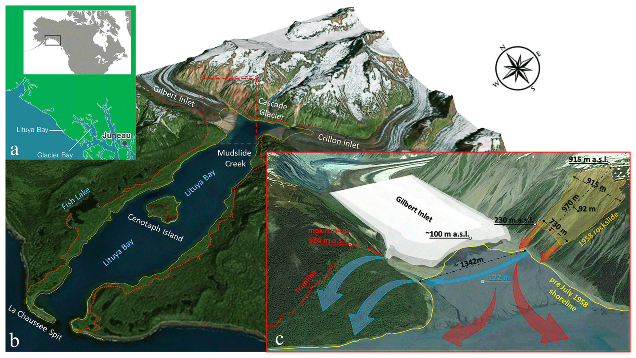
Figure 1(a) Location of Lituya Bay, in southeastern Alaska (modified from Bridge, 2018). (b) View of Lituya Bay: the yellow line represents the shoreline before July 1958, and the red line shows the trimline of the tsunami. (c) Gilbert Inlet, showing the situation in July 1958 pre- and post-tsunami: the rockslide dimension (orange), the maximum bay floor depth of −122 m (light blue), and the maximum run-up of 524 m a.s.l. (Miller, 1960) on the opposite slope with respect to the impact area are indicated (topography data from © Google Earth Pro 7.3.2.5776; last access: 24 April 2020).

Figure 2Rockslide source and opposite-facing slope of the maximum run-up (info according from the interpretation of Ward and Day, 2010; see Fig. 1). (a) Northeast-directed overview of rockslide detachment area. (b) Northwest-directed overview towards Gilbert Inlet: the blue line shows the tsunami trimline on Gilbert Head as mapped by Miller (1960), dotted red lines are related to pre-1958 event scar areas on this slope, and dotted yellow lines are related to a slide that is supposed to be coincident with the earthquake of 9 July 1958 as interpreted by Miller (1960) (topography data from © Google Earth Pro 7.3.2.5776; last access: 24 April 2020).
The generation of impulse waves in lakes or fjords is often caused by a quantity of slope material collapsing and impacting the waterbody with enough mass and velocity to enable a wave to form and propagate (Basu et al., 2010; Heller et al., 2010; Vasquez, 2017; González-Vida et al., 2019). These large landslides or rockslides are often triggered by intense rainfall events or earthquakes (e.g. in Lituya Bay in 1958, Miller, 1960; in Chehalis Lake in 2007, Wang et al., 2015).
The 1958 Lituya Bay tsunami event (Fig. 1) represents a cascading hazard, since an earthquake-generated rockslide (Fig. 2) collapsed and impacted the waterbody. Consequently, an impulse wave formed and propagated over a distance of around 12 km to the seaside of the bay and devastated the area surrounding the bay (Miller, 1960). The Lituya Bay case (Figs. 1, 2) marked the beginning of several challenges for the scientific community, where many experts gave their contribution to developing accurate and applicable concepts to simulate and to assess landslide-generated impulse waves.
Scientists tried to obtain insights into the landslide-generated wave formation and investigated characteristics such as the wave height, the amplitude, and the wave propagation speed (Fritz et al., 2001; Mader and Gittings, 2002; Quecedo et al., 2004; Weiss and Wuennemann, 2007; Schwaiger and Higman, 2007; Basu et al., 2010; Chuanqi et al., 2016; Xenakis et al., 2017). The main task was to simulate the rockslide-generated impulse wave and to recreate the observed run-up on the opposite slope adopting different approaches (e.g. physical tests, numerical methods based on Navier–Stokes equations or Smoothed Particle Hydrodynamics, SPH; see Sect. 2.3). A few of them tried to reproduce the phenomena along the whole bay and to give a complete overview and explanation of the event itself (Ward and Day, 2010; González-Vida et al., 2019). With these studies, significant understanding of the process and hazard potential of landslide-induced tsunamis was achieved.
With a focus on the 1958 Lituya Bay tsunami case, the present work aims to contribute to this understanding by addressing the following research questions.
-
Which modelling techniques are available to simulate or to reproduce landslide-generated impulse waves?
-
Which is the best modelling concept to simulate these kinds of phenomena, and how high is the requested computational effort to obtain a simulation that adequately reflects the natural processes?
-
How far can we go in terms of the extent of investigated area and validated results?
-
Is a physically correct representation of the landslide collapse and impact process an important factor for the correct representation of wave formation, propagation, and run-up?
-
What are the requirements for bathymetry and topography in terms of the level of detail and accuracy?
-
Can a detailed model help in finding a better understanding of the whole physical phenomena itself?
-
Can we apply knowledge gained from back analysis to mitigate or prevent such phenomena?
Recently, the most used commercially available software to model impulse waves is the computational fluid dynamics (CFD) model Flow-3D, which is based on a three-dimensional numerical modelling approach (Das et al., 2009; Vasquez, 2017). The objective of this study is to test the capacity and limits of Flow-3D by means of reconstructing a landslide-generated impulse wave on a large spatial scale. An analysis of the past event at Lituya Bay (1958, southern Alaska; maximum run-up recorded is 524 m a.s.l.; Miller, 1960; Figs. 1c, 3a) is proposed in this contribution, since a lot of information and data are available for this study and the results can be compared with already existing simulations and publications (e.g. Fritz et al., 2001; Basu et al., 2010; Ward and Day, 2010; González-Vida et al., 2019). This deterministic analysis aims to reproduce the tsunami event using specific data provided by literature and to validate the modelling results by comparison with the documented tsunami impact. A sensitivity analysis concerning the computational grid resolution and related outputs is provided.
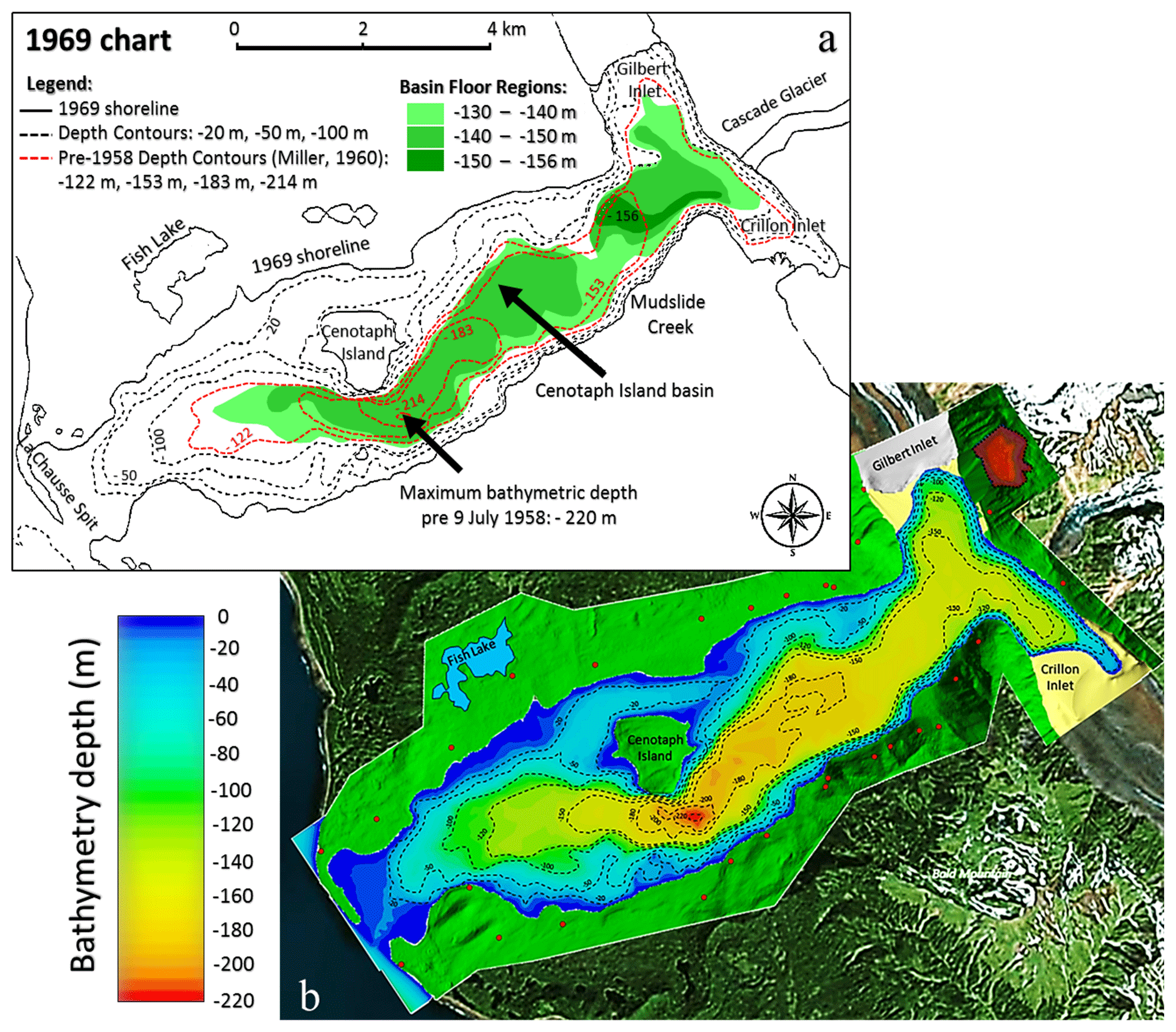
Figure 3(a) The 1969 chart, based on a 1959 survey, highlights the flat bay floor (max. depth about −150, −156 m) relative to the pre-1958 data (dashed red lines; max depth of −220 m) provided by Miller (1960) (modified from Ward and Day, 2010; see Fig. 8). (b) Reconstruction of the pre-1958 Lituya Bay bathymetry based on data from the U.S. Coast and Geodesic Survey, 1926, 1959; digital terrain model (DTM) available from DGGS Elevation Portal of Alaska (background topography from © Google Earth Pro 7.3.2.5776; last access: 24 April 2020).
Since no bathymetry just before the tsunami event is available, a new interpretation of Lituya Bay and the related shoreline before the event is proposed (Figs. 1, 3), starting from the available cartography and the free data provided by the National Ocean Service (Hydrographic Survey with Digital Sounding). The pre-event topography is recreated with a resolution of 5 m.
This work focuses on wave dynamics, wherein a fluid volume moving along the slope represents the trigger process for wave generation and propagation. The intention is to initiate the impulse wave with a comparable impact process. However, reproducing the physical rockslide process is not a target of this study, thus the rheology of the slide is not discussed. A simplified concept of a “denser fluid” in comparison to the seawater is adopted for simulating the impact from the slope. The use of a fluid model, compared to other models like a solid block, gives the possibility of adapting the shape of the moving fluid according to the topographic surface during the collapse process.
First, a detailed analysis of the tsunami formation and run-up in the impact area (near field) is accomplished with the numerical model. A 3D model of the impact area (Gilbert Inlet; Figs. 1c, 2, 4) with a bay geometry simplified as a bucket is reproduced starting from the work done by Basu et al. (2010). Bulk slide volume and density of the observed rockslide are considered for the setup of the denser fluid. The main task of this part is to test the concept of the denser fluid for the impact and to observe wave formation, propagation, and run-up after the impact of the denser fluid into the waterbody.
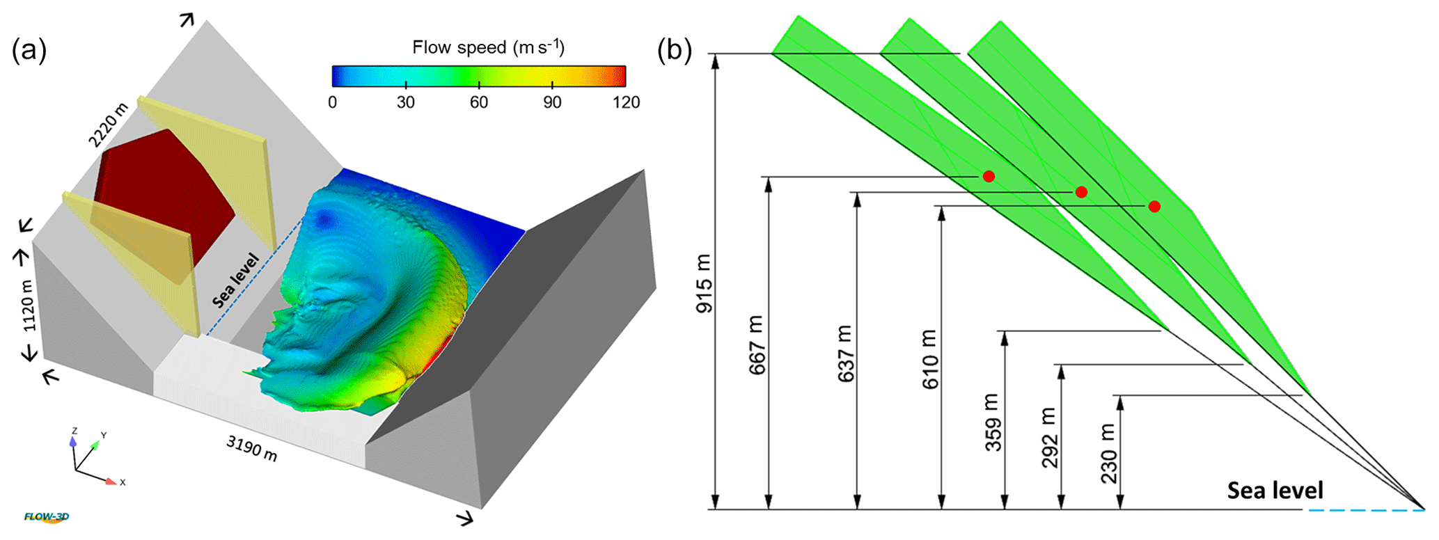
Figure 4(a) Configuration of the bay head at Gilbert Inlet used for concept model analysis (for a slope angle of 45∘). The initial position of the impacting fluid (brown), the glacier (white), and the two constraining walls are shown. The wave propagation and flow speed contours (magnitude of the velocity considering all the vector components) before impacting the opposite slope are illustrated (simulation time =32 s). (b) Illustration showing the position of the impacting fluid and its related centre of gravity (red spot) for different slope angles (35∘, −40∘, ).
In a second step, Gilbert Inlet is recreated using the real topographic and bathymetric surfaces. The model is run using three different uniform cell sizes (20, 10, 5 m). The denser fluid shape is readapted to the detachment area topography. Moreover, the model is enlarged to simulate the propagation of the wave along the entire bay (far field, Fig. 5) and to recreate the inundated area and the related trimline. The results change depending on the cell size adopted for the simulation (20 m × 20 m × 20 m,20 m × 20 m × 10 m, 15 m × 15 m× 10 m). An analysis concerning the adoption of different roughness values for the topographic surface (relative roughness: 0, 1, and 2 m) is achieved with the numerical model.
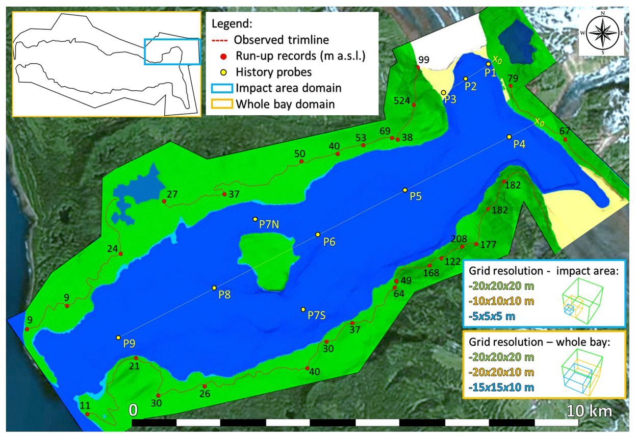
Figure 5Model setup, covering the impact area (light blue rectangle) and the whole bay (orange rectangle); the different adopted grid resolutions are shown. Observation gauges (history probes, shown as yellow points) represent water level gauges; x0 at the impact point and at the shoreline of Cascade glacier represents the origin for the longitudinal distance of the gauges. The observed trimline (dotted red lines) and the documented run-up values along the bay (red spots) are used for model validation (background topography from © Google Earth Pro 7.3.2.5776; last access: 24 April 2020).
2.1 Geomorphological and tectonic setting of Lituya Bay
Lituya Bay is a fjord in southeastern Alaska, originating from glacier retreat (Fig. 1a) 10 000 years ago at the beginning of the current interglacial period (Pararas-Carayannis, 1999), resulting in its present T-shape (Fig. 1b). U-shaped slopes are the main features of the bay, with recent terminal moraine deposits of former Tertiary glaciation periods (Pararas-Carayannis, 1999).
At the head of the bay, the slopes featured very steep walls, ranging from 670 to 1030 m a.s.l. and to more than 1800 m a.s.l. in the Fairweather fault area, about 3 km from Crillon Inlet. Lituya Bay has a length of 12 km and a width ranging from 1.2 to 3.3 km (Fig. 1b), while the entrance is about 300 m in width (Fritz et al., 2001). The northern and southern channels on the side with respect to Cenotaph Island in the middle of the bay are about 650 and 1300 m in width (Fig. 1b). The shores mostly consist of rocky beaches. At the entrance of the bay, La Chaussee Spit (Fig. 1b) represents the terminal moraine resulting from the Last Glacial Period (Pararas-Carayannis, 1999).
The Queen Charlotte and Fairweather faults are situated on the western coasts of Canada and Alaska north of Lituya Bay. They are part of the fault system along the boundaries of the Pacific and North American plates (Tocher and Miller, 1959). The Gilbert and Crillon inlets represent the geomorphological expression of the Fairweather Fault.
2.2 The 1958 Lituya Bay tsunami event
Fritz et al. (2001) report that from 1980 to 2000 four (and probably more) big waves could be verified in Lituya Bay. This occurrence is most likely due to the “unique geologic and tectonic setting of the bay” (Fritz et al., 2001). Miller (1960) reports that several tsunami events happened in Lituya Bay (1853, 1936, and 1958), devastating the forest and reaching an inland run-up of over 100 m a.s.l.
In contrast with many other bays or fjords, the numerous manifestations of tsunamis in Lituya bay are due to several factors. These are (a) its recent environment history (a fjord formed by glacier retreat), (b) the fragile geological and tectonic configuration (steep slopes consisting of fractured rock slopes in a very active fault area), (c) the presence of a great amount of water in the bay and a deep seafloor, and (d) its climate conditions, including intense rain events and periodic freezing and thawing (Miller, 1960).
The earthquake on 9 July 1958, featuring a 7.9–8.3 Mw magnitude, occurred along the Fairweather fault. A rockslide collapsed into the bay at Gilbert Inlet (Fig. 1) (Fritz et al., 2001). Horizontal movements of 6.4 m and vertical movements of 1.0 m were estimated here, as reported in Tocher and Miller (1959). Fishermen that experienced the event spoke of about 1 to 4 min of shaking. The earthquake may have triggered the rockslide (Fritz et al., 2009). The impact of the rockslide generated a huge impulse wave, whose maximum run-up (524 m a.s.l.; Figs. 1c, 2b) is the highest ever recorded in history (Fritz et al., 2001). The wave propagation along the bay resulted in forest destruction and ground erosion (Fig. 1b). Miller (1960) hypothesises that the rockslide is a source of the tsunami by evaluating photographs from the slopes at the Gilbert Inlet before and after the event. He estimates the volume of the main rockslide (30×106 m3) and defines the upper scar limit as being about 915 m a.s.l. (Figs. 1c, 2a).
To be able to distinguish this mass movement from gradual processes and ordinary landslides, Pararas Carayannis (1999) classifies it as “subaerial rockfall”, while Miller (1960) describes it as a mixture between a landslide and a rockfall process according to Sharpe (1938) and Varnes (1958).
Before the catastrophic event, two gravel deltas were located in front of Gilbert glacier (Fig. 1b, c). The rockslide propagated with very high velocity (Ward and Day, 2010), hitting a part of the glacier and the gravel deltas (Miller, 1960). After the event, the glacier front showed a vertical wall (Fig. 2a), since 400 m of ice had disintegrated. At the same time, the deltas had been washed away. Additionally, Ward and Day (2010) describe that the water ran upslope as a surge or splash. The second maximum run-up of 208 m a.s.l. has been identified near Mudslide Creek on the southeastern side of Gilbert Inlet (Fig. 1b). The wave reached an inland distance of 1400 m on the plain in front of Fish Lake (Fig. 1b) on the northwestern side of the bay (Ward and Day, 2010).
Two fishermen eyewitnessed a violent disturbance at the mouth of Gilbert Inlet shortly after the first shaking. They confirmed the rockslide as the trigger of the impulse wave (Ward and Day, 2010). The fishermen estimated the wave's amplitude to be about 15–30 m as it impacted Cenotaph Island (Fig. 1b). On their boats, they additionally experienced a short period with wave heights up to a few metres shortly after the initial wave (Ward and Day, 2010).
2.3 Existing studies on the 1958 Lituya Bay tsunami event
As one of the most studied cases for landslide-generated impulse waves, the Lituya Bay tsunami of 1958 has been and still is of great interest to the scientific community concerning the assessment of natural hazards. Different approaches have been used to reproduce the tsunami, covering analytical studies, physical scale tests, and numerical modelling.
A three-dimensional model of Lituya Bay at a 1:1000 scale was created by Wiegel (1964). Thereby, a run-up of about 3 times the water depth was observed on the opposite slope of the sliding source. Fritz et al. (2001) recreated the 1958 Lituya Bay tsunami in the impact area. They simulated the wave formation and run-up in a two-dimensional physical-scale model as a vertical section of Gilbert Inlet at a 1:675 scale. The results confirm the hypothesis of the rockslide as the source of the impulse wave and the observed maximum run-up. A three-dimensional pneumatic generator for landslide-generated impulse waves was applied by Fritz et al. (2009). The 1958 Lituya Bay rockslide was thereby recreated in a three-dimensional model at a 1:400 scale.
Several studies are based on the use of analytical equations, including those derived from physical-scale test experiments. The main goal of these analyses is to reproduce the wave amplitude and the maximum observed run-up. Concerning the maximum impulse wave height, the results obtained are within the range of 94–162 m (Kamphuis and Bowering, 1970; Noda, 1970; Slingerland and Voight, 1979; Huber and Hager, 1997; Fritz et al., 2004, 2009). Hall Jr. and Watts (1953) and Synolakis (1987) matched the maximum run-up of 526 and 493 m a.s.l., assuming a measured impacting wave height of 162 m and a water depth of −122 m as input (Fritz et al., 2001). Slingerland and Voight (1979) confirmed that a wave height of about 160 m is required to recreate the maximum observed wave run-up. Heller and Hager (2010) applied the impulse product parameter to estimate the main impulse wave characteristics in Lituya Bay. Considering a slide impact speed of 92 m s−1 (Körner, 1976), they predicted a wave height of 179 m based on the wave channel geometry.
Starting from the experiments of Fritz et al. (2001), Mader and Gittings (2002), Quecedo et al. (2004), Weiss and Wuennemann (2007), and Basu et al. (2010) also numerically simulated the 1958 Lituya Bay tsunami event, with a focus on the impact area, by applying the Navier–Stokes hydrodynamics code in two dimensions. Mader (2001) applied the Simulating WAves Nearshore (SWAN) code to model distinct wave trigger mechanisms. These studies stated that a landslide led a tsunami wave to flood Lituya Bay in July 1958 but that it had a mobilised water volume 10 times lower than the volume of the collapsed rockslide. Mader and Gittings (2002) simulated the Lituya Bay tsunami with the Navier–Stokes Adaptive Mesh Refinement (AMR) Eulerian compressible hydrodynamic code (SAGE), which resulted in a maximum wave height of 250 m and run-up of 580 m a.s.l. at the opposite slope.
Pastor et al. (2008) applied a coupling model for displacement and pore pressure together with a generalised plasticity model that describes soil behaviour. Wave propagation is evaluated using a depth-integrated model with fluidised soil rheology. The interaction of the slide and the seawater is simulated with a level-set algorithm that tracks the interfaces between air, water, and solid. They computed a slide impact speed of 110 m s−1, leading to a maximum wave amplitude of 226 m. To simulate the tsunami run-up, Weiss et al. (2009) used a hybrid model approach for the movement of deformable bodies in a U-shaped valley (comparable to Gilbert Inlet). They obtained a maximum wave amplitude of 152 m and a maximum run-up of 518 m a.s.l. Basu et al. (2010) applied the drift–flux model implemented in the CFD software Flow-3D to simulate the landslide-generated impulse wave formation in the impact area of Lituya Bay. Assuming an initial void fraction of 40 % for the rockslide material, they predicted a maximum amplitude of 200 m and a maximum run-up height of around 673 m a.s.l.
The two-dimensional representation of Lituya Bay of Fritz et al. (2001) was also used by Schwaiger and Higman (2007), Chunqi et al. (2016), and Xenakis et al. (2017) in the context of an SPH (smoothed particle hydrodynamics) modelling approach. SPH allows for a better representation and simulation of the landslide material collapse process and its impact on the waterbody.
Ward and Day (2010) developed a new “tsunami ball approach” to simulate the impulse wave formation and propagation along the whole Lituya Bay. They predicted a wave height up to 150 m in the impact area and a run-up height of 500 m a.s.l. They considered a dual source for the tsunami event: the subaerial rockslide and a huge amount of subglacial sediments released in the bay after the rockslide impact in the waterbody. The resulting trimline is overestimated by the dual-source approach, but only the subaerial rockslide as an impulse wave trigger was not enough to explain the whole flooded area along the bay. González-Vida et al. (2019) applied a finite-volume Savage–Hutter shallow water coupled numerical model (HySEA). The resulting numerical simulations succeeded in reproducing most of the features of the tsunami event.
3.1 Pre-event bathymetry and topography
Digital data and cartographic material concerning the bathymetry and topography of Lituya Bay dated before and after the tsunami event are available. None of these data are close enough to describe the exact configuration of the bay shortly before 9 July 1958.
The 1926 and 1940 bathymetry surveys (U.S. Coast and Geodesic Survey, 1926, 1942) show that the northeastern limit of Lituya Bay has a U-shaped valley with steep slopes and a wide flat seafloor, which constantly increases its depth until a maximum of −220 m a.s.l. on the southern side with respect to Cenotaph Island (Pararas-Carayannis, 1999) and then decreases in the direction of the sea. In the area close to the bay entrance, the bay floor is −10 m a.s.l. on average.
Miller (1960) was the first after 1958 to describe the bay before the tsunami event (Fig. 1c). He describes the area between Cenotaph Island and Gilbert Inlet as a wide expanse with depths between −150 and −220 m a.s.l. He highlights the presence of two deltas on both sides in front of Gilbert Inlet. Miller (1960) mapped the pre-event topographic and bathymetric contours. In the post-1958 surveys, these areas and deltas are not present (Ward and Day, 2010). The 1969 chart obtained from the 1959 survey (U.S. Coast and Geodetic Survey, 1969) shows a flat bay floor (green zones in Fig. 4a). A ridge divided the bay floor into two sub-basins: a smaller one southeast of Gilbert Head (−156 m maximum depth) and a larger one on the south front of Cenotaph Island (−150 m maximum depth). A third survey published in 1990 (U.S. Coast and Geodetic Survey, 1990) creates the possibility of estimating the sedimentation rate over time. The two charts, the first from 1942 to 1969 and the second from 1969 to 1990, differ completely (see Fig. 8 in Ward and Day, 2010). The northeastern sub-basin in front of Gilbert glacier is filled by sediment. The bay floor decreases constantly between Gilbert Inlet and the basin in front of Cenotaph Island. Ward and Day (2010) estimated that 3×10⁸ m3 of material was discharged into the bay after the tsunami event, filling it until the −130 m depth contour, resulting in a 70 m thick deposit. From the previous considerations, they propose a hypothesis to justify the whole infill of the bay between 1926 and the 1958 tsunami event. Given that (i) the sedimentation rate is assumed constant during the last century; (ii) in 1936 a landslide collapsed into the bay (where the generated wave was a tenth of the size of the 1958 tsunami; Miller, 1960); (iii) the 1958 rockslide contained 3–6×10⁷ m3 of material (10 %–20 % of the total infill volume); and (iv) soil, subsoil, and bedrock have been eroded by the wave (about 4×10⁶ m3; Miller, 1960), they suggested that the remobilised sediment located under Gilbert glacier contributed to infilling the bay floor during the tsunami event. The volume generated from the displacement of the deltas in front of Gilbert glacier has thereby not been considered.
All of these considerations are useful to give a good interpretation of the bay pre-event configuration (Fig. 3b). The bathymetric data used for this study are provided by the National Ocean Service: Hydrographic Surveys with Digital Sounding. In particular, data from Survey ID: H08492 (1959) are used as reference bathymetry after the event since this survey is the closest to the 9 July 1958 tsunami event, as well as data from Survey ID: H04608 (1926) the closest survey prior to the event. The survey from 1926 does not feature a sufficient spatial resolution to provide an acceptable bathymetry in the whole bay. Nevertheless, it provides sufficient information on the pre-tsunami bathymetry in the areas at Gilbert Inlet and south of Cenotaph Island. As mentioned in Ward and Day (2010), the infilling material after the 1958 event covers an area between the −120 and the −130 m depth contours. In the map, contour lines defined by Miller (1960) (dashed red lines in Fig. 3a) from a depth of −122 to −220 m show the bay bathymetry before the infill. From these considerations, the elevation points from the Survey ID: H08492 (1959) are taken as representative of the shallower part of the bay floor (from the surface to −120 m depth). Below −120 m depth, the elevation points from the Survey ID: H04608 (1926) are considered to be representative of the deeper area of the bay floor. Due to limited data, the contour lines defined by Miller (1960) are used to better reproduce the shape of the bay floor. For the flatter areas, lines are set between different elevations points to allow a more accurate interpolation for the bay floor surface reconstruction. The delta in front of Gilbert glacier (Fig. 3a) is reproduced considering the information given by Miller (1960).
The pre-event topographic surface is reproduced starting from the current digital terrain model (5 m resolution) available from the DGGS Elevation Portal of Alaska. Contour lines of 5 m are used to recreate the topography. Contour lines of 1 m are also used to highlight some details that influence the estimation of the flooded area (such as steeper slopes, hills, or specific topographic changes). The observed trimline and the run-up records (red spots in Fig. 3b) are used as references to define the required spatial extent of the model topography.
Manual modifications of the DTM are provided at the Gilbert and Crillon Inlet locations in order to recreate those geomorphological elements that have been displaced and washed away during the landslide impact and wave formation. Crillon Inlet, Gilbert glacier, and the deltas in front of them are recreated starting from the descriptions provided by Miller (1960) and the available cartography (see Fig. 16 in Miller, 1960). Miller (1960) reports a scarred area, pre-dating the tsunami event, located north of the maximum observed run-up (Fig. 2b). He only identifies a little scar exactly under the maximum run-up that could have been formed after the tsunami event. The pre-event shoreline is also reproduced starting from the descriptions provided by Miller (1960).
The bathymetric and topographic surfaces are recreated and exported to stereolithography files (STL) via Rhinoceros 6 software (https://www.rhino3d.com/, last access: 24 March 2020).
3.2 Model setup and computational details
3.2.1 Solver methodology
For computational modelling the CFD software Flow-3D (Harlow and Welch, 1965; Welch et al., 1966; Hirt and Nichols, 1981; Flow Science Inc., 2018) is applied. Its solver is based on a finite volume formulation in a Eulerian framework. The partial differential equations express the conservation of mass, momentum, and energy of the fluid in the computational domain. The software enables the possibility of simulating two fluid problems, i.e., incompressible and compressible flows, as well as flow conditions at highly different Reynolds numbers (laminar, turbulent). Flow-3D solves the Reynolds-averaged Navier–Stokes equations (RANS) adopting the fractional area–volume obstacle representation (FAVOR) (Hirt and Sicilian, 1985) and the volume of fluid (VOF) (Hirt and Nichols, 1981) method.
The Reynolds-averaged Navier–Stokes and the continuity equations are expressed as follows (Hinze, 1975):
where is the Reynolds-averaged fluid velocity, p is the Reynolds-averaged pressure (divided by the density ρ), v is the kinematic viscosity of the fluid, and T is the Reynolds-stress term (which include the reaction of the turbulent motion on the mean stresses) (Hinze, 1975).
The VOF method is a two-phase solution where the grid includes both water and air. With this approach, every cell in the mesh has a fraction of water (F) that is equal to 1 when the cell is fully water-filled and 0 when it is air-filled. In cases between 0 and 1, the cell comprises the free water surface. A transport equation is thus considered as follows (Rady, 2011):
where u, v, and w are the components of the fluid velocity in the x, y and z directions, respectively.
The FAVOR algorithm (Hirt and Sicilian, 1985) allows for the definition of solids within the orthogonal computational grid and computes areal and volumetric fractions of blocked volumes of each computational element. A set of turbulence models is implemented in order to cope with the problem in the context of the RANS equations and to simulate turbulent flow conditions. For this work, the Renormalization Group (RNG) model (Yakhot and Smith, 1992) is used, which adopts statistical models to calculate the two model parameters: the turbulent kinetic energy and the turbulent kinetic energy dissipation rate.
Several tools and parameter modules are useful to simulate a body sliding along a slope and impacting a water basin, depending on which kind of gravitational process is simulated (rockfall, rockslide, rock avalanche, or snow avalanche). Using a denser fluid with respect to the seawater for the sliding mass is a suitable concept for those gravitational processes that behave more like a fluid during their collapse and run-out processes. The use of this concept to qualitatively recreate the sliding process (similar to the model described by Miller, 1960, and Fritz et al., 2001) is a well-suited approximation for the impact modelling of the Lituya Bay event. Both the first-order and the second-order approaches for the density evaluation implemented in Flow-3D are adopted to simulate the two fluids and their interaction. These models (first-order approximation to density transport equation, and second-order monotonicity preserving approximation to density transport equation) calculate a distinct density transport equation and perform the motion of two different fluids (of different densities) in the domain, thereby simulating two fluids together with a free surface (Flow Science Inc., 2018). The density varies due to the initial and compressibility conditions.
All simulations are run with the same computational resource with the following hardware components.
-
Processor: Intel® Core™ i7-3820 CPU 3.60 GHz;
-
RAM: 32 GB;
-
System type: 64-bit Operating System;
-
Graphics card: GeForce GTX 6602 (Integrated RAMDAC, total available memory 4096 MB);
-
Number of core license tokens checked out: 8 (Flow-3D parallel license code).
3.2.2 Denser fluid setup
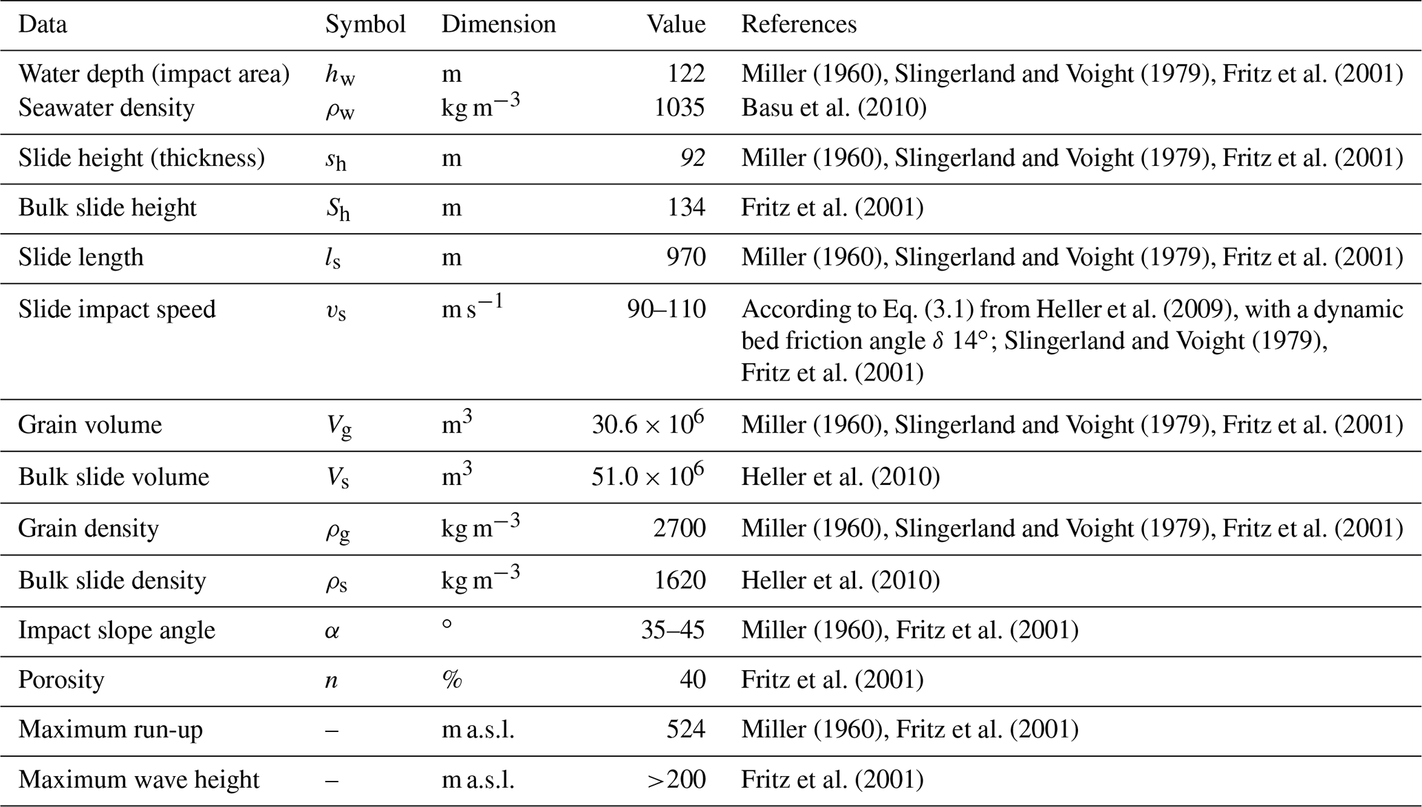
The cliff material consists mostly of amphibole and biotite schists with an estimated density of the undisturbed rock of 2700 kg m−3 (Table 1). The sliding mass dimension before the collapse is well known. The thickness of the slide has been defined by Miller (1960). The mass of the rockslide is described as a rock prism with a triangular shape (along a vertical section) with a width varying from 730 to 915 m (Miller, 1960; Slingerland and Voight, 1979; Fig. 1c). The length results in 970 m along the slope (Slingerland and Voight, 1979, Table 1). The maximum thickness results in 92 m; the centre of gravity is located at 610 m elevation (Miller, 1960; Table 1, Fig. 1c). Miller estimated the volume of the sliding mass to be about 30.6×10⁶ m3 with an elevation from 230 to 915 m a.s.l.
Table 1Summary of the governing parameters of the 1958 Lituya Bay tsunami event and related references.
Due to the lack of data available, the rheology of the rockslide is difficult to describe. Limited information has recently been provided in the literature (Quecedo et al., 2004; Schwaiger and Higman, 2007; Pastor et al., 2008; Mao et al., 2017; Xenaksis et al., 2017), where artificial rheological parameters are obtained empirically following computational experiments or resulting from back analysis of similar rockslides. Xenaksis et al. (2017) describe the slide phase as a mixture of different materials with different properties (rock, soil, ice, and vegetation), where non-Newtonian shear-thinning rheological properties are assumed. Mao et al. (2017) adopted a rheological model as a non-Newtonian viscoplastic fluid model in order to recreate a deformable fluid-like slide body.
Since in this case there is a lack of directly observed data, and since a proper setup and validation of the rockslide model with the software Flow-3D is possible, a simple concept of a denser fluid is adopted. The bulk slide volume and bulk slide density, 51.0×10⁶ m3 and 1620 kg m−3, respectively, are used for the denser fluid simulation (Table 1). As was done in Fritz et al. (2001), the reduced bulk density of 1620 kg m−3 considers a void content of 40 % (Table 1). The porosity parameter used is based on data from debris flows observed in the Alpine region (Tognacca, 1999). This is not entirely representative of the real rockslide material but gives an appropriate approximation for rockslide properties.
3.2.3 Model concept analysis
A 3D model of the Lituya Bay topography, idealised as a bucket shape, is assumed for the model concept analysis (Fig. 4a), starting from the information provided by the 2D numerical simulations proposed by Basu et al. (2010), which summarise the experiment of Fritz et al. (2001). The simulation time is set to 60 s. The terrain model and the computational domain are presented in Fig. 4a.
Different slope angles of 35, 40, and 45 ∘ are set to verify the influence of the impact angle on the impact speed (Fig. 4b). Despite the change in inclination, the difference in heights is maintained at equal levels in all simulations, thus the geometrical setup is done in such a way that this difference is measured from the sea level to the upper edge (915 m a.s.l.) of the denser fluid at its initial position (Fig. 4b). To ensure the same volume and shape, the centre of gravity (as well as the lower edge of the denser fluid) is at different heights for different slope situations.
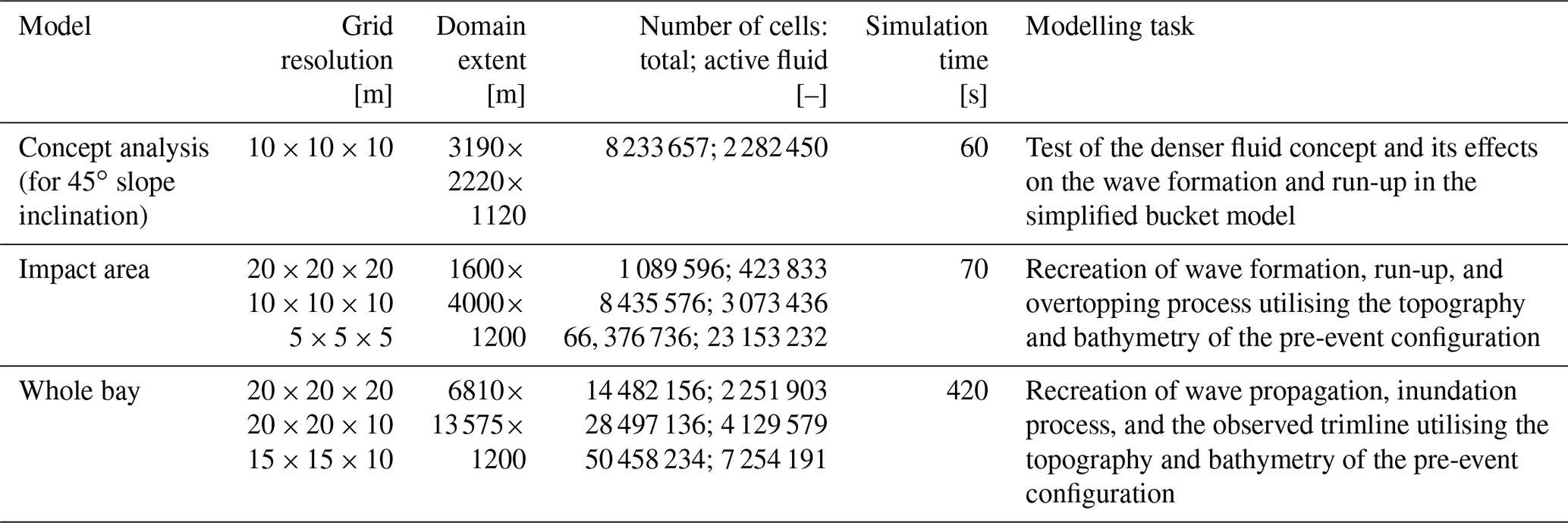
The computation domain has its origin located on the bay floor, assumed to be −122 m below sea level (Table 2). An orthogonal grid comprising a uniform cell size of 10 m is defined for these models. The grid includes the air space above the bay between the headlands to accommodate the waves according to the VOF algorithm (Basu et al., 2010). In order to reduce the number of active cells in the domain (thus saving computational memory and improving model stability), a solid body occupying higher air cells (where no fluid is expected to occupy space during the simulation) is set as a domain remover. This is applied the same way for the model concept analysis as for the formation and propagation models, in a way that the limits of the active domain correspond to the limits of the recreated topography (Fig. 5).
The boundaries are specified as the outflow on the free sides of the idealised topography to allow the fluid to flow out of the model without any kind of interaction or reflection. The extent of the flow domain is set in such a way that the fluid interacts mostly with the boundary that represents the bay floor and inland slopes (left and right boundaries).
The presence of the glacier, and possible virtual walls, to constrain the fluid during its movement along the slope, is also considered (Fig. 4a). With regards to the evaluation of the modelling concept, it is expected that the impact velocities stay within the interval 90–110 m s−1 (Table 2).
The initial fluid in the bay represents typical seawater conditions and features a density of 1035 kg m−3 (Table 1).
3.2.4 Modelling of the impact area and the whole bay
Further simulations in the impact area (near field) include the topography surface and the recreated bathymetry (Fig. 5, Table 2). The simulation time is 70 s. Different uniform cell sizes are set up for these simulations (20, 10, and 5 m) in order to verify the accuracy of the results based on the grid resolution (Table 2). The simulation domain extends to 1600 m × 4000 m in the x–y direction and 1200 m in elevation. The same boundary conditions as those used for the model concept analysis are set for these simulations. The denser fluid shape is redefined starting from satellite images and cartographic material pre-event. The resulting volume is readapted to the detachment area. The maximum used slide thickness of 134 m is equivalent to 1.4 times the thickness of 92 m provided by Miller (1960). This increase of 40 % in thickness was also considered by Fritz et al. (2001). They adopted this rise in slide density to compensate for the void fraction current in granular flow to match the slide mass-flux per unit width.
For the impulse wave propagation along the whole bay (far field), the domain extends to 6810 m × 13 575 m in the x–y direction and 1200 m in elevation (Fig. 5, Table 2). The simulation takes 7 min. Uniform and non-uniform cells of different sizes are set up 20 m × 20 m × 20 m, 20 m × 20 m × 10 m, and 15 m × 15 m × 10 m). At the domain limits, at the Gilbert and Crillon inlets, and at the seaside, the outflow boundary condition is set to allow the wave to flow out from the model domain.
Control points (Fig. 5) representing specific records of run-up are set in order to validate the results. Several observation gauges (history probes) are set along the entire model domain to achieve information regarding impact time; impact speed (defined as the one of the centre of gravity of the sliding mass entering into the waterbody; Evers et al., 2019); wave propagation speed; and characteristics such as water surface elevation (or wave amplitude), flow speed (magnitude of the velocity vector, resulting from the vector components x, y, and z of the fluid at a specific point in the 3D domain), and their trend in time. In the impact area, probes P1, P2, and P3 are located along the main wave flow direction (Fig. 5) for a streamwise distance from x0 of 45, 688, 1342 m, respectively, from the impact point. Other history probes are set parallel to the bay length (Fig. 5), starting in front of the delta corresponding to Cascade glacier for a streamwise distance from x0 of 600 m (P4), 3100 m (P5), 5600 m (P6), 6600 m (P7N/P7S, both located laterally with respect to Cenotaph Island), 8100 m (P8), and 10600 m (P9).
The surface roughness in Flow-3D consists of two components. The first results from the pre-processing phase of the considered solid structures (STL files) with the FAVOR method. Depending on the mesh structure and grid resolution, it features divergences from the original solid structure. The computational geometry usually features a rougher surface than the solid structure in cases where the mesh orientation does not fit perfectly with the surface slope. Furthermore, a second additional roughness parameter, defined as equivalent grain roughness (m), can be set for each solid structure to consider, for example, vegetation.
The computations in this study are mainly set up with the equivalent grain roughness equal to 0 m for the topographic surface. In order to verify the influence of the vegetation on the inundation process and the trimline definition, simulations with values of 1 and 2 m of roughness are set up for simulations with a grid resolution of 15 m × 15 m × 10 m.

Figure 6Impact speed distribution vs. time for the impacting fluid considering different slope angles of (a) 45∘, (b) 40∘, and (c) 35∘. The lower and upper limits represent a reasonable speed interval for the centre of gravity of the deforming fluid when entering the waterbody (from Eq. 3.5 in Evers et al., 2019, with a dynamic bed friction angle δ of 0 and 14∘).
4.1 Evaluation of the denser fluid concept
Several preliminary simulations are accomplished with the numerical model, in order to test the concept of the denser fluid with respect to the seawater density for the impacting fluid. Different configurations are investigated: (a) different slope angles (35, 40, 45∘), (b) absence or presence of Gilbert glacier (as a vertical wall of 100 m a.s.l.), and (c) use of virtual walls to constrain the denser fluid during its movement along the slope. This is done to observe the reaction of the wave depending on the changes in these options, in comparison to the simple bucket shape.
The whole process reflects what resulted from the experiment of Fritz et al. (2001), which describes the high velocity of the slide impact process with the following two main steps: (a) the impact of the slide, with the emergence of cavity effects and generation of the impulse wave, and (b) the collapse of the air cavity together with the mixing process of the different components. The formation of a large air cavity after the initial impact is well observed in the computational model.
The results of the model concept analysis are discussed as follows.
-
The denser fluid reaches the waterbody within 10–14 s. The maximum impact speed varies between 92–114 m s−1 depending on the modelled impact angle (Fig. 6c). The denser fluid does not act as a non-deformable body during the moving process along the slope. Thus, this deformation has a considerable influence on the impact speed. In Fig. 6, the fluid speed during the impact process is shown for every considered slope angle. An upper and a lower limit (dashed black lines) define a reasonable speed interval for the centre of gravity entering into the waterbody (values obtained from equation 3.5 of Evers et al., 2019, with a dynamic bed friction angle δ of 0 and 14∘).
-
The presence of the virtual constraining walls does not significantly influence the impact speed, although it avoids the mass spreading along the slope during its movement.
-
The impulse wave is formed and reaches its maximum height after 9–10 s following the impact, with a wave amplitude ranging between 203–220 m.
-
The presence of the constraining walls increases the wave amplitude by 5 to 15 m. This means that the shape of the denser fluid (fluid thickness), as it is constrained by the walls at the impact, influences the wave characteristics more than the impact speed. The presence of the glacier does not influence the wave formation.
-
The additional presence of the glacier, together with the constraining walls, affects and increases the impulse wave just before the impact on the opposite headland (20 s after the slide impact). Here, the wave amplitude ranges between 156 and 217 m. It is observed that the wave has no possibility to complete its breaking process, hitting the opposite headland very violently and starting its run-up process along the slope.
-
Different maximum run-up values result from different model configurations. They overestimate the observed one, ranging from 570 to 790 m a.s.l. between 36–38 s after the slide impact and 16–17 s after the wave hits the opposite headland. Once the maximum run-up is reached, a backflow of the wave is observed.
-
Closer run-up values of 524 m a.s.l. are found for calculations considering the simple bucket shape of the bay, without the presence of the glacier and walls. Considering these two elements in the model, the maximum observed run-up is highly overestimated.
-
It is noticed that the use of different order approaches for density evaluation influences the interaction between the two fluids. With the first-order approach, the mixing process leads to a change in density of the denser fluid from 1620 to about 1250 kg m−3. With the second-order approach, the density changes to 1400 kg m−3. In both cases, a part of the denser fluid runs up a short distance on the opposite slope. The order of the density evaluation approach does not influence the wave characteristics.
The main aim of several authors was to reproduce the impulse wave formation and reach the observed run-up. Provided that the wave run-up could reproduce this value (and consequently the backflow), it could be assumed to have obtained a reliable result and a good reproduction of the 1958 Lituya Bay tsunami event. However, this is not properly correct when taking into consideration the complete run-up process. Actually, the wave did not stop at 524 m a.s.l. but overtopped the hill crest and continued to flow diagonally along the slope to the other side for a distance of about 1 km before re-impacting the sea (Figs. 1c, 2b). An overestimation of the maximum run-up, in these simplified simulations, makes sense for allowing the further overtopping at the hill crest. More “power” is needed to reproduce the phenomena and what has been observed in the whole bay. For the model concept with a topographic surface, the presence of the glacier (and walls to constrain the denser fluid during the movement along the slope) might be necessary to recreate the impulse wave formation and run-up at the head of Lituya Bay.
4.2 Wave formation and run-up – near field
A topographic and bathymetric surface of the impact area is set up and the shape of the denser fluid is readapted to the detachment area (Figs. 5, 7a). What changes here with respect to the model concept analysis is that (a) the slope angle is not constant but ranges from 45∘ at higher elevation to 35∘ at the shoreline, and (b) the volume of the seawater is involved in the numerical model since the deltas where not considered in the simplified simulations (about 1.73×10⁶ m3 of seawater compared to 3.34×10⁶ m3 in the model concept analysis). This can have a significant influence regarding the water volume involved in the wave formation and run-up.
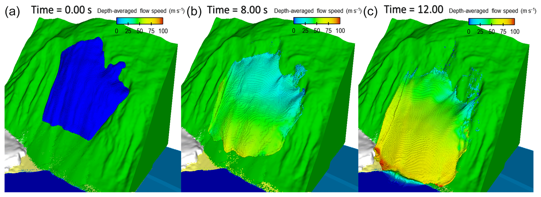
Figure 7Fluid model at (a) 0 s, (b) 8 s, and (c) 12 s impacting the sea, coloured by the depth-averaged flow speed in (m s−1) with a range of 0–100 m s−1. Uniform grid resolution of 5 m.
The main aim of this part of the work is to investigate the wave characteristics after the impact of the denser fluid, in order to simulate not only the maximum run-up but also the overtopping process and the flow path along the slope on the other side with respect to the Gilbert Inlet and to recreate the related trimline.
The detachment area, where the rockslide failed, is confined on the left side from the topographic surface, while on the right side two scar channels are presented (Figs. 2a, 7a). These are related to other smaller rockslides that occurred during the earthquake but were not involved in the impulse wave formation (Miller, 1960). For this reason, a constraining wall (invisible in the images, Fig. 7) is set only on the right side with respect to the rockslide described by Miller (1960). A simulation without the wall is also set up to observe the eventual fluid collapse and impact process.
The results obtained (Fig. 8) vary according to the adopted uniform grid resolution (20, 10, 5 m) (Fig. 5). The best fit with the observed maximum run-up in the impact area can be achieved using a uniform grid resolution of 5 m.

Figure 8Wave formation and propagation in the impact area using the second-order approach for the density evaluation. Observation gauges P1, P2, and P3 are set to verify the water surface elevation and flow speed. Their trends are shown in the graphs for different grid resolutions (R: 5, 10, 20 m). More accurate results are obtained using the grid resolution of 5 m (sky-blue line, R5).
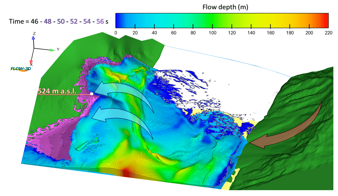
Figure 9Impulse wave run-up on the opposite slope. At the 46 s time step the wave reaches the maximum observed elevation of 524 m a.s.l. (flow depth contours). A part of the wave body overtops the hill and proceeds on its path in a diagonal direction with respect to the slope gradient (shown by the different shades of purple for the time steps of 48, 50, 52, 54, and 56 s).
A description of the wave formation and run-up resulting from the simulation with 5 m grid resolution and the adopted second-order approach for the density evaluation is provided below. This model takes 30 h to run.
-
0–15 s. The denser fluid reaches the sea after 10 s with a maximum impact speed of 93 m s−1 and a maximum thickness of 79 m (P1 – x0=45 m, Figs. 7c, 8a). The depth-averaged flow speed varies from 40 m s−1 in the upper part to 90 m s−1 in the lower part of the fluid during the movement (Fig. 7).
-
15–30 s. After 24 s after the release of denser fluid, the maximum estimated wave amplitude results in 208 m with a flow speed of 78 m s−1 (P2 – x0=688 m, Fig. 7b). Slightly further (x0=885 m), the wave maintains its height to start its breaking process. A part of the wave also flows on the glacier. The wave front runs up the delta and the following slope (Fig. 7c).
-
30–35 s. The whole wave crashes on the opposite headland after 30 s following the denser fluid release (20 s after the impact), with a variable water surface elevation of 129–147 m a.s.l and a flow speed between 50–70 m s−1 (P3 – x0=1342; Fig. 7c). The wave-breaking stage is not complete, it partially breaks when it flows on the delta.
-
35–50 s. The wave runs up towards the headland and the scars located upon the delta. The maximum observed run-up (524 m a.s.l.) is reached after 46 s (36 s after the denser fluid impact, Fig. 9) with a flow depth of 4–10 m and a flow speed of 12 m s−1. A part of the wave body overtops the hill crest, but a backflow is also observed.
-
50–70 s. The wave flows in a diagonal direction relative to the slope, with a depth-averaged flow speed of 50–70 m s−1. The wave reaches the seaside 8 s after the maximum run-up (54 s from the denser fluid release, Fig. 9). The flow depth is about 15 m with a flow speed of 70 m s−1.
During the collapse process, it is noticed that the left part of the denser fluid is well constrained by the actual topography (Fig. 7b, c). Avoiding the wall on the right side, the mass largely spreads and collapses on the glacier, losing a great amount of volume involved in the impact process and decreasing the wave formation. The presence of the wall constrains the denser fluid on this side and allows it to collapse in the waterbody. In addition, Gilbert glacier acts as a constraining wall, and the delta in front of the glacier acts as a ramp.
The maximum wave amplitude of 208 m is located upon the terminal front of the delta on the bay floor (where the history probe P2 is located; graph in Fig. 8b). Here the wave celerity is estimated to be 55 m s−1 (from Eq. 2.2; provided by Heller et al., 2009). The wave starts to break because of its interaction with the decreasing bay floor depth. Fritz et al. (2001) observed the maximum wave height (>200 m) at x0=600, while at x0=885 they reconstructed a wave height of 152 m.
The presence of the scar area on the right side of the maximum run-up has a key role in the run-up process, since it allows the wave to run up along a channel (Fig. 9) and reach the elevation of 524 m a.s.l. This observation supports the topography description provided by Miller (1960). Despite the reproduction of the expected overtopping over the hill and the flow process on the other side of the slope, the resulting trimline appears to be underestimated compared to the observed one (light blue in Fig. 12b).
Additionally, if 524 m a.s.l. is the maximum run-up elevation observed from the trimline, it is not clear in the scar area on the right side, since there is no evidence of a forest trimline. With regards to the simulation results, it appears that the maximum run-up reached an elevation up to 600 m a.s.l. in this part of the slope.
4.3 Impulse wave propagation – far field
The aim of these simulations is to reproduce the wave propagation along the bay, to understand how the waves interact and inundate the inland area, and to recreate the actual trimline. For the wave propagation, only the second-order approach for the density evaluation has been used. Observation gauges for water level measurement allow more insights into the wave characteristics during the propagation and to observe the wave attenuation along the bay to the seaside (Fig. 5).
The results obtained from the simulations vary depending on the resolution of the computational grid. A description of the wave propagation and inundation resulting from the simulation with 15 m × 15 m × 10 m grid resolution is provided (details are referred to the primary wave front). The model takes 165 h to run completely.
-
0–60 s. Over the impact area, the wave starts to propagate, resulting in a water surface elevation of 40 m a.s.l. and a flow speed of 9 m s−1 at P4 (x0=600, Fig. 10a).
-
60–120 s. The wave propagates in open water; at P5 (x0=3100, Fig. 10b) a water surface elevation of 39 m a.s.l. and a flow speed of 19 m s−1 are recorded due to the amount of water flowing down the slope with high velocity. An impact on the southern side of the bay in front of the Gilbert Inlet is observed, where a secondary wave front is generated due to reflection. The primary wave front reaches the Mudslide Creek delta and floods the inland area with a depth-averaged flow speed of 20–30 m s−1. The second highest run-up results are overestimated with 233 m a.s.l. about 94 s after the release of the denser fluid (the observed one is 208 m a.s.l.).
-
120–200 s. The wave splits into two fronts approaching and impacting Cenotaph Island (water surface elevation of 22 m a.s.l. and 8 m s−1 flow speed recorded at P6, x0=5600, Fig. 10c). On the southern side, the wave slightly slows down due to the attenuation process, with a water surface elevation of 19 m a.s.l. and a flow speed of 5 m s−1 at P7S (x0=6600). The steep slopes on the southern side of the bay are completely flooded by the wave (Fig. 10d). On the northern side of the island, where the bay floor gets more shallow (depth 20–40 m) and narrow, the water surface elevation results in 15 m a.s.l. with a speed of 7 m s−1 at P7N (x0=6600, Fig. 12d). This is due to a breaking process.
-
200–280 s. Due to diffraction, the waves turn around the island and flood the western side of Cenotaph Island. The wave front from the southern channel comes first, as observed at P8 (x0=8100, Fig. 10d and e) resulting in a flow speed of 4 m s−1 and a water surface elevation of 10 m a.s.l. The flatter northern side of the bay is flooded (Fig. 10e).
-
280–340 s. The wave reaches the maximum distance of 1400 m, flooding the area in front of Fish Lake with a depth-averaged flow speed of 10–25 m s−1 and a corresponding water surface of 15–5 m from the ground (Fig. 10f). The wave approaches the mouth of the bay, resulting in a water surface elevation of 13 m a.s.l and a flow speed of 5 m s−1 at P9 (x0=10 600, Fig. 10f). The second wave front reaches the first one, resulting in a long period wave; it takes 180 s to pass over the history probe P9 (from 240 s to the time limit of the simulation, 420 s).
-
340–420 s. After 340 s following the release of the denser fluid, the wave reaches the seaside, completely flooding La Chaussee Spit and the nearby areas with a depth-averaged flow speed of 10–20 m s−1.
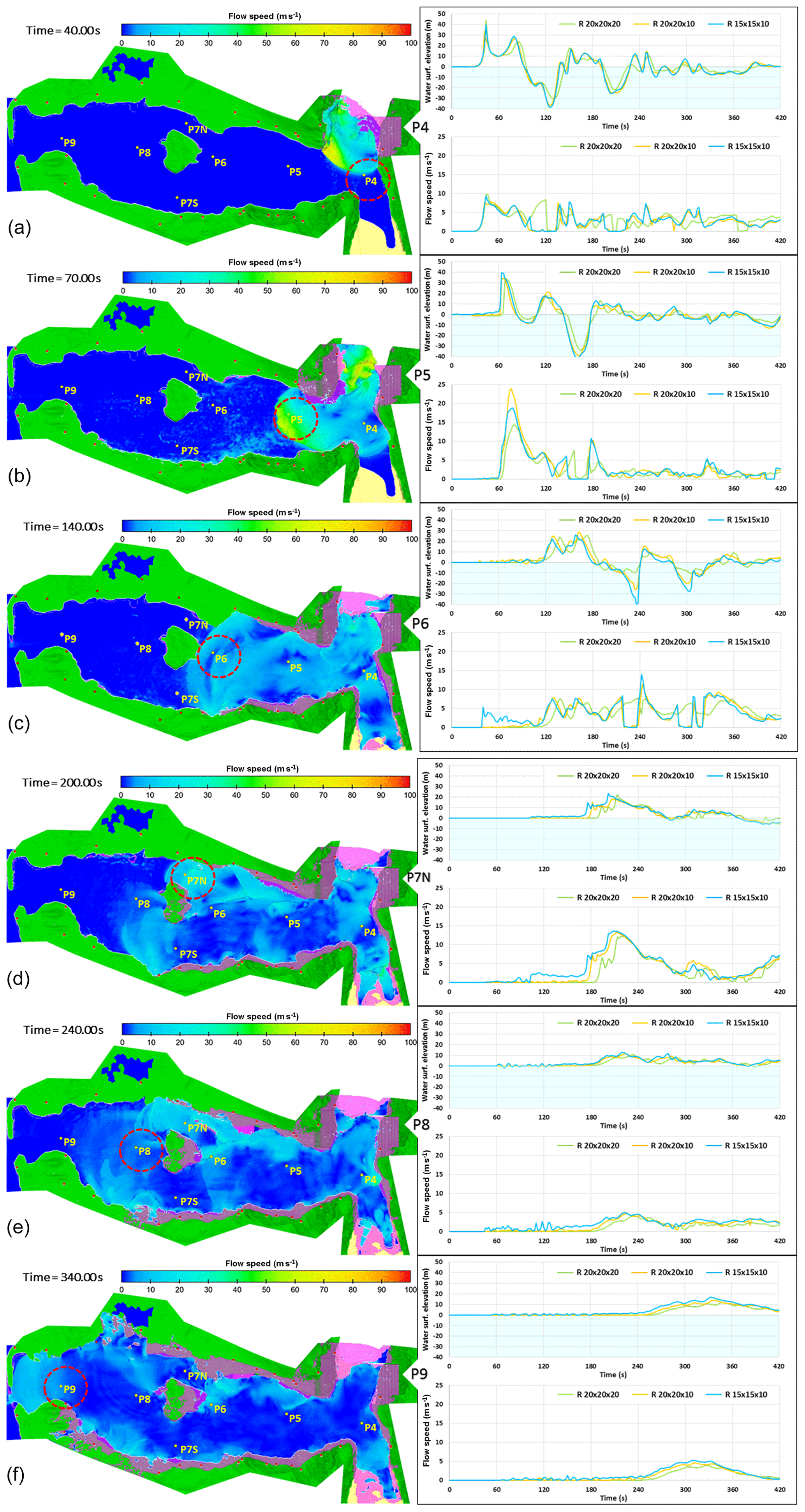
Figure 10After the fluid impacts into the sea, the wave propagates and floods the inner land along the bay. The images show the flow speed at (a) 40 s, (b) 70 s, (c) 140 s, (d) 200 s, (e) 240 s, and (f) 340 s. Different observation gauges are set to check the wave attenuation during wave propagation. The trend of the water surface elevation and flow speed are shown in the graphs for the related observation gauge, adopting different non-uniform grid resolutions (R: 20 m × 20 m × 20 m, 20 m × 20 m × 10 m, and 15 m × 15 m × 10 m). The purple colour of the inland are represents the inundated areas when the wave propagates (the simulation video is listed in the Data Availability section below).
The main wave is mainly responsible for the forest destruction, but secondary reflected waves along the bay also contribute to the observed trimline. A clear example is the wave reflected from Mudslide Creek impacting the opposite northern slope of the bay at 140 s (Fig. 10c). Other secondary wave fronts spread from the bay head due to several reflections of the backflow in front of the Gilbert Inlet.
In Fig. 11a, the wave propagation for the primary wave front is illustrated. The reported values represent a mean value of wave propagation speed (from 40 to 17 m s−1) for each space interval, starting from the records provided by the gauges located along the bay, considering the wave front position at the time of its passage upon every singular gauge (Fig. 11b) and adopting flow path lines for distance estimation. These reflect the interaction of the impulse wave with the bay floor (thus local changes in water depth) and the bay shape. Higher values of the mean propagation speed are estimated between x0 (impact location) and P8, ranging between 36–40 m s−1, and vary in response to the local change of the water depth (−150–220 m), inducing slight local increases or decreases in the mean propagation speed. A value of about 60 m s−1 is observed between P4 and P5, probably due to the water flowing down the slope, whose impact into the sea induces a local acceleration of the wave in open water, and thus a higher propagation speed. Cenotaph Island and the northern shallower bay floor represent obstacles that induce a slowdown for the wave propagation speed. Due to the sudden shallowing of the bay floor (about −20 m in water depth) wave speed decreases drastically between P6 and P7N (28 m s−1). A general decrease in the propagation speed is observed from P7S to the mouth of the bay (from 33 to 17 m s−1), related to the progressive decrease in the water depth (from –160 to –10 m). The wave attenuation process, in terms of wave amplitude (from 40 to 18 m), proceeds from the head of the bay until the seaside. Dashed lines represent the secondary wave in time. Its role becomes relevant after gauge P6: the second front approaches the first one evolving in a whole wave body between P9 and La Chaussee Spit (C.S. in the graph), inducing an increase in the wave amplitude (from 13 to 18 m) before a breaking process (due to the high shallowing of the bay floor compared to the wave amplitude).
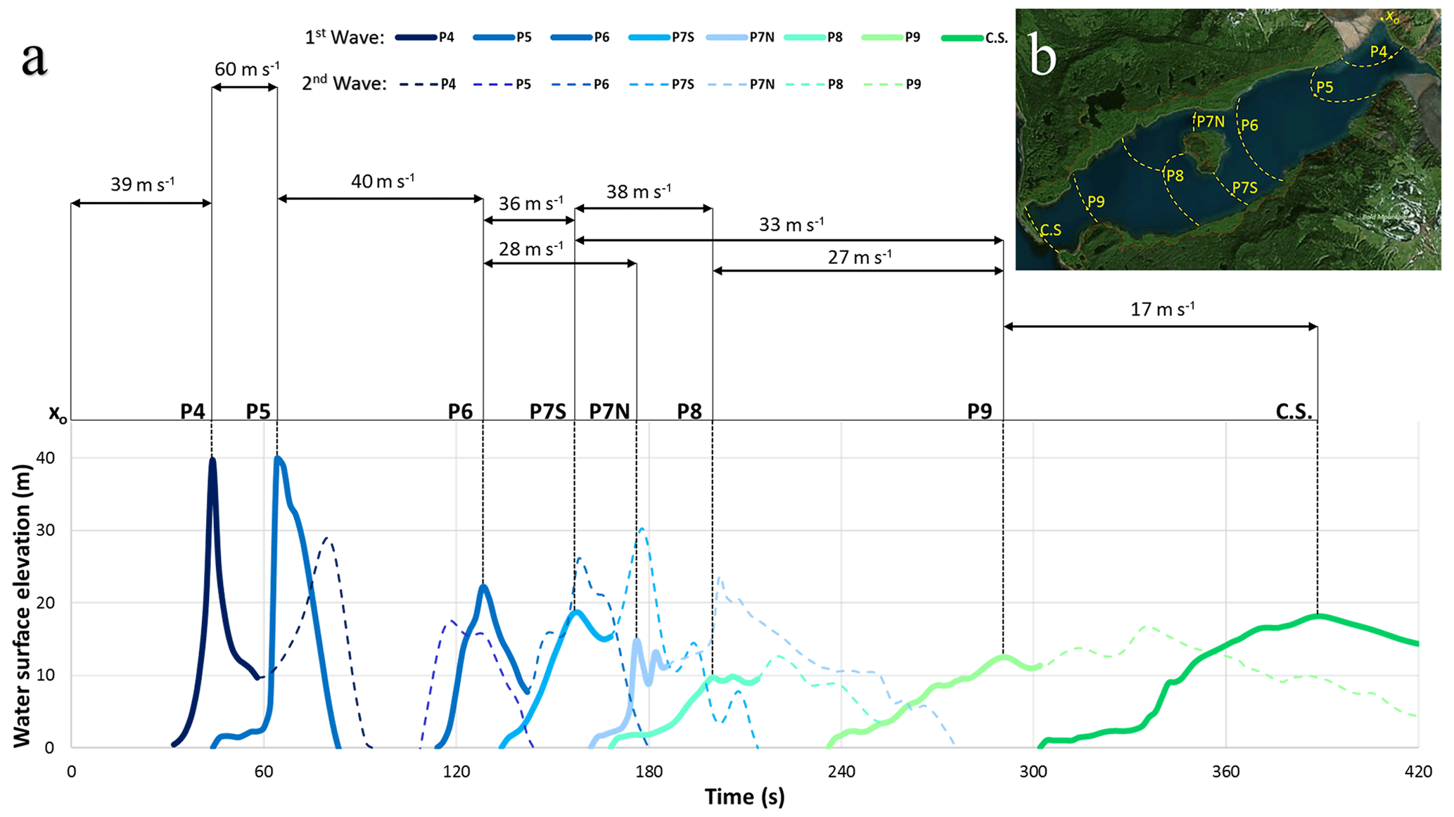
Figure 11(a) The wave attenuation process during its propagation in the bay. The first and the second wave fronts are represented by the full and dashed lines respectively. Mean wave propagation speed is estimated starting from the records at every gauge, considering the position of the first wave front displayed in (b) at the moment of its passage upon the gauges and path lines to estimate the distance of propagation (background topography from © Google Earth Pro 7.3.2.5776; last access: 24 April 2020).
Independently from the grid resolution, general discrepancies in the trimline definition are observed (Fig. 12a, b). Some results are underestimated, as is the case, for example, on the slopes on the southern side of the bay head, the western part of Crillon Inlet, and the Mudslide Creek location. Others are overestimated, such as at the Cascade glacier location, the second highest run-up after the Mudslide Creek, and southern part of Cenotaph Island.
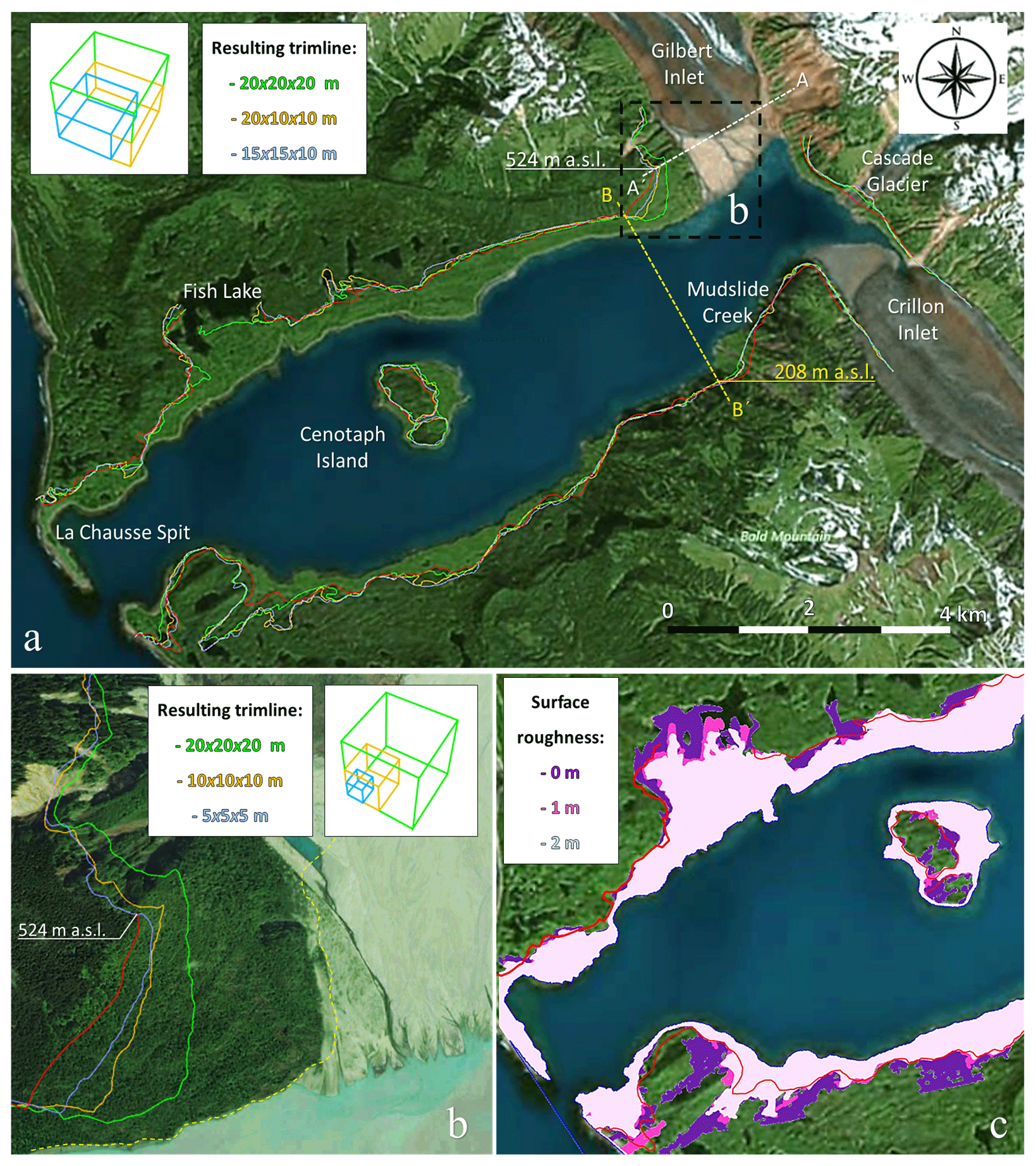
Figure 12(a) Different results of the inundated area and the related trimline, with respect to the observed data (red line), for different grid resolutions and relative roughness equal to 0 m. Sections are reported in Fig. 13. (b) At Gilbert Inlet, the resulting trimlines are defined from the grid resolutions used for the impact area simulations (20, 10, 5 m) and relative roughness is equal to 0 m. The dashed yellow line represents the shoreline before the tsunami event. (c) The resulting inundation area varies depending on the selected relative roughness of 0, 1, or 2 m for the topographic surface (background topography from © Google Earth Pro 7.3.2.5776; last access: 24 April 2020).
The adoption of different values of relative roughness for the topographic surface (0, 1, 2 m, Fig. 12c) results in an evident change for the inundation process. As shown in Fig. 12c, important differences in the flooded area are evident on flatter locations, mainly present in the western region of the bay. Additionally, adopting a roughness of 2 m, the second maximum run-up at the Mudslide Creek results in 210 m a.s.l. Therefore, the trimline obtained from the simulation, with 2 m of relative roughness for a grid resolution of 15 m × 15 m × 10 m, is very close to the one observed, even if some small underestimations and overestimations are still present. However, it is noticed that the simulation with a uniform grid resolution of 20 m can also reproduce the tsunami trimline well.
The fluid mixture process and the submerged propagation of the denser fluid along the bay floor takes place using the second-order approach for the density evaluation. At the end of the simulation, the denser fluid reaches a distance up to 4 km from the impact point, still propagating with a low speed of 5 m s−1 and a thickness of about 35 m. The bulk slide density of the denser fluid decreases during the propagation from 1620 kg m−3 to approximately 1080 kg m−3, which is close to the seawater density.
To accurately simulate landslide-generated impulse wave dynamics in lakes (or fjords) and inundation processes, a high-quality and detailed reconstruction of the pre-event bay configuration is required, especially in areas where the wave characteristics (such as height and speed) change rapidly (as in the impact area). No high-resolution bathymetry and topography pre- and post-1958 event are available for Lituya Bay. The use of the most recent DTM, together with data and information provided by several sources for the case study area, as well as the bay bathymetry before and after the event, allow a reliable reconstruction of the bay configuration previous to the event. This has a high influence on the model performance.
The use of virtual walls and their effects was firstly investigated in the model concept analyses before being considered in the simulations with the topographic surface (Sect. 4.1 and 4.2). The absence of the walls allows the fluid volume to expand during the movement process, while the presence of the walls constricts the fluid until the impact into the sea. This influences the wave characteristics close to the impact location during the propagation phase and the run-up on the opposite slope.
In the simulations with the topographic surface, the topography performs as a normal constriction for the dense fluid at the southeastern boundary of the scar area (Fig. 7). While on the northwestern border the presence of the wall has been adopted as a simple solution to compensate for the lack of topographic elements due to the presence of scars related to secondary rockslides that are not involved in the wave generation (Fig. 2a). Given that almost all of the main rockslide volume impacts the waterbody and generates the impulse wave, the presence of the virtual wall allows the whole denser fluid volume to enter into the waterbody. Otherwise, it would disperse and impact on the glacier, resulting in a wave amplitude and run-up that are too low.
Uniform and non-uniform computational meshes with different grid resolutions have been used to simulate the wave formation and propagation. For the impact area, uniform mesh blocks are set with resolutions of 20, 10, and 5 m. For the whole bay, uniform and non-uniform resolutions such as 20 m × 20 m × 20 m, 20 m × 20 m × 10 m, and 15 m × 15 m × 10 m are used. As expected, the outputs vary according to the resolution of the simulations. Higher accuracy for finer meshes, due to the computational process and the generated computational surface (e.g. roughness), results in a more accurate representation of the natural bathymetry and topography.
In the impact area, it appears that the denser fluid and flow characteristics, using a uniform grid resolution of 20 m, result in lower values with respect to those obtained with a grid resolution of 5 m, except for the flow speed at x0=1342 m and the thickness of the denser fluid (graphs in Fig. 8a).
Concerning the wave propagation (water surface elevation and flow speed; see the graphs in Fig. 10), it is noticed that a grid resolution of 20 m × 20 m × 10 m roughly approximates the results using a grid resolution of 15 m × 15 m × 10 m. Adopting a resolution of 20 m × 20 m × 20 m results mostly in an underestimation of the wave characteristics, where a delay of up to 12 s compared to the other trends is observed.
In order to verify the improvements in the accuracy of the results for finer mesh resolutions, a verification of difference reduction in flow characteristics values is provided for every refinement. The percentage difference and root-mean-square error (RMSE), starting for the series of data recorded from the gauges, are thus estimated. The finest used mesh (15 m × 15 m × 10 m) is taken as a standard. Concerning the water surface elevation, the estimate shows an improvement of the accuracy of the resulting data, with a percentage difference of (RMSE of 4.83 m) and (RMSE of 2.25 m) from the uniform resolutions of 20 m and non-uniform of 20 m × 20 m × 10 m, respectively. An improvement of the accuracy of the flow speed with a percentage difference of (RMSE of 2.02 m s−1) and (RMSE of 1.07 m s−1) from the resolutions of 20 m and 20 m × 20 m × 10 m is also noticed. This comparison of the computational results covers water surface elevations and velocities not only for the local maxima but also during the entire simulation period. This means that small temporal delays in wave propagation already lead to distinctive statistical parameters when comparing two simulations with nearly identical maxima of amplitude and flow velocities to each other.
The examination of the convergence with regard to the mesh size of the numerical model for determining the ordered accuracy can be challenging. Due to the 3D structure of the domain on a natural topographic surface in this study case, a convergence test would not give much more information on the quality of the applied model setup and the results. In a CFD model with a 3D perspective several factors (as observed in the model concept analysis), and not the mesh size alone, can have an important influence on the results, even more so where natural topography and bathymetry for the solid bodies are adopted. It must be said that limitations in computational power and available memory of the computational machine represent an important issue for grid refinement, sometimes leading to the impossibility of achieving the required convergence.
Moreover, the choice of parameters to verify spatial convergence is difficult. If run-up values are highly influenced by the topographic surface, the free water surface or the maximum wave amplitude can be used to verify convergence. Adopting the Richardson extrapolation method (Schwer, 2008), the value of the maximum wave amplitude in the impact area for a grid refinement of 2.5 m is estimated. To reach the spatial convergence, the same value of 208 m a.s.l. is required, thus demonstrating that the results obtained with a uniform mesh size of 5 m are very close to the asymptotic region (interval of confidence). Additionally, Li et al. (2019) state that the resulting wave parameters are mostly dependent on the mesh size in the near field (close to the slide impact) and less dependent on the far field.
The influence of different grid resolutions on the outputs can be clearly observed in the estimated run-up (cross sections in Fig. 13). Adopting the second-order approach for the density evaluation, the maximum run-up in the impact area results in 390, 450, and 524 m a.s.l. for a uniform grid resolution, respectively, of 20, 10, and 5 m (Fig. 13a). The second highest run-up at Mudslide Creek results in 209, 220, and 233 m a.s.l. for a grid resolution of 20 m × 20 m × 20 m, 20 m × 20 m × 10 m, and 15 m × 15 m × 10 m, respectively (Fig. 13b). The present divergence with mesh refinement for the run-up values in the two different locations is explained considering the 3D effect of the topography and the direction of the wave approaching the inland and flowing upon the topographic surface (from the front in the case of section A–A′ and from the side in the case of section B–B′ ).
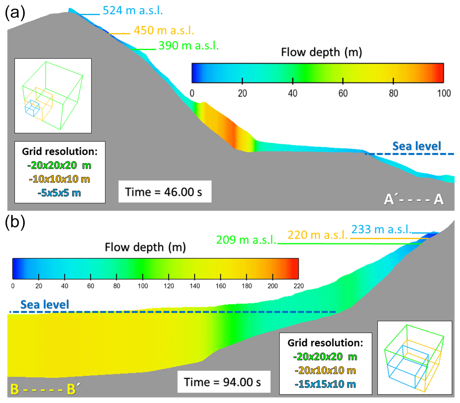
Figure 13Maximum wave run-up resulting from different grid resolutions (see the cross section in Fig. 12). (a) In the impact area the maximum resulting run-up of 524 m a.s.l. relates to the 5 m uniform mesh size. (b) The maximum wave run-up results in 233 m a.s.l. for a non-uniform mesh size of 15 m × 15 m × 10 m at Mudslide Creek (observed run-up was 208 m a.s.l.).
Discrepancies in the resulting trimline with respect to the observed one (Fig. 12) can be related to different sources: (a) to computation error propagation; (b) to the impossibility of sufficiently reducing the grid resolution given the required computational power and memory; (c) to errors in the reconstruction of the bathymetry, the topography, and the shoreline in some areas of the bay, and thus to a not adequate seawater volume to generate the wave; and (d) to the adoption of a smooth surface (zero relative roughness) for the topography surface.
Some instabilities occurred during the calculation for the finer meshes. These are noticed as being mostly caused by isolated fluid drops as the result of free surface breakup (persistent fraction packing locations due to high splashing or foaming; Vanneste, 2012). To avoid instabilities, the default CFPK (fraction packing coefficient) has been reduced by a factor of 10 in the advanced numeric option in Flow-3D.
The estimated trimline for the coarsest resolution used (uniform cell size is 20 m), results in an evident underestimation at Gilbert Inlet but, on the contrary, appears to be quite close to the observed one along the whole bay. An intermediate grid resolution (uniform cell size is 10 m in the impact area, and non-uniform cell size is 20 m × 20 m × 10 m for the whole bay) still gives an underestimated trimline at Gilbert Inlet and results in a slight overestimation along the whole bay. The finest grid resolution used (uniform cell size is 5 m in the impact area, and non-uniform cell size is 15 m × 15 m × 10 m for the whole bay) results in a more accurate trimline, though some underestimations and overestimations are still obvious. The adoption of a relative roughness higher than 1 m avoids some of these overestimations, bringing the resulting trimline closer to the observed one. Additionally, it is observed that a value of roughness higher than 0 m avoids the splashing of water on the topographic surface, allowing an easier definition of the inundated area and a shorter simulation duration.
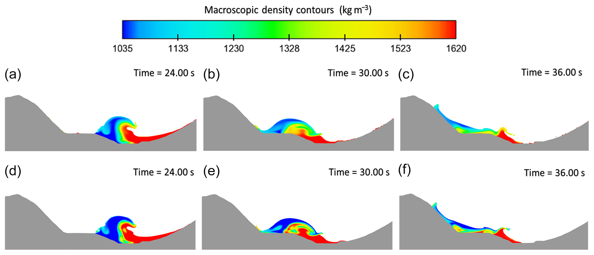
Figure 14Vertical section, for a uniform grid resolution of 5 m, at Gilbert Inlet showing the interaction and the mixing process between the two fluids adopting the first-order approach (a, b, c) and the second-order approach (d, e, f) for the density evaluation.
Concerning grids and the limits with regard to the computation times, the resolution of 15 m × 15 m × 10 m leads to the maximum manageable number of cells for this model (total cells: 50 458 234; active fluid cells: 7 254 191; solid sub-domain cell: 835 184). A resolution of 10 m × 10 m × 10 m has also been tested (active fluid cells: 16 176 884). Despite the use of a more powerful machine (and a parallel license tokens using 32 cores), the simulation could not be completed within a couple of weeks. This could be due to high instability in the model, possibly related to splashing (a reduced value of CFPK did not avoid instabilities in this model).
Note that the mixing process between the two fluids strongly depends on the order approach for density evaluation. As shown in Fig. 14a, b, and c, the first-order approach allows the fluids to mix quickly immediately after the impact, during the air cavity collapse and the run-up. With the second-order approach (Fig. 14d, e, f), the separation of the fluids is much more remarkable. The use of specific order affects the slide material behaviour during its run-out process, where the first-order approach leads to a larger dispersion of the denser fluid inside the seawater.
The described mixing process in Sect. 4.3 is not representative for the Lituya Bay rockslide underwater run-out, since the denser fluid model is adopted at the Gilbert Inlet to recreate the sliding body. Regarding the material deposited in the bay after the tsunami event, and considering the available information provided by literature (Sect. 3.1), it is plausible to consider that the disintegrated rockslide mass did not totally infill the bay floor. The contributions of the material generated from the delta displacements, the sediment released by the glacier, and the eroded soil from the inland are have to be considered as well.
In this study, the 1958 Lituya Bay tsunami event was reproduced. With respect to previous works, we provide an improvement over these by reproducing the physical scale test of Fritz et al. (2001), recreating the bay configuration pre-event, and adopting a specified dataset provided by literature. From the numerical modelling perspective, while most of the previous simulations were set up in 2D, we adopted a 3D numerical modelling approach implemented in Flow-3D to recreate the wave dynamics in the whole bay. In this way, we expanded existing knowledge on this complex physical phenomenon regarding the wave formation and propagation and the 3D effects on the wave characteristics due to the interaction with the recreated bay surface.
Our results attest that a good model can represent what actually happened during the entire event and give a better understanding of the Lituya Bay tsunami event on 9 July 1958. The impact area and the whole inundated bay have to be analysed separately to get more details of the entire process.
The reconstruction (or definition) of a realistic, reliable, and detailed bathymetry and topography is recommended for an impulse wave simulation since the surface generated by the computation grid influences the definition of the inundated area during wave propagation and inundation. Having reliable bathymetry data and realistic depth and shape information of the bay floor before the event enables the simulation of a reliable interaction between the impulse wave and the bay floor in order to, for example, observe the wave behaviour during its propagation (breaking process or maintaining its shape and characteristics).
A detailed topography allows for simulating a trimline that is as similar as possible to the observed one. This is depending on the surface generated by the computation grid and its spatial resolution. A high grid resolution can highlight topography details that can be fundamental to estimating the flooded area. The definition of the pre-event shoreline is relevant, mostly where it has been extremely modified by the tsunami event. This happens principally in the impact area, where the rockslide entered into the waterbody and the tsunami featured highest intensities (in terms of speed and water height). In general, this highlights the need for adequate pre-event information of the terrain, especially in regions with lower water depths and that impact with the surrounding ground.
The following main conclusions are reported.
-
The model concept analysis reliably reflects results from experiments and numerical simulations proposed by Fritz et al. (2001) and Basu et al. (2010), despite an overestimation of the run-up values. It is observed that a denser fluid is a suitable, simple concept to recreate the impact of a sliding mass in a waterbody, in this case with an impact speed of about 92–114 m s−1 (for a slope inclination of 35∘, Fig. 6c). For this concept, the consideration of the bulk slide volume and density is adequate for the reproduction of the impact intensity. The presence of Gilbert glacier and virtual walls to constrain the slide material during the collapse process has a crucial influence on wave formation and run-up.
-
It is demonstrated that the rockslide represents the main trigger for the impulse wave generation in Lituya Bay (as proposed by Fritz et al., 2009), and for the forest destruction. The simulated fluid impact into the waterbody reproduces the wave dynamics and run-up at Gilbert Inlet. It also represents the primary trigger for the wave propagation along the whole bay, including water surface elevation, wave propagation speed, inundation effects, and trimline definition. On the other side, it can be confirmed that the rockslide material alone does not explain the total infill of the bay bed after the 1958 tsunami event.
-
The resulting maximum wave amplitude of 208 m and the maximum run-up of 524 m a.s.l. are obtained using a uniform mesh size of 5 m. Even though the simulation shows the wave overtopping the hill facing the slide source, then flowing diagonally downslope, the simulations still significantly underestimate the observed trimline.
-
A mesh size of 15 m × 15 m × 10 m is required for a reliable simulation of the wave dynamics propagation along the whole bay. The estimated trimline fits best to the observed one when a relative roughness of 2 m is set for the vegetated part of the topographic surface. The inundation is not only caused by the primary wave but also by several secondary reflected waves. It is observed that the wave reacts to the bathymetry and topography shape, varying its features during the propagation and evolving from a high-speed, steep-front wave at the head of the bay, to a slow-speed, long-period wave when approaching the seaside.
-
The use of different order approaches for the density evaluation has been tested, resulting in different behaviour for the mixing process between the two fluids, occurring faster for the first-order approach. No important influences on the wave amplitudes and run-up heights are observed.
-
The relative difference and the RMSE for the water surface elevation and flow speed values highlight the improvement in accuracy when adopting a finer mesh. In general, this work supports the necessity of using a grid resolution that is as high as possible to ensure a reliable model and obtain accurate outputs and insights into the wave dynamics.
-
The results confirm that the bay configuration before the tsunami event has been reconstructed well and confirm the descriptions provided by Miller (1960). The possibility of having available bathymetry and topography data before and after a tsunami event makes the interpretation and reconstruction of the case study easier and more precise. The lack of data and limited information concerning the 1958 Lituya Bay tsunami event obligates experts to give their own subjective interpretation.
Following these remarks and what has been discussed in Sect. 5, some considerations in terms of computational effort vs. trimline reliability are proposed. Utilising the same computational resource (see Sect. 3.2.1), the wave propagation model with a uniform grid resolution of 20 m already gives a trimline quite close to the observed one with a calculation time of 3 h. When adopting a finer resolution of 15 m × 15 m × 10 m, even if the trimline results are more accurate, overestimations are still noticed. The calculation takes almost 7 d to run. This high computational time can be still considered an affordable one for numerical model simulations. Despite this, in an application for hazard analysis, a model with a coarser resolution can represent a fast and sufficient solution for a rough assessment of a landslide-generated impulse wave event, where it is possible to already obtain a good approximation of the inundated area. Regardless, to get more details and insights into the wave dynamics, models with a finer mesh are recommended, where different scenarios adopting different values for the topographic surface roughness have to be tested.
The use of a more powerful computational machine would allow for the adoption of a mesh size as fine as is required to reach the convergence. Applying a convergence test on standardised models with an artificial geometry would lead to a better understanding of the influence of the mesh size on wave parameters and the run-up heights.
In conclusion, Flow-3D represents a suitable tool for landslide-generated impulse wave simulations. The software can provide a good approximation for the impact process with the limitations of the chosen modelling concept regarding the representation of the physics of the impact process. Future works will focus on the use of different models (as the granular flow or the solid body) to reproduce the sliding process. Some discrepancies in the inundation dynamics and the trimline estimation still occur in the model. This can be explained by the software limits, computational errors, and imprecision in the bay reconstruction due to a lack of information. It has to be said that observation data are also not always perfectly represented everywhere.
With regard to the last research questions concerning the application of this 3D numerical approach and its capabilities (Sect. 1), this work shows the value and applicability of models like this not only for back-calculating and recreating past events but for risk assessment in fjords and mountain lakes potentially endangered by large impacts from the slopes. The shape of the Lituya Bay, as a narrow and long fjord, and the gravitational process that generated the impulse wave (a rockslide evolved in a rock avalanche) represent a situation that can also be found in other mountain regions like the Alps.
The simulation video and additional data (model code, reconstructed bathymetry, and topography stored as a .stl file) that support the findings of this study are available from the following repository: https://doi.org/10.5281/zenodo.3831448 (Franco, 2020).
The original DTM data are available from the DGGS Elevation Portal (DGGS, 2020), the bathymetry data from the National Ocean Service: Hydrographic Surveys with Digital Sounding (Survey IDs: H08492, 1959; H04608, 1926).
AF designed the case study and the main research goals, with support from BG concerning the modelling in Flow-3D. AF prepared the manuscript with contributions of JM, BSM, MS, and BG. All authors discussed, reviewed, and edited the different versions of the manuscript.
The authors declare that they have no conflict of interest.
This article is part of the special issue “Advances in computational modelling of natural hazards and geohazards”. It is a result of the following conference: Geoprocesses, geohazards – CSDMS 2018, Boulder, USA, 22–24 May 2018.
Thanks are owed to the NHESS Editor and the (anonymous) reviewers, whose comments and remarks greatly improved the model setup, the quality of the achieved results, clarity, and finally the quality of this paper. Thanks are further owed to Markus Grünzner (Flow Science Germany) for his great and quick support in improving the model setup.
This paper was edited by Randall LeVeque and reviewed by Carl B. Harbitz and one anonymous referee.
This research is funded by the University of Innsbruck in support of the doctoral programme “Natural Hazards in Mountain Regions” (https://www.uibk.ac.at/alpinerraum/dps/dp-mountainhazards/, last access: 12 June 2020). It is related to the research project “Wave formation, propagation and run-up in natural mountain lakes from a cascade hazard perspective – analysis and modelling of triggering processes, lake's morpho-dynamics and potential downstream hazard effects”.
Basu, D., Das, K., Green, S., Janetzke, R., and Stamatakos, J.: Numerical simulation of surface waves generated by subaerial landslide at Lituya Bay Alaska, J. Offshore Mech. Arct., 132, 041101, https://doi.org/10.1115/1.4001442, 2010.
Braathen, A., Blikra, L. H., Berg, S. S., and Karlsen, F.: Rock-slope failures in Norway: type, geometry, deformation mechanisms and stability, Norsk Geol. Tidsskr., 84, 67–88, 2004.
Bridge, T.: When mountains fall into the sea: https://www.hakaimagazine.com/, last access: September 2018.
Chuanqi, S., Yi, A., Qiang, W., Qingquan, L., and Zhixian, C.: Numerical simulation of landslide-generated waves using a soil-water coupling smoothed particle hydrodynamics model, Adv. Water Resour., 92, 130–141, https://doi.org/10.1016/j.advwatres.2016.04.002, 2016.
Das, K., Janetzke, R., Basu, D., Green, S., and Stamatakos, J.: Numerical Simulations of Tsunami Wave Generation by Submarine and Aerial Landslides Using RANS and SPH Models, 28th International Conference on Ocean, Offshore and Arctic Engineering, Honolulu, USA, 5, 581–594, https://doi.org/10.1115/OMAE2009-79596, 2009.
DGGS: DGGS Elevation portal – Alaska Division of Geological and Geophysical Surveys, https://elevation.alaska.gov/#65.14611:-155.74219:4, last access 24 March 2020.
Evers, F. M., Heller, V., Fuchs, H., Hager, W. H., and Boes, R. M.: Landslide generated impulse waves in reservoirs – Basics and computation, VAW Communications, Laboratory of Hydraulics, Hydrology and Glaciology (VAW), ETH Zurich, Zurich, Switzerland, 254 pp., 2019.
Flow Science Inc.: Flow-3D®, Version 12.0, User's Manual, https://www.flow3d.com (last access: 31 January 2020), Santa Fe, USA, 2018.
Franco, A.: Lituya Bay 1958 Tsunami – pre-event bathymetry reconstruction and 3D-numerical modelling utilizing the CFD software Flow-3D, Zenodo, https://doi.org/10.5281/zenodo.3831448, 2020.
Fritz, H. M., Hager, W. H., and Minor, H. E.: Lituya Bay case: Rockslide impact and wave run-up, Sci. Tsunami Hazards, 19, 3–22, 2001.
Fritz, H. M., Mohammed, F., and Yoo, J.: Lituya Bay landslide impact generated mega-tsunami 50th anniversary, Pure Appl. Geophys., 166, 153–175, https://doi.org/10.1007/s00024-008-0435-4, 2009.
Furseth, A.: Dommedagsfjellet - Tafjord 1934, Gyldendal Norsk Forlag A/S, Oslo, Norway, 1958.
Gauthier, D., Anderson, S. A., Fritz, H. M., and Giachetti, T.: Karrat Fjord (Greenland) Tsunamigenic landslide of 17 June 2017: initial 3D observations, Landslides, 15, 327–332, https://doi.org/10.1007/s10346-017-0926-4, 2017.
González-Vida, J. M., Macías, J., Castro, M. J., Sánchez-Linares, C., de la Asunción, M., Ortega-Acosta, S., and Arcas, D.: The Lituya Bay landslide-generated mega-tsunami – numerical simulation and sensitivity analysis, Nat. Hazards Earth Syst. Sci., 19, 369–388, https://doi.org/10.5194/nhess-19-369-2019, 2019.
Haeussler, P. J., Gulick, S. P. S., McCall, N., Walton, M., Reece, R., Larsen, C., Shugar, D. H., Geertsema, M., Venditti, J. G., and Labay, K.: Submarine deposition of a subaerial landslide in Taan Fjord, Alaska, J. Geophys. Res.-Earth, 123, 2443–2463, https://doi.org/10.1029/2018JF004608, 2018.
Harbitz, C., Pedersen, G., and Gjevik, B.: Numerical simulations of large water waves due to landslides, J. Hydraul. Eng. 119, 1325–1342, 1993.
Hall Jr., J. V. and Watts, G. M.: Laboratory investigation of the vertical rise of solitary waves on impermeable slopes, U.S. Army Corps of Engineers, Beach Erosion Board, 173–189, 1953.
Harlow, F. H. and Welch, J. E.: Numerical Calculation of Time-Dependent Viscous Incompressible Flow, Phys. Fluids, 8, 2182–2189, https://doi.org/10.1063/1.1761178, 1965.
Heller, V., Hager, W. H., and Minor, H.-E.: Landslide generated impulse waves in reservoirs – Basics and computation, VAW Communications, 211, Laboratory of Hydraulics, Hydrology and Glaciology (VAW), ETH Zurich, Zurich, Switzerland, 211 pp., 2009.
Heller, V. and Hager, W. H.: Impulse product parameter in landslide generated impulse waves, J. Waterw. Port Coast., 136, 145–155, https://doi.org/10.1061/(ASCE)WW.1943-5460.0000037, 2010.
Hinze, J. O.: Turbulence, McGraw-Hill, New York, USA, 1975.
Hirt, C.W. and Nichols, B. D.: Volume of Fluid (VOF) Method for the Dynamics of Free Boundaries, J. Comput. Phys., 39, 201–225, https://doi.org/10.1016/0021-9991(81)90145-5, 1981.
Hirt, C.W. and Sicilian, J.M.: A Porosity Technique for the Definition of Obstacles in Rectangular Cell Meshes, Proceedings of the Fourth International Conference on Ship Hydrodynamics, National Academy of Sciences, Washington, D.C., USA, 25–27 September 1985, 1–19, 1985.
Holmsen, G.: De siste bergskred i Tafjord og Loen, Norge, Svensk geografisk Arbok 1936, Lunds Universitet, Geografiska Institutionen Meddelande, 124, 171–190, 1936.
Huber, A. and Hager, W. H.: Forecasting impulse waves in reservoirs, Dix-neuvième Congrès des Grands Barrages C31, Florence, Italy, Commission International des Grands Barrages, Paris, France, 993–1005, 1997.
Kamphuis, J. W. and Bowering, R. J.: Impulse waves generated by landslides, Coast. Eng., 35, 575–588, https://doi.org/10.9753/icce.v12.35, 1970.
Körner H. J.: Reichweite und Geschwindigkeit von Bergstürzen und Fliessschneelawinen, Rock Mech., 8, 225–256, 1976.
Li, G., Chen, G., Li, P., and Jing, H.: Efficient and Accurate 3-D Numerical Modelling of Landslide Tsunami, Water, 11, 2033, https://doi.org/10.3390/w11102033, 2019.
Mader, C. L.: Modelling the 1958 Lituya Bay mega-tsunami, Sci. Tsunami Hazards, 17, 57–67, 2001.
Mader C. L and Gittings M. L.: Modelling the 1958 Lituya Bay mega-tsunami II, Sci. Tsunami Hazards, 20, 241–250, 2002.
Mao J., Zhao L., Liu X., Cheng J., and Avital E.: A three-phases model for the simulation of landslide-generated waves using the improved conservative level set method, Comput. Fluids, 159, 243–253, ISSN: 0045-7930, https://doi.org/10.1016/j.compfluid.2017.10.007, 2017.
Miller, D.: Giant Waves in Lituya Bay, Alaska: A Timely Account of the Nature and Possible Causes of Certain Giant Waves, with Eyewitness Reports of Their Destructive Capacity, professional paper, US Government Printing Office, Washington, D.C., USA, 49–85, 1960.
Noda, E.: Water waves generated by landslides, J. Waterway Div-ASCE., 96, 835–855, 1970.
Pastor, M., Herreros, I., Fernndez Merodo, J. A., Mira, P., Haddad, B., Quecedo, M., González, E., Alvarez-Cedrón, C., and Drempetic, V.: Modelling of fast catastrophic landslides and impulse waves induced by them in fjords, lakes and reservoirs, Eng. Geol., 109, 124–134, https://doi.org/10.1016/j.enggeo.2008.10.006, 2008.
Paronuzzi, P. and Bolla, A.: The prehistoric Vajont rockslide: an update geological model, Geomorphology, 169–170, 165–191, https://doi.org/10.1016/j.geomorph.2012.04.021, 2012.
Pararas-Carayannis, G.: Analysis of mechanism of tsunami generation in Lituya Bay, Sci. Tsunami Hazards, 17, 193–206, 1999.
Quecedo, M., Pastor, M., and Herreros, M.: Numerical modelling of impulse wave generated by fast landslides, Int. J. Numer. Meth. Eng., 59, 1633–1656, https://doi.org/10.1002/nme.934, 2004.
Rady, R. M. A. E.: 2D-3D Modeling of Flow Over Sharp-Crested Weirs, J. Appl. Sci. Res., 7, 2495–2505, 2011.
Slingerland, R. L. and Voight, B.: Occurrences, properties, and predictive models of landslide-generated water waves, Developments in Geotechnical Engineering 14B, Rockslides and avalanches 2, Engineering Sites, Elsevier Scientific Publishing, Amsterdam, the Netherlands, 317–397, 1979.
Schwaiger, H. F. and Higman, B.: Lagrangian hydrocode simulations of the 1958 Lituya Bay tsunamigenic rockslide, Geochem. Geophys. Geosyst., 8, Q07006, https://doi.org/10.1029/2007GC001584, 2007.
Schwer L. E.: Is your mesh refined enough? Estimating Discretization Error using GCI, in 7th German LS-DYNA Forum, Bamberg, Germany, 2008.
Sepúlveda, S. A., A. Serey, M. Lara, A. Pavez, and Sepúlveda, S. A., Serey, A., Lara, M., Pavez, A., Rebolledo, S.: Landslides induced by the April 2007 Aysén Fjord earthquake, Chilean Patagonia, Landslides, 7, 483–492, https://doi.org/10.1007/s10346-010-0203-2, 2010.
Sharpe, C.: Landslides and Related Phenomena, Columbia Univ. Press, New York, USA, 1938.
Synolakis, C.: The runup of solitary waves, J. Fluid. Mech., 185, 523–545, https://doi.org/10.1017/S002211208700329X, 1987.
Tocher, D. and Miller D. J.: Field observations on effects of Alaska earthquake of 10 July, 1958, Science, 129, 3346, 394–395, https://doi.org/10.1126/science.129.3346.394, 1959.
Tognacca, C.: Beitrag zur Untersuchung der Entstehungsmechanismen von Murgangen, VAW communications, 164, Laboratory of Hydraulics, Hydrology and Glaciology, ETH Zurich, Zurich, Switzerland, 1999.
US Coast and Geodesic Survey: Survey id: H04608: NOS Hydrographic Survey, 1926-12-31, available at: https://data.world/us-noaa-gov/f6786b28-ea06-4c9a-ac30-53cb5356650c (last access: 28 September 2018), 1926.
US Coast and Geodesic Survey: Survey id: H08492: NOS Hydrographic Survey, Lituya Bay, Alaska, 1959-08-27, available at: https://data.world/us-noaa-gov/9401821a-28f5-4846-88db-43e702a5b12b (last access: 28 September 2018), 1959.
U.S. Coast and Geodetic Survey: Chart 8505, Lituya Bay, Washington D.C., USA, 1942.
U.S. Coast and Geodetic Survey: Chart 8505, Lituya Bay, Washington D.C., USA, 1969.
U.S. Coast and Geodetic Survey: Chart 16762, Lituya Bay, Washington D.C., USA, 1990.
Vanneste, D.: Experimental and numerical study of wave-induced porous flow in rubble-mound breakwaters, Ph.D. thesis, Gent University, Gent, Belgium, 2012.
Varnes, D.: Landslide type and Processes, In Landslides and Engineering Practice, H R B Special Rep., 29, 22–47, National Research Council (US), Washington D.C., USA, 1958.
Vasquez, J. A.: Modelling the generation and propagation of landslide-generated landslide, CSCE SCGC, Leadership in Sustainable Infrastructure, Annual Conference, May 31–June 3 2017, Vancouver, Canada, 2017.
Yakhot, V. and Smith, L. M.: The Renormalization Group, the e-Expansion and Derivation of Turbulence Models, J. Sci. Comput., 7, 35–61, https://doi.org/10.1093/gji/ggv026, 1992.
Wang, J., Ward, S. N., and Xiao, L.: Numerical simulation of the December 4, 2007 landslide-generated tsunami in Chehalis Lake, Canada, Geophys. J. Int., 201, 372–376, https://doi.org/10.1093/gji/ggv026, 2015.
Ward, S. N. and Day, S.: The 1958 Lituya bay landslide and tsunami – A tsunami ball approach, J. Earthq. Tsunami, 4, 285–319, https://doi.org/10.1142/S1793431110000893, 2010.
Weiss, R. and Wuennemann, K.: Understanding tsunami by landslides as the next challenge for hazard, risk and mitigation: Insight from multi-material hydrocode modeling, American Geophysical Union, Fall Meeting 2007, San Francisco, CA, USA, S51C-06, 2007.
Weiss, R., Fritz, H. M., and Wünnemann, K.: Hybrid modeling of the mega-tsunami runup in Lituya Bay after half a century, Geophys. Res. Lett., 36, L09602, https://doi.org/10.1029/2009GL037814, 2009.
Welch, J. E., Harlow, F. H., Shannon, J. P., and Daly, B. J.: The MAC Method: A Computing Technique for Solving Viscous, Incompressible, Transient Fluid Flow Problems Involving Free-surfaces, Los Alamos Scientific Laboratory report LA-3425, Los Alamos, NM, USA, 1966.
Wiegel, R. L.: Oceanographical Engineering, Prentice Hall, Englewood Cliffs, USA, 1964.
Xenakis, A. M., Lind, S. J., Stansby, P. K., and Rogers, B. D.: Landslides and tsunamis predicted by incompressible smoothed particle hydrodynamics (SPH) with application to the 1958 Lituya Bay event and idealized experiment, P. R. Soc. A, 473, 1–18, https://doi.org/10.1098/rspa.2016.0674, 2017.