Can ocean community production and respiration be determined by measuring high-frequency oxygen profiles from autonomous floats?

Gordon, Christopher; Fennel, Katja; Richards, Clark; Shay, Lynn K.; Brewster, Jodi K.

doi:https://doi.org/10.5194/bg-17-4119-2020

Articles | Volume 17, issue 15

https://doi.org/10.5194/bg-17-4119-2020

Special issue:

Biogeochemistry in the BGC-Argo era: from process studies...

https://doi.org/10.5194/bg-17-4119-2020

Articles | Volume 17, issue 15

Research article

14 Aug 2020

Research article |

| 14 Aug 2020

Can ocean community production and respiration be determined by measuring high-frequency oxygen profiles from autonomous floats?

Christopher Gordon, Katja Fennel, Clark Richards, Lynn K. Shay, and Jodi K. Brewster

Abstract

Oceanic primary production forms the basis of the marine food web and provides a pathway for carbon sequestration. Despite its importance, spatial and temporal variations of primary production are poorly observed, in large part because the traditional measurement techniques are laborious and require the presence of a ship. More efficient methods are emerging that take advantage of miniaturized sensors integrated into autonomous platforms such as gliders and profiling floats. One such method relies on determining the diurnal cycle of dissolved oxygen in the mixed layer and has been applied successfully to measurements from gliders and mixed-layer floats. This study is the first documented attempt to estimate primary production from diurnal oxygen changes measured by Argo-type profiling floats, thus accounting for the whole euphotic zone. We first present a novel method for correcting measurement errors that result from the relatively slow response time of the oxygen optode sensor. This correction relies on an in situ determination of the sensor's effective response time. The method is conceptually straightforward and requires only two minor adjustments in current Argo data transmission protocols: (1) transmission of measurement time stamps and (2) occasional transmission of downcasts in addition to upcasts. Next, we present oxygen profiles collected by 10 profiling floats in the northern Gulf of Mexico, evaluate whether community production and respiration can be detected, and show evidence of internal oscillations influencing the diurnal oxygen signal. Our results show that profiling floats are capable of measuring diurnal oxygen variations although the confounding influence of physical processes does not permit a reliable estimation of biological rates in our dataset. We offer suggestions for recognizing and removing the confounding signals.

Please read the corrigendum first before continuing.

Download & links

Article (PDF, 5432 KB)

Notice on corrigendum
The requested paper has a corresponding corrigendum published. Please read the corrigendum first before downloading the article.
Article (5432 KB)

Corrigendum

Download & links

The requested paper has a corresponding corrigendum published. Please read the corrigendum first before downloading the article.

How to cite

How to cite.

Dates

Received: 02 Apr 2020 – Discussion started: 08 Apr 2020 – Revised: 11 Jun 2020 – Accepted: 06 Jul 2020 – Published: 14 Aug 2020

1 Introduction

Oceanic primary production forms the basis of the oceanic food web and is a major component of the global carbon cycle by providing a pathway for carbon sequestration in the ocean interior. Although primary production is intrinsic to understanding biogeochemical dynamics in the ocean, its temporal and spatial variations are not well observed. Historically, it has been estimated by performing 12 to 24 h bottle incubations using ¹⁴C (Steeman-Nielsen, 1952; Marra, 2009). These incubations require substantial effort and the presence of a ship, while only providing point estimates of production. Satellites estimate production on the global scale but rely on assumptions about the photosynthesis–irradiance relationship, the vertical structure of biomass, and global regressions of observed productivity with sea surface temperature, all with inherent limitations.

Both of the above methods quantify net primary production (NPP), defined as the total rate of photosynthetically fixed carbon minus autotrophic respiration. The total fixation of carbon is referred to as gross primary production (GPP). Other definitions of primary production consider losses by the whole planktonic community including autotrophic and heterotrophic respiration. Community respiration (R) is the total rate of carbon respired by autotrophs and heterotrophs. The balance between GPP and R is referred to as net community production (NCP = GPP −R), where a positive (negative) NCP indicates net production (net respiration). A positive NCP, i.e., net biomass production by the planktonic community, is expressed as an increase in biomass or in exported carbon or a combination of both.

NCP in the mixed layer can be estimated by measuring the ratio of dissolved oxygen to dissolved argon ([O₂]∕[Ar]) (Kaiser et al., 2005; Cassar et al., 2009; Hamme et al., 2012; Tortell et al., 2014). The two gases have similar physical properties with regard to their solubility, but Ar is biologically inactive while oxygen is produced and consumed by production and respiration. The ratio of [O₂]∕[Ar] can thus be used to partition changes in oxygen into physical and biological components, where the biological component represents NCP over the timescale of mixed-layer gas exchange, usually about 10 to 30 d. This technique offers a better time–space resolution than ¹⁴C incubations as it can be applied in high-precision and continuously to a steaming ship's seawater flow through, making it a good candidate for deployment on ships of opportunity, but does require the presence of a ship and is limited to the mixed layer.

The emergence and integration of miniaturized biogeochemical sensors into autonomous platforms have opened new avenues for measuring production. Numerous studies have used particulate beam attenuation (Cullen et al., 1992; Claustre et al., 1999; Kinkade et al., 1999; Gernez et al., 2010; Dall'Olmo et al., 2011; Omand et al., 2017; White et al., 2017) or dissolved oxygen (Caffrey, 2003; Riser and Johnson, 2008; Johnson, 2010; Nicholson et al., 2015; Briggs et al., 2018; Barone et al., 2019) to estimate production from such platforms. Riser and Johnson (2008) measured oxygen profiles with profiling floats every 10 d in the subtropical Pacific Ocean. Oxygen below the mixed layer showed a steady increase throughout the stratified period. The slope of the oxygen buildup allowed estimation of seasonally averaged NCP below the mixed layer. GPP and R have also been estimated from diurnal cycles of oxygen within the mixed layer observed by gliders (Nicholson et al., 2015) and mixed-layer floats (Briggs et al., 2018). A similar approach has been applied to diurnal cycles of beam-c measurements from an underway ship flow through (White et al., 2017). In Nicholson et al. (2015), approximately 14 glider profiles per day were averaged over a study period of 110 d to obtain the average diurnal cycle of dissolved oxygen within the mixed layer. The techniques applied in White et al. (2017) and Briggs et al. (2018) instead used continuous measurements to observe daily cycles. In Briggs et al. (2018), by measuring the decline of dissolved oxygen through the night, the respiration rate R was determined. Then, by measuring the increase in oxygen during the day and subtracting R, GPP was calculated.

These previous studies are encouraging but required large averaging periods or neglected at least some portion of the water column where production is likely to occur (e.g., White et al., 2017; Briggs et al., 2018) or both (Riser and Johnson, 2008; Nicholson et al., 2015). Here, we test whether diurnal cycles of dissolved oxygen can be observed with sufficient accuracy from Argo-type floats to estimate daily productivity for the whole euphotic zone. We use measurements from 10 floats that were deployed in the Gulf of Mexico in 2017 and profiled continuously for several days. This work most directly extends previous research with autonomous floats by Briggs et al. (2018) but, by using profiling rather than mixed-layer floats, explicitly considers the entire euphotic zone. To answer the overarching question of whether GPP, R, and thus NCP can be estimated from continuously profiling floats, two sets of specific questions are addressed. (1) Are the floats capable of sampling at the rate and accuracy required to resolve diurnal-scale changes in oxygen? And (2) what are the primary physical or biological drivers of oxygen change in the upper ocean at our study site? Are there physical processes that can confound the biological signal? If so, can the two signals be separated?

The first set of questions addresses technical aspects of the measurement. It is necessary to determine whether profiling floats are able to properly resolve the diurnal signal. While oxygen optodes have been shown to be reliable and stable when deployed on autonomous floats (Tengberg et al., 2006; Gruber et al., 2010), with only a weak drift of less than 1 % per year (Bushinsky et al., 2016; Bittig and Körtzinger, 2017), they require pressure and salinity (Bittig et al., 2015), in-air gain (Johnson et al., 2015; Nicholson and Feen, 2017), and response time (Bittig et al., 2014, 2018) corrections. While pressure and in-air gain corrections are typically applied, response time correction is not done routinely even though errors can be of the order of 10 mmol m⁻³ in the euphotic zone. The ability to reliably perform these corrections will be paramount to measuring the diurnal oxygen signal.

The second set of research questions addresses the environmental side of measuring production autonomously in situ. The floats were deployed in the dynamic but oligotrophic shelf break region in the northern Gulf of Mexico where primary production is low. Given this, the biological signal is much weaker than during the first demonstration of diurnal oxygen measurement by Briggs et al. (2018) in the North Atlantic Ocean, which was conducted during the spring bloom.

This paper is structured as follows. In Sect. 2.1, float functionality and deployment as well as sensor calibration and data processing are described. The first set of research questions is addressed in Sect. 3, where the mathematical formalism underlying the optode measurement, a method for determining the sensor response time in situ, and an error analysis are presented. The second set of research questions is addressed in Sect. 4, where possible drivers of oxygen variability in the upper ocean are explored, including physical processes that can influence dissolved oxygen in the euphotic zone. Section 5 contains conclusions and recommendations.

2 Methods

2.1 Float functionality and deployment

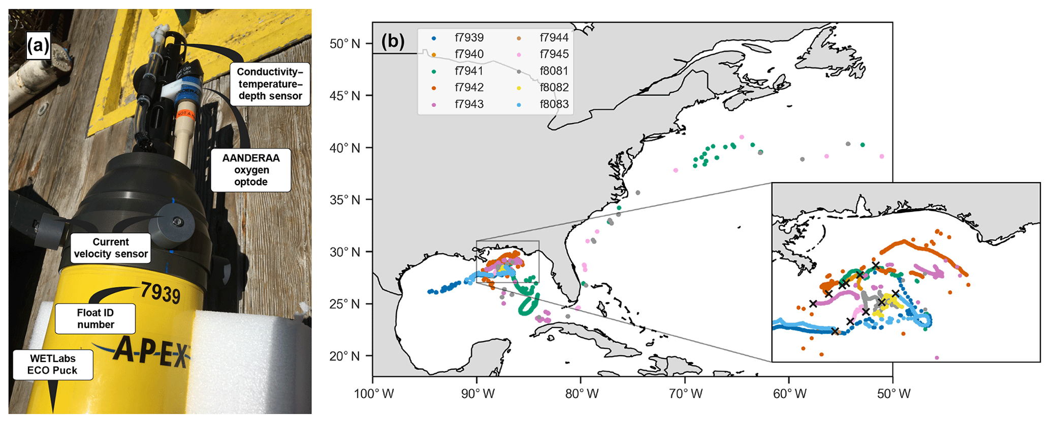
https://bg.copernicus.org/articles/17/4119/2020/bg-17-4119-2020-f01

Figure 1(a) Photo of float f7939 with the sensors labeled. (b) Map of the 10 deployment stations (black crosses in inset) and float trajectories.

In May 2017, 10 autonomous ElectroMagnetic-Autonomous Profiling EXplorer (EM-APEX) floats were deployed in the northern Gulf of Mexico near the Mississippi Delta (Fig. 1, Shay et al., 2019). The floats were equipped with a Sea-Bird Scientific CTD; two electromagnetic current velocity sensors; a WETLabs ECO Puck bio-optical triplet which measures chlorophyll fluorescence, optical backscattering, and colored dissolved organic matter (CDOM) fluorescence; and an Aanderaa 4330 oxygen optode. This study primarily uses data from the oxygen optode and CTD.

The floats operated in two different profiling modes: (1) the traditional “park-and-profile” mode where floats surfaced once every 5 to 10 d and drifted at 1000 m depth in between profiles, and (2) the “continuous” mode where floats profiled the top 1000 m continuously, pausing only to transmit data at the surface following an upcast (this resulted in one profile about every 3 h). The vertical resolution of measurements was about 5 dbar. No depth binning was performed on the sensor data. The profiling mode of the floats was changed via two-way Iridium communication.

The floats were deployed in a grid (Fig. 1b inset), and a set of discrete shipboard measurements was taken in conjunction with most deployments. The floats were initially set to continuous mode for about 1 week. After that, the floats operated in park-and-profile mode until hurricanes Irma and Nate passed through the Gulf of Mexico and the floats were switched back to continuous mode for about 2 weeks. The dataset thus contains three periods of high-frequency sampling (after deployment and during the passage of the two hurricanes). While none of the floats was located directly within the path of the hurricanes, most of them experienced a sea state affected by high winds.

Three floats failed less than 1 month into the deployment (see Table 1). Location data suggest that during continuous-mode sampling these floats drifted near or onto shelf areas with low-density surface waters for which they were not properly ballasted. Without the required buoyancy to surface, the floats would have been trapped below the surface. One of the other floats also encountered a low-salinity plume and was not surfacing and transmitting for an extended period of time but resumed functioning normally again later. Two floats transmitted data until the end of 2017, and the remaining five floats operated until early 2019, with the last transmission occurring on 6 March 2019. Three floats were entrained into the Loop Current and left the Gulf of Mexico, eventually ending up in the North Atlantic (Fig. 1b). In total, the 10-float fleet measured over 2700 profiles – over 1600 of these during continuous-mode sampling.

2.2 Sensor calibration and data processing

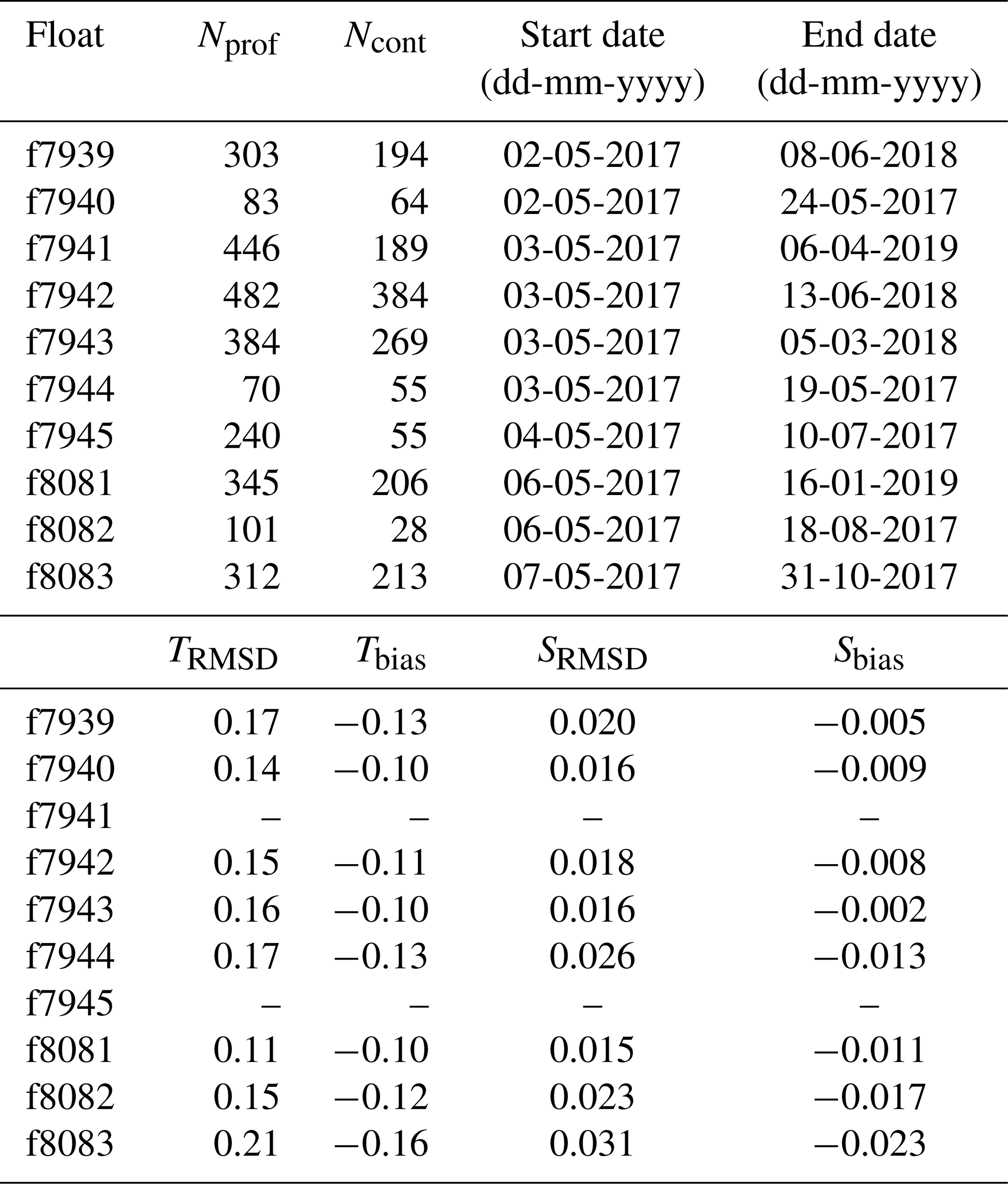
At most deployment stations, a CTD cast to 2000 m, or to the bottom if shallower, was performed using a Sea-Bird SBE 9 CTD for comparison between ship measurements and the first profile recorded by each float. For two floats, the CTD cast was not carried out because of rough seas. The CTD and float profiles agree within an average root-mean-square difference (RMSD) of 0.16 ^∘C and 0.02 (N=8) for temperature and salinity, respectively. The floats slightly underestimated temperature and salinity with biases of −0.12 ^∘C and −0.01, respectively (Table 1). No adjustment of the float temperature or salinity data was performed.

Table 1Float number, total number of profiles measured by each float (N_prof) and subset of profiles measured in continuous mode (N_cont), date of first and last transmitted profile, and RMSD and bias of float temperature ( ^∘C) and salinity relative to ship CTD.

Download Print Version | Download XLSX

Oxygen was derived from the optode sensor (Aanderaa 4330) which functions by emitting blue light on an oxygen-sensitive, permeable foil that is exposed to seawater and measuring the phase difference between incident and returned light (Kautsky, 1939). Sensor phase measurements were converted to dissolved oxygen concentration following the established Argo procedure (Thierry et al., 2018, Sect. 7.2.29) using seven manufacturer-provided calibration constants. Salinity compensation and pressure effects were corrected for following Bittig et al. (2015).

Oxygen data were also corrected for predeployment drift using in-air measurements from the floats while deployed. This is possible because the sensor is mounted on a 10 cm stalk on the top of the float (see Fig. 1) to record atmospheric oxygen while at the surface. The correction was made following Johnson et al. (2015) by comparing the float's in-air measurement to atmospheric oxygen, which was calculated using NCEP reanalysis air pressure at 10 m above sea level and the known molar fraction of oxygen in air, and determining a multiplicative factor to be applied to the sensor's oxygen measurements. Although the sensor may experience some drift over time after deployment (Bittig and Körtzinger, 2017; Johnson et al., 2017), negligible drift occurred in this case. Therefore, the mean gain for each float was applied to all oxygen data recorded by that float. A summary of gain values for each float is given in Table 2.

The optode's sensing foil is known to respond relatively slowly to changes in ambient oxygen because oxygen has to diffuse through the boundary layer that forms at the interface of water and foil and into the foil itself. The sensor's effective response time is thus a combination of the response times inherent to the sensor itself (related to the thickness of its sensing foil) and the boundary layer thickness adjacent to the foil. The inherent response time reported by the manufacturer for the Aanderaa optode used here is 25 s. The thickness of the boundary layer adjacent to the foil depends on the flow speed of seawater over the foil (and hence the vertical velocity of the float and ambient currents) and the molecular kinematic viscosity of water, which is temperature dependent. The problem is not unique to oxygen sensors, but they have significantly longer response times than other sensors (such as CTDs, Bennett and Huaide, 1986).

Methods for correcting the hysteresis in oxygen measurements that results from the relatively slow response time have been established (Bittig et al., 2014; Bittig and Körtzinger, 2017; Bittig et al., 2018) but require knowledge of the sensor's effective response time, which is not typically known, and the time stamps of each oxygen measurement, which are not routinely transmitted. In Sect. 3, we present a novel method for determining the time constant in situ.

3 Response time correction method

3.1 Mathematical formalism

An example of oxygen profiles from consecutive upcasts and downcasts (Fig. 2a, b) illustrates the hysteresis pattern that is generally found in the oxycline. As a direct result of the slow response time of the oxygen sensor, the upcast has a memory of the low concentration in deeper waters and measures the gradient to be shallower than its true position, while the reverse is true for the downcast. The true oxygen profile must lie in between these two measured profiles. In order to derive a method for estimating the response time and performing a correction of the oxygen profiles, we first present a mathematical formalism describing the cause of the error.

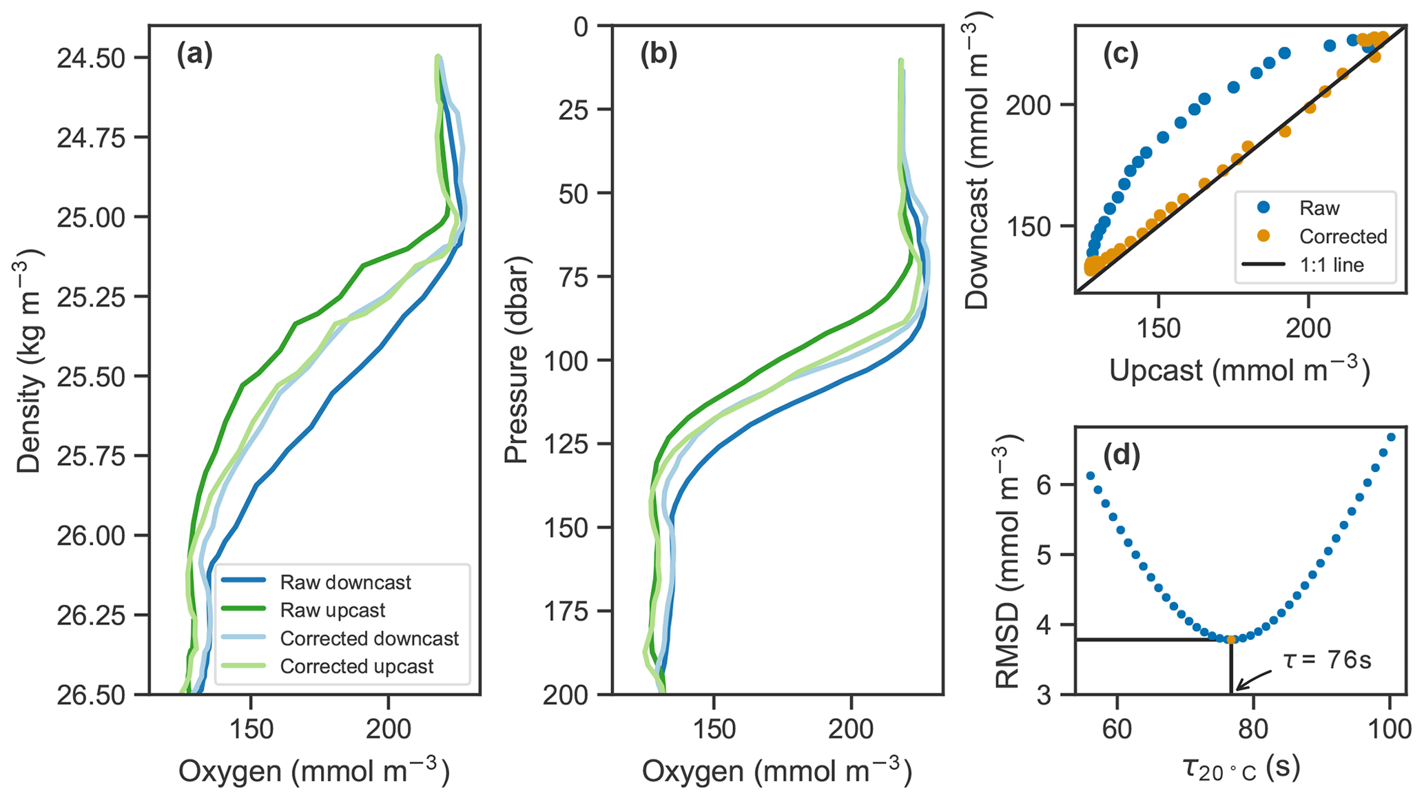
https://bg.copernicus.org/articles/17/4119/2020/bg-17-4119-2020-f02

Figure 2Example of raw oxygen measurements from a downcast and an upcast (darker blue and green lines, respectively) and corrected profiles (lighter lines) in (a) density and (b) pressure coordinates. (c) Upcast and downcast (top 150 m) plotted against each other with raw data in blue and corrected data in orange. (d) The root-mean-square difference (RMSD) between the upcast and downcast after correcting casts for a range of time constants, τ, showing the optimal τ value at 20 ^∘C in this case of 76 s in orange.

Download

Observation of an oxygen profile by the optode can be described as a low-pass filter of the true oxygen profile (Bittig et al., 2014), given by the following differential equation:

\begin{matrix} (1) & h (t) = f (t) - τ \frac{\partial h}{\partial t}, \end{matrix}

where h(t) is the oxygen measured by the optode at time t, f(t) is the true oxygen concentration (both in mmol O₂ m⁻³), and τ is the effective response time (s) which depends on the sensor and its environment. This differential equation can be solved using a Laplace transform as follows (see Appendix A1 for the full derivation):

\begin{matrix} (2) & h (t) = f (0) e^{- t / τ} + \frac{1}{τ} \int_{0}^{t} f (t - u) e^{- u / τ} d u . \end{matrix}

The first term represents the decaying initial measurement by the sensor, where we have assumed that at time t=0 the sensor reads the true oxygen concentration correctly (i.e., h(0)=f(0)). The second term is the convolution of the true oxygen concentration and a decaying exponential which represents the transfer function of the sensor (i.e., the delay in measuring the true concentration). Therefore, the observation h can be expressed more generally as a convolution $h = f * g$ , where h represents the measurement, f is the true concentration, and g is a function representing the response of the sensor (unitless). To recover the correct oxygen profile, the deconvolution of the profile and the sensor must be performed. This is possible if the observation h (with time stamps for each data point) and the equation describing the sensor transfer function g are known. From Eq. (2), the sensor's transfer function can be defined as

\begin{matrix} (3) & g (t) = \frac{1}{τ} e^{- t / τ} . \end{matrix}

This provides the mathematical basis for correcting the sensor hysteresis.

Up to now, the sensor theory has been discussed in continuous time. In order to apply a correction to the data, the formalism must be discretized. We are discretizing the equation in Laplace space and then transforming it into the more familiar time domain. By taking the Laplace transform of the transfer function (Eq. 3) and assigning the proper Laplace variable and then discretizing the Laplace transform using a bilinear transformation and performing the inverse discrete Laplace transform (or Z transform; see Proakis and Manolakis, 1996; Antoniou, 2018), the following relationship can be derived:

\begin{matrix} (4) & h_{n} = a h_{n - 1} + b (f_{n} + f_{n - 1}), n = 1, \dots, N, \end{matrix}

with the unitless coefficients

b = {(1 + 2 \frac{τ}{t_{n} - t_{n - 1}})}^{- 1}, a = 1 - 2 b .

See Appendix A2 for the detailed derivation. Equation (4) can be rewritten in the same form as provided by Bittig and Körtzinger (2017), their Eq. (A3),

\begin{matrix} (5) & \frac{f_{n} + f_{n - 1}}{2} = \frac{1}{2 b} (h_{n} - a h_{n - 1}), \end{matrix}

and is a recursive formulation similar to the one used for correction of thermal mass in conductivity cells (Lueck, 1990; Lueck and Picklo, 1990). Since deconvolution is known to amplify random errors, which is especially relevant where the truth f(t) is convolved with the transfer function of an instrument g(t), smoothing of the raw signal may improve the final estimate (Wiener, 1964).

Equation 4 provides the recipe for correcting for the slow sensor response. Two essential ingredients for applying this correction, in addition to the raw measurements themselves, are knowledge of their time stamps and of the effective response time, τ. In reality, the response time also depends on ambient temperature, as described by Bittig et al. (2018). The above formalism can be applied for the response time at a reference temperature to accommodate the temperature dependence. Next, an in situ method for determining the measurement's effective response time is described.

3.2 In situ determination of measurement response time

In situ determination of the measurement's effective time constant is possible if consecutive upcasts and downcasts are recorded, assuming the oxygen profile does not significantly change between consecutive casts. In our case, the top 200 m was sampled on average within 70 min during continuous sampling, and time stamps were transmitted. Determination of the time constant can be thought of as an inverse problem where the correction method derived in Sect. 3.1 is applied to a range of plausible time constants. The one that minimizes the discrepancy between consecutive upcasts and downcasts is the optimal value and taken as the effective response time. Here, the temperature dependence of the response time is taken into account by optimizing for the effective boundary layer thickness. More specifically, we applied the correction method from Eq. (5) while systematically sweeping over a range of boundary layer thickness values. Using the lookup table provided by Bittig and Körtzinger (2017) and the temperature profile measured by the float, these can be related to the effective response time which is then used to correct the oxygen profiles. The root-mean-square difference (RMSD) between upcasts and downcasts was calculated by matching consecutive profiles at each density level from the surface to 1027 kg m⁻³, and the one with the minimum RMSD was taken as the effective boundary layer thickness. An illustration of the process is shown in Fig. 2d. The effect of the correction is visible in Fig. 2a–c.

Since the deconvolution is known to amplify high-frequency noise, the profiles were smoothed using a first-order low-pass Butterworth filter (butter(1, 0.7) in MATLAB) prior to performing the correction. This was particularly important for the downcasts. Profiling floats typically only measure on the upcast because most of the sensors are located near or at the top of the float, allowing the sensors to measure undisturbed water on the upcasts. On the downcasts, water is thought to have been churned up by the body of the float increasing random errors. In our case, smoothed profiles agreed more closely in the oxygen gradient, and their RMSD after correction was slightly reduced.

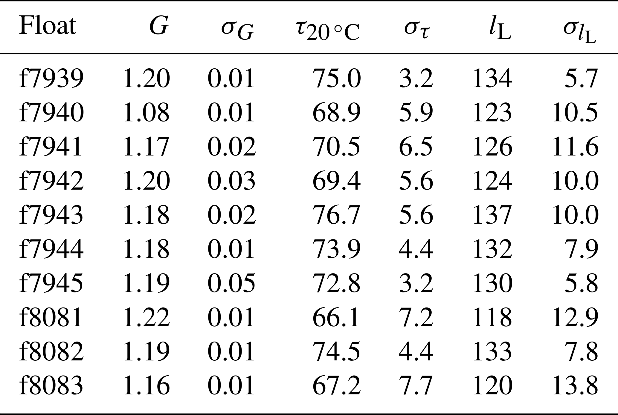
For clarity, we provide the response time values at a reference temperature (T=20 ^∘C) rather than the boundary layer thickness. The calculations were done for each pair of consecutive upcasts and downcasts and down- and upcasts, resulting in a population of N−1 time constants for each set of N float profiles. The median time constants for each float are listed in Table 2. Median optimal time constants ranged from 67.2 to 76.7 s across the 10 floats, and the standard deviation of those values was as low as 3.2 s and as high as 7.7 s. Similar to the gain correction (see Sect. 2.2), the median optimal response time of each float was applied to all profiles from that float.

Table 2Mean gain values derived from in-air measurements (G, unitless), median time constants ( $τ_{20^{\circ} C}$ , s), and median boundary layer thickness values (l_L, µm) for each float with standard deviations (σ, appropriate units).

Download Print Version | Download XLSX

The variation of effective response time from profile to profile for one float is due to its dependence on various factors, chiefly among them is the flow speed of ambient water over the sensor. Next, we analyze how deviations from the average profiling speed and random errors manifest themselves in the final corrected oxygen product.

3.3 Propagation of response time error and sensor noise

The optode measurements are subject to systematic and random errors. The response time may change with variations in temperature, salinity, pressure, and most importantly flow speed of ambient water at the sensing interface. The latter is highly dependent on profiling velocity which varied from 1.4 to 26.5 cm s⁻¹ with a mean of 12.2 cm s⁻¹ for our floats. As we account for variations in temperature already, we analyze how variations in response time due to changes in boundary layer, as well as random measurement errors, propagate through the correction process. This is done using an idealized oxygen profile sampled as it would be by a float but with different known errors applied.

The response time effect is simulated by applying a discretized version of equation (Eq. 1):

\begin{matrix} (6) & h_{n} = α f_{n} + (1 - α) h_{n - 1} where α = \frac{Δ t}{τ + Δ t}, \end{matrix}

where h_n and f_n are the measurement and true oxygen concentration at time step n, respectively. At t=0 we assumed oxygen is correctly measured; i.e., h(0)=f(0). The right-hand-side term with f_n represents the real-time contribution to the measurement, and the term with h_n−1 represents the sensor's memory of previous measurements. The recursive structure of the measurement filter results in an exponentially weighted moving average with an infinite averaging window in time. A full derivation is given in Appendix B.

We simulated the generation of optode measurements by prescribing a profiling velocity of 15 cm s⁻¹, taking a measurement every 5 m (roughly the vertical resolution of the floats), assigning a time stamp to each oxygen datum, and then running the model output through the measurement filter using a prescribed response time (temperature is assumed to be constant here). Known errors were added to this measurement process as random perturbations of the response time and as random noise added to the measured oxygen values. The two error sources were examined individually for a range of standard deviations to systematically analyze the effect of each error type. Response times τ (s) were chosen from a normal distribution with a mean of 75 s and standard deviations ranging from 0 to 15 s. Sensor noise errors ϵ (mmol m⁻³) were chosen from a normal distribution with mean zero and standard deviations ranging from 0 to 1.5 (mmol m⁻³). Following the simulated measurement, the measured profiles underwent the same correction process as the float data: first a 7 pt smoothing and then the response time correction using the expected value of 75 s. Different magnitudes of errors were tested, and for each trial the measurement and correction process was repeated 50 times.

https://bg.copernicus.org/articles/17/4119/2020/bg-17-4119-2020-f03

Figure 3(a) Simulated profile measurements (blue) of the true oxygen profile (black) for 50 different response times drawn randomly from a normal distribution with a standard deviation of 15 s and mean of 75 s, and corrected measurements using a response time of 75 s (orange). (b) Deviations of corrected profiles from the true profile, with line color representing the randomly drawn response time. (c) Simulated measurement and correction of profiles using a response time of 75 s, with random noise added from a normal distribution with a standard deviation of 1 mmol m⁻³ and mean of 0 mmol m⁻³. (d) Deviations of corrected profiles in (c) from the true profile.

Download

Panels (a) and (b) in Fig. 3 show the measured and corrected profiles for the widest distribution of response time errors tested (σ_τ=15 s), in the absence of random sensor error. In gradient-free segments of the oxygen profile, the error has little to no effect, while larger deviations from the true profile occur in the high-gradient segments of the profile, with a maximum deviation of almost 10 mmol m⁻³. In contrast to the response time error, random sensor error (Fig. 3c and d) does not have a localized effect on the profile, but the errors appear to be amplified by the correction process. Figure 4 summarizes the two error analyses by showing the standard deviation of the deviation profiles, σ_dev, for increasingly wide distributions of response time and random errors. For response time errors, the distribution of deviations has a maximum value exceeding 1.0 mmol m⁻³. This demonstrates that, despite a range of response times estimated for the floats, the corrected profiles are close to the true oxygen profile. For random noise, an amplification of the errors by a factor of 3 occurs through the correction process. This amplification is consistent with theoretical consideration (see Appendix C).

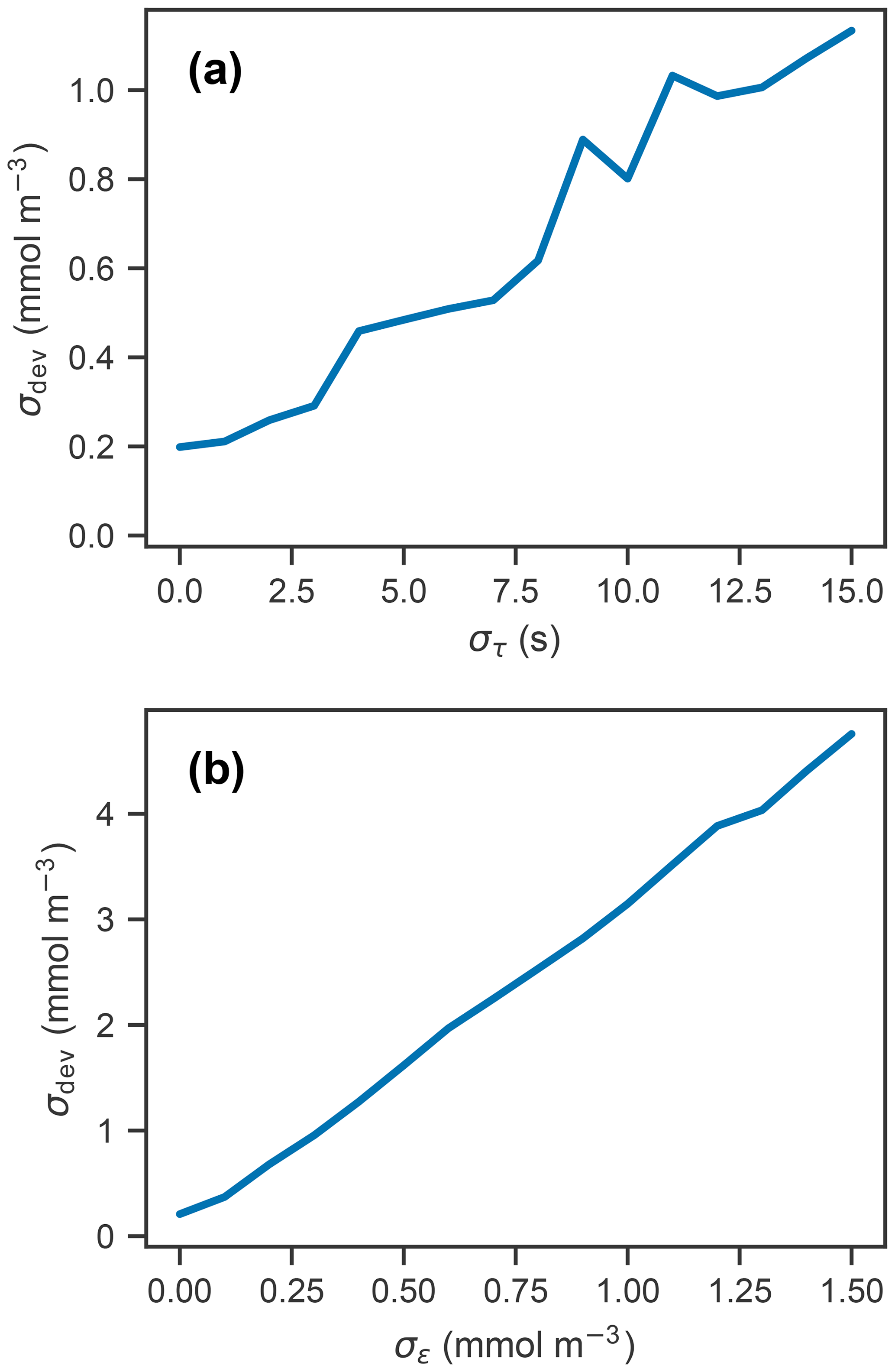
https://bg.copernicus.org/articles/17/4119/2020/bg-17-4119-2020-f04

Figure 4Standard deviation of the error profiles for increasingly wide distributions of (a) response time and (b) random error. For random errors, σ_dev increases linearly with σ_ϵ, with a slope of 3.09 (unitless).

Download

3.4 Discussion

The slow response time of the optode is considered a prominent source of error when measuring oxygen on floats (see Plant et al., 2016; Johnson et al., 2017) but is often not rigorously corrected for. One reason is that the time stamps of the oxygen measurements are not typically transmitted (Johnson et al., 2017). Another reason is that the sensor response time is difficult to characterize without knowledge of the true profile. To minimize response time errors, some optodes are pumped to significantly increase the flow speed at the interface between sensing foil and ambient seawater and thus decrease boundary layer thickness and the effective response time. However, even pumped optodes have a characteristic response time, albeit reduced. In addition, pumped optodes have the disadvantages of consuming more energy and being unable to record in-air measurements for calibration.

Plant et al. (2016) cited response time errors as the cause of unrealistically large values of positive NCP just above the mixed layer and negative NCP below. They chose to correct mixed-layer oxygen by extending surface oxygen values on the assumption that oxygen is completely uniform in the mixed layer. However, a full correction using the filtering solution provided by Bittig et al. (2014) could have improved the estimates not only at the mixed-layer interface but also for the entire profile. While oxygen values near the base of the mixed layer were the most obvious evidence of errors induced by the response time, any oxygen gradient would have been subject to the effects of sensor response time as well and thus would have been improved by the inverse filtering correction.

Johnson et al. (2017) compared oxygen measurements made by floats in the Southern Ocean and Winkler titrations (Winkler, 1888; Carpenter, 1965) from bottle samples at deployment stations. While optode-measured oxygen generally agreed very well with the Winkler measurements, the majority of error was concentrated around high-gradient areas. Response time corrections could not be performed in this case because the floats did not transmit time stamps for each oxygen measurements and only the upcasts were transmitted. As previously stated, time stamps and knowledge of the measurement's time constant are the two key pieces of information required to make the correction. Measurement of consecutive upcasts and downcasts allows for an in situ determination of the effective response time as shown here.

The effective response times derived here are much longer than the sensor-inherent response times reported on the Aanderaa data sheet, but this discrepancy is not surprising. The data sheet provides an estimate of the inherent sensor response time (25 s for 63 % of the signal), which is calculated by subjecting the sensor to a sudden step change in oxygen (by plunging from air into water). Here we have determined the effective response time of the measurement in situ, which also accounts for diffusion through the boundary layer at the sensing interface. This boundary-layer effect is significant for typical float velocities. The 70 s response times found here are fully consistent with previously reported response times of 15–45 s for CTD measurements (Bittig et al., 2014) and 60–95 s for profiling floats in the subtropical ocean (Bittig and Körtzinger, 2017).

Subjecting simulated measurements to varying effective response times and random sensor errors showed that the combined effects of these two sources of error can cause significant deviations between the corrected and true profiles (Fig. 3). The 50 repeated measurements of the oxygen profile with a response time error (standard deviation) of 10 s and random errors on the order of 1.0 mmol m⁻³ resulted in deviations of approximately 1.0 and 3.0 mmol m⁻³, respectively (Fig. 4). Taking these two sources of error and considering them independent from one another, the combined error estimate is between 3 and 4 mmol m⁻³, which is significant considering the precision needed to detect diurnal cycles in oxygen.

Bittig et al. (2018) stated that the relation between the boundary layer thickness and float profiling velocity must be established on a case-by-case basis depending on the platform characteristics and optode attachment with respect to flow direction. For this analysis, effective time responses of the optode on the upcasts and downcasts are treated to be equal. In reality, flow around the optode may not be identical for the two cast directions; however, the impact of this difference on the corrections is unknown.

The technique we propose for determining the effective time constant is a simple and practical method for in situ application and more straightforward than characterizing flow surrounding the optode. It can easily be performed by any end user of optode data from floats, as long as time stamps and occasional upcasts and downcasts are transmitted. In our case, the difference between the measured and corrected profiles is substantial. In the study region, where the maximum oxygen gradient of each profile averaged 3.8 mmol m⁻³ dbar⁻¹, median differences between observed and corrected profiles ranged from 31 to 43 mmol m⁻³ at the maximum gradient. For a given time constant, the magnitude of the difference between corrected and uncorrected profiles varies linearly with gradient strength.

The key assumption made in our method for in situ response time determination is that the upcasts and downcasts should match. We performed this comparison in pressure space. Conducting the analysis in density space instead would be a natural extension and may avoid potential errors resulting from isopycnal movements. A potential limitation of the method is that the float measures disturbed water during the downcast, as the optode sits at the top of the float. Such a change in the flow field at the sensor interface may affect the response time during downcasts. It seems unlikely that this has a large effect on our results, but the response times for upcasts and downcasts are probably not exactly the same.

4 Biological and physical drivers of dissolved oxygen variations

4.1 Measurement of diurnal oxygen cycles

Next, we attempt to estimate GPP, R, and NCP from hysteresis-corrected oxygen measurements collected during continuous-mode profiling. The approach relies on an ability to determine diurnal variations in oxygen in the euphotic zone and the following assumptions. During daylight hours, oxygen increases at a rate proportional to the difference between GPP and R, while during the night oxygen decreases at the rate R. Then, GPP can be estimated from diurnal oxygen cycles of this idealized structure. This is essentially what Briggs et al. (2018) assumed when they applied a linear fit to their nighttime data, where the slope represents the respiration rate, and extrapolated forward to noon the next day to project the dissolved oxygen concentration in the absence of any production (Fig. 5, dashed lines). An estimate for morning GPP was then obtained with the help of a second linear fit applied to the daytime data where the difference between the extrapolated nighttime fit and the value of the daytime fit at noon represents oxygen production in the morning (Fig. 5, light green bars). The oxygen produced in the second half of the day can be calculated in a similar manner (Fig. 5, dark green bars). No correction for air–sea flux was performed on the data as the expected change was comparatively small (Gordon, 2019).

https://bg.copernicus.org/articles/17/4119/2020/bg-17-4119-2020-f05

Figure 5Schematic showing method for calculating GPP and R using oxygen data (points) after Briggs et al. (2018). Respiration rates are determined as nighttime slopes (solid black lines), which are then projected forward and backward in time (dashed black lines). The differences between these projections and oxygen at noon observed yields the morning and afternoon GPP (light and dark green bars respectively).

Download

An observed time series of mean oxygen over the upper 150 m of the water column (but excluding measurements within the uppermost 5 m where the pumped CTD automatically turns off as it approaches the sea surface) from one of the continuous-mode sampling periods is shown as example in Fig. 6. In the time series, the upcasts and downcasts are brought into agreement by removing the constant bias between them, which exists despite the response time correction. While oxygen is often changing periodically with increases during the day and decreases during the night, there also are several instances when oxygen changes cannot be reconciled with the expected day–night pattern of a biologically driven cycle. Light and dark red bars represent unrealistic negative gross production values (GPP, by definition, must be positive). This time series illustrates that, in the study region, estimating production from diurnal oxygen changes is not straightforward. It appears that processes other than biological production and consumption are affecting oxygen, complicating the expected signal. We obtained similar results during other periods and for other floats. A confounding physical driver of short-term oxygen variations is explored in Sect. 4.2.

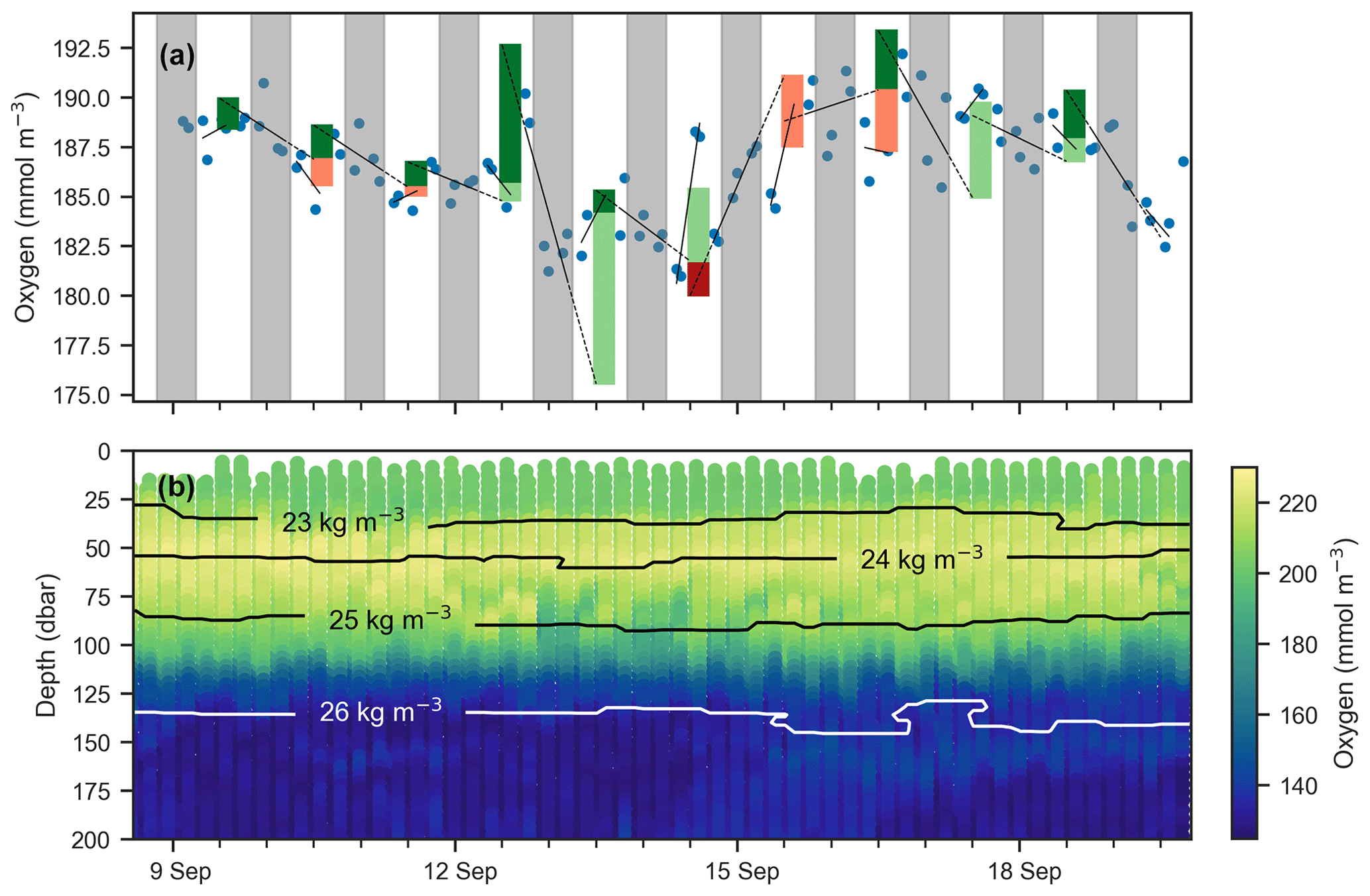
https://bg.copernicus.org/articles/17/4119/2020/bg-17-4119-2020-f06

Figure 6(a) Mean oxygen in the euphotic zone for continuous-mode measurements in September from float f8081, with attempts to estimate GPP. The legend is the same as Fig. 5, but orange and red bars indicate when the method obviously fails because other processes than production and respiration are driving changes in oxygen. Gray shaded sections show local nighttime. (b) Oxygen data over the same period with overlaid isopycnal contours.

Download

4.2 Physically induced variations in dissolved oxygen

Vertical oscillations of isopycnals may occur in ocean environments due to several processes including internal or near-inertial waves, barotropic or baroclinic tides, and mesoscale eddies and may influence dissolved oxygen dynamics in the euphotic zone. Such isopycnal displacements will push the oxygen gradient up and down, creating a periodic signal in vertically integrated oxygen. Although a spectrum of internal motions are present (Garrett and Munk, 1972, 1979), in this section we examine an example that likely represents a near-inertial wave as the observed oscillations have a period of 24 h, corresponding to the Coriolis frequency at 30^∘ N (Alford et al., 2016). Caution must be exercised as to not misconstrue the physical oscillatory signal with a biological one.

Vertical oscillations were visible in our float data in many instances. As an example, a 3 d period immediately following the deployment of float f7940 on 2 May 2017 is examined here. This float was deployed shortly before passage of an atmospheric front with elevated wind speeds up to about 35 km h⁻¹. Vertical oscillations are apparent by coincident up and down movements of the oxygen gradient moving in concert with isopycnals (Fig. 7). A tight correlation of oxygen isolines and isopycnal (or isotherm) depths identifies when physical oscillations are driving changes in oxygen.

The depths of the 20.6 ^∘C isotherm and 142.6 mmol O₂ m⁻³ iso-concentration are highly correlated over this time period (Fig. 7c, r=0.97, p<0.01). The time series of these depths are also highly correlated with the time series of integrated oxygen (Fig. 8, r=0.74, p<0.01). The extrema are aligned as well, as the maximum depths of the isotherm correspond with the maximum values of integrated oxygen, and similarly minimal depths correspond to integrated oxygen minima, occurring near noon and at midnight, respectively.

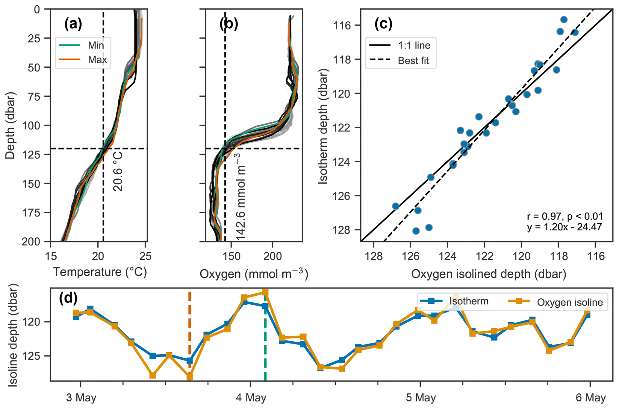
https://bg.copernicus.org/articles/17/4119/2020/bg-17-4119-2020-f07

Figure 7Covariation of isotherm and iso-concentration depths. (a–b) Profiles of temperature and dissolved oxygen, where the profiles with the minimum and maximum depths of the 20.6 ^∘C isotherm and 142.6 mmol O₂ m⁻³ iso-concentration are shown in green and orange respectively, and all other profiles are shown on a gray color scale indicative of time, with lighter shades indicating older and darker shades more recent measurements. (c–d) Depths of the isotherm and iso-concentration plotted against each other in (c) and as a time series in (d), showing their covariation.

Download

https://bg.copernicus.org/articles/17/4119/2020/bg-17-4119-2020-f08

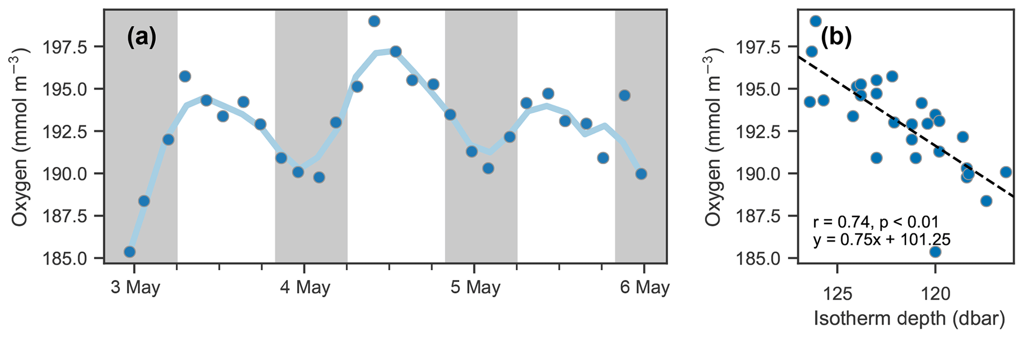
Figure 8Isotherm depth and mean oxygen comparison. (a) Time series of mean oxygen between 25 and 150 dbar. A period of about 24 h is observed; however, it is not in phase with the day–night cycle (nighttime indicated by shaded areas) as would be expected for a biological signal. (b) Scatter of mean oxygen concentration against isotherm depth (see Fig. 7d).

Download

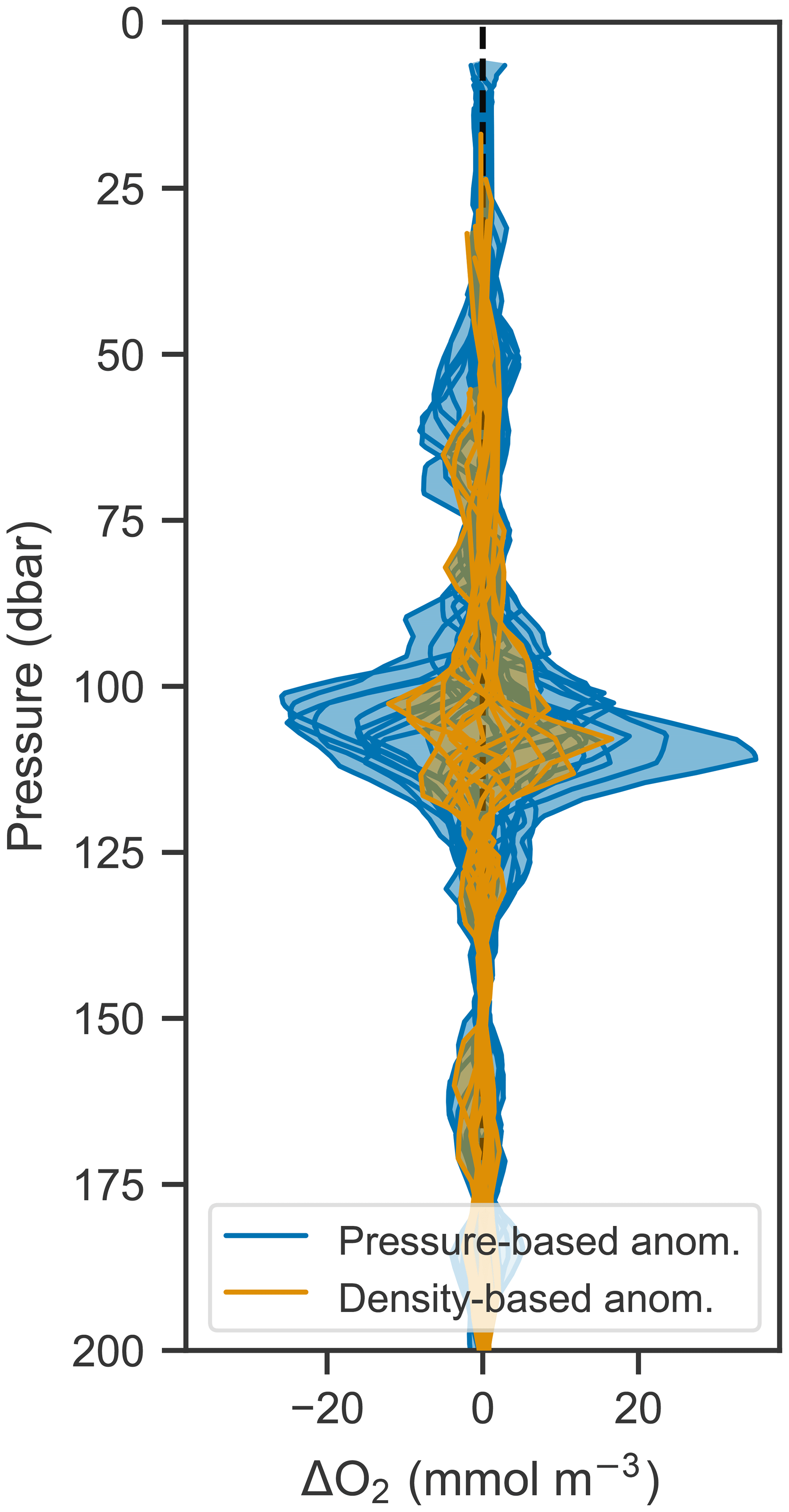
Since the vertical movement of isopycnals and oxygen isolines creates a tight correlation between the two, it should be possible to remove the variability due to vertical motions by analyzing changes in oxygen in density space rather than pressure space. This is done by calculating the anomaly (by subtracting an average profile over a time period from each constituent profile) at each density level and then mapping that anomaly back to pressure space. Figure 9 shows the anomalies calculated in pressure and density space compared to each other. Anomalies calculated in density space are significantly smaller, indicating that most of the variability in oxygen can be accounted for by corresponding changes in density. This technique offers a path to removing the oscillatory signal and therefore isolating underlying signals such as biological production. In this case, however, the remaining anomaly is on the order of expected errors based on the analysis performed in Sect. 3.3, and so a biological signal cannot be discerned in light of the accumulated error.

https://bg.copernicus.org/articles/17/4119/2020/bg-17-4119-2020-f09

Figure 9Anomalies of oxygen profiles from Fig. 7b shown in pressure (blue) and density (orange) space.

Download

4.3 Discussion

The data and analysis presented in this section show that diurnal changes in oxygen can be measured with a profiling float; however, the changes observed here could not unequivocally be linked to biological production and respiration. This made estimates of daily GPP, R, and NCP based on these observations unreliable or impossible. Compared to previous work by Briggs et al. (2018), which focused on diurnal oxygen cycles in the North Atlantic spring bloom, the Gulf of Mexico has relatively low production. Nicholson et al. (2015) studied diurnal oxygen cycles in a similarly low productivity region in the subtropical North Pacific but accumulated and averaged many days in order to derive an estimate of production. In a more recent study, Barone et al. (2019) were able to resolve variability in production on the timescale of 1 week in the same region.

The location of the floats and the timing of the continuous-mode observations also contributed to the difficulty in estimating production. Continuous mode was turned on when strong storms were passing through the Gulf of Mexico, likely causing physical drivers to dominate variations in oxygen. Additionally, the floats were deployed near the shelf break, and topography is a known factor contributing to the formation of internal motions (Alford et al., 2016) under external physical forcings. Furthermore, the temporal resolution was on the low end for making diurnal measurements. In continuous mode, the floats still recorded full profiles to at least 1000 m because of other research objectives. In a study more directly focused on diurnal oxygen cycles, profiling to only 200 to 300 m would significantly increase the temporal resolution of the oxygen time series, while still capturing the entire euphotic zone.

Vertical oscillations, and other physical drivers, can influence euphotic-zone oxygen with implications for the measurement of biologically driven changes. In attempting to measure biological productivity using oxygen, it is important to understand such effects and take them into consideration. Vertical oscillations can be identified in float data by observing the synchronous movement of physical and biochemical variables in the water column. When identified, the characteristically tight correlation of density and oxygen may still allow for the isolation of the underlying biological signal. In our case, although the vertical oscillation signal can mostly be captured by variations in density (Fig. 9), the remaining signal cannot always be attributed to biological changes in the water column. For our data, this analysis showed anomalies on the same scale as the expected error from the oxygen optode. In Plant et al. (2016), evidence of internal waves was also present in the data, and a similar method was used to remove this signal. In their case, using density to map the observations to a physical model that did not include vertical oscillations, it was possible to isolate the biological signal.

Elevated winds acting on this region with variable topography can generate internal oscillations with a period of about 24 h (determined by the Coriolis frequency at 30^∘ N, where the autonomous floats in this study were deployed). Without consideration of the physical data, if this oscillation was aligned with the expected day–night cycle, it could falsely appear to be driven by biological productivity. The diurnal-scale period of the internal oscillations could also be problematic if production is estimated by accumulating and averaging data as in Nicholson et al. (2015). That study quantified average NCP over 110 d by accumulating multiple glider measurements of oxygen into one 24 h cycle. Only oxygen data that fit the theoretical biological curve defined a priori to a satisfactory degree (p<0.05) were accumulated (73 of 110 d satisfied this condition). This approach could allow physically driven oscillations that are aligned with the day–night cycle to be attributed to biology.

5 Conclusions and recommendations

In the Introduction, we posed two sets of questions relevant for the estimating of NCP and R from the diurnal oxygen cycle measured by continuously profiling autonomous floats. The first set addressed the technical question of whether the sensor and platform can take sufficiently frequent and accurate measurements. The second set contained oceanographic questions about what primary physical or biological processes drive changes in dissolved oxygen and how they manifest themselves in the data. Addressing the first led to the development of a novel method for determining the effective in situ time constant of an oxygen optode deployed on a profiling float, without needing to characterize the physical flow around that sensor. The second was addressed by analyzing physical and oxygen measurements from our study in the Gulf of Mexico and provides context and techniques to future studies seeking to quantify production using profiling floats.

Oxygen optodes are challenged to make accurate measurements in gradients because of their slow response time. However, the resulting errors can be corrected if time stamps of the measurements and the effective response time are known. We developed an optimization procedure to determine the effective time constant in situ by using both the upcasts and downcasts measured by the floats. The effective time constant determined in the field represents the combination of the inherent sensor response time and the response time that results from boundary layer effects. The time constants derived by this method are similar to estimates provided in the previous literature. While the oxygen measurements were improved significantly by the correction procedure, remaining errors, especially near gradients, may prohibit reliable production estimates in low-productivity environments or where physical processes have large effects on the oxygen signal.

Given the small productivity of the Gulf of Mexico, oxygen optodes on autonomous floats were not able to provide sufficient precision to estimate production on a diurnal scale, likely because of a combination of sensor error and nonbiological changes in oxygen. For processes like the vertical oscillation of isopycnals, analysis in density space can reveal underlying signals, and inspection of anomalies may be useful in calculating diurnal-scale biological changes in oxygen.

The need for highly accurate oxygen measurements when estimating production from autonomous platforms leads to the following recommendations for future deployments of autonomous floats with oxygen optodes:

Include time stamps for every oxygen measurement on float data transmission. The corrections discussed and applied here must be performed on oxygen as a time series. Correction for sensor response time is impossible without this information.
Program the float mission to include a calibration period upon float deployment where both upcasts and downcasts are recorded. This will provide a very practical and robust method to calculate the effective in situ response times.

This work contributes to improved quality control of oxygen measurements by optodes, may stimulate further use of profiling floats for observing diurnal cycles of dissolved oxygen for calculation of GPP and R, and enhances our understanding of processes driving changes in oxygen in the shelf break region in the northern Gulf of Mexico. Our methods and findings are applicable to other regions.

Appendix A: Optode mathematical formalism

A1 Laplace solution

Recall filter differential equation

\begin{matrix} (A1) & h (t) = f (t) - τ \frac{\partial h}{\partial t} . \end{matrix}

This can be rewritten as an initial value problem assuming that the first measurement has the correct value (h(0)=f(0)):

\begin{matrix} (A2) & h^{'} + \frac{1}{τ} h = \frac{1}{τ} f . \end{matrix}

Taking the Laplace transform of the above equation, we obtain

\begin{array}{l} (A3) & L {h^{'} + \frac{1}{τ} h} = L {\frac{1}{τ} f}, \\ (A4) & s H (s) - h (0) + \frac{1}{τ} H (s) = \frac{1}{τ} F (s) . \end{array}

Rearranging to solve for H(s) and substituting h(0)=f(0) yields

\begin{matrix} (A5) & H (s) = (\frac{1}{s + \frac{1}{τ}}) f (0) + \frac{1}{τ} (\frac{1}{s + \frac{1}{τ}}) F (s) . \end{matrix}

For the first term, we can take the inverse Laplace transform directly, as we recognize the following form:

\begin{matrix} (A6) & L {e^{α t}} = \frac{1}{s - α} . \end{matrix}

For the second term, because f(t) is unknown, the solution is written as a convolution. The final solution is

\begin{matrix} (A7) & h (t) = f (0) e^{- t / τ} + \frac{1}{τ} \int_{0}^{t} f (t - u) e^{- u / τ} d u . \end{matrix}

A2 Discretized solution

The transfer function of the oxygen optode is expressed as

\begin{matrix} (A8) & g (t) = \frac{1}{τ} e^{- t / τ}, \end{matrix}

and the Laplace transform of this expression is

\begin{matrix} (A9) & G (s) = L {g (t)} = (1 + s τ)^{- 1} . \end{matrix}

In order to convert this continuous-time domain (analog) filter to a discrete-time domain (digital) filter, we apply a bilinear transform. The bilinear transform is a first-order approximation of making the change of variables z=e^sΔt (or $s = \frac{1}{Δ t} \ln (z)$ ), where Δt is the time between measurements. This approximation is made by taking the first term in the Taylor series of the change of variables:

\begin{matrix} (A10) & s = \frac{2}{Δ t} \frac{1 - z^{- 1}}{1 + z^{- 1}} . \end{matrix}

Substituting the above into Eq. (A9) yields

\begin{array}{l} (A11) & G (z) & = G (s) |_{s = \frac{2}{Δ t} \frac{1 - z^{- 1}}{1 + z^{- 1}}} \\ (A12) & = {(1 + \frac{2 τ}{Δ t} \frac{1 - z^{- 1}}{1 + z^{- 1}})}^{- 1}, \end{array}

which can be rearranged to

\begin{matrix} (A13) & G (z) = \frac{{(1 + 2 τ / Δ t)}^{- 1} (1 + z^{- 1})}{1 + \frac{1 - 2 τ / Δ t}{1 + 2 τ / Δ t} z^{- 1}} . \end{matrix}

Finally, substituting in $b = (1 + 2 τ / Δ t)$ and $a = 1 - 2 b$ yields

\begin{matrix} (A14) & G (z) = \frac{b (1 + z^{- 1})}{1 - a z^{- 1}} . \end{matrix}

The inverse Z transform (i.e., discrete inverse Laplace transform) of Eq. (A14) yields Eq. (4).

Appendix B: Discretized optode filter

Recall filter differential equation

\begin{matrix} (B1) & h (t) = f (t) - τ \frac{\partial h}{\partial t} . \end{matrix}

Discretizing the above equation using finite difference

\begin{matrix} (B2) & h_{n} = f_{n} - τ \frac{h_{n} - h_{n - 1}}{Δ t}, \end{matrix}

then rearranging and factoring out h_n, yields

\begin{matrix} (B3) & h_{n} (1 + τ Δ τ) = f_{n} + \frac{τ}{Δ t} h_{n - 1} . \end{matrix}

The solution

\begin{matrix} (B4) & h_{n} = (\frac{Δ t}{τ + Δ t}) f_{n} + (\frac{τ}{τ + Δ t}) h_{n - 1} \end{matrix}

can be derived with some simple algebra. Defining $α = \frac{Δ t}{τ + Δ t}$ yields

\begin{array}{l} (B5) & h_{n} & = (\frac{Δ t}{τ + Δ t}) f_{n} + (\frac{τ + Δ t}{τ + Δ t} - \frac{Δ t}{τ + Δ t}) h_{n - 1}, \\ (B6) & h_{n} & = α f_{n} + (1 - α) h_{n - 1} . \end{array}

Appendix C: Error propagation

Adding error into the inverse filtering solution (Eq. 5) as an addition to the observations yields

\begin{matrix} (C1) & \frac{f_{n} + f_{n - 1}}{2} = \frac{1}{2 b} (h_{n} - a h_{n - 1}) + \frac{1}{2 b} (ϵ_{n} - a ϵ_{n - 1}), \end{matrix}

where ϵ_n is the error at time step n. Our goals is to obtain the coefficient in front of the error term. Assuming that the error ϵ is independent and identically distributed, the variance of this additional term is as follows:

\begin{matrix} (C2) & σ_{f}^{2} = \frac{1 + a^{2}}{4 b^{2}} σ_{ϵ}^{2} . \end{matrix}

Replacing $a = 1 - 2 b$ and rearranging yields

\begin{matrix} (C3) & \frac{1 + a^{2}}{4 b^{2}} = \frac{1}{2} b^{- 2} - b^{- 1} + 1 . \end{matrix}

Replacing $b^{- 1} = 1 + 2 \frac{τ}{Δ t}$ and simplifying we obtain

\begin{matrix} (C4) & \frac{1}{2} b^{- 2} - b^{- 1} + 1 = \frac{1}{2} (1 + 4 \frac{τ^{2}}{Δ t^{2}}) . \end{matrix}

The variance of the error will by multiplied by the above factor. The standard deviation therefore is amplified by its square root:

\begin{matrix} (C5) & \frac{σ_{f}}{σ_{ϵ}} = \sqrt{\frac{1}{2} (1 + 4 \frac{τ^{2}}{Δ t^{2}})} . \end{matrix}

The above gives the general result. For our error analysis, τ=75 s and Δt=33 s, we obtain an amplification of

\begin{matrix} (C6) & \begin{aligned} \sqrt{\frac{1}{2} (1 + 4 \frac{τ^{2}}{Δ t^{2}})} & = \sqrt{\frac{1}{2} (1 + 4 \frac{(75)^{2}}{(33)^{2}})} \\ \approx 3.3 . \end{aligned} \end{matrix}

The above derivation does not account for any smoothing, and the result in Eq. (C6) is consistent with our numerical results

Code availability

MATLAB code for determining sensor response time is available at https://doi.org/10.5281/zenodo.3975671 (Gordon et al., 2020 b).

Data availability

Float data are available at https://doi.org/10.5281/zenodo.3890239 (Gordon et al., 2020 a).

Author contributions

CG and KF formulated the idea and research questions underlying this study and cowrote the manuscript. CG carried out processing and quality control of the oxygen data, developed the correction method, and carried out all analyses. LKS and JB prepared the cruise, deployed the float with assistance by CG and KF, and oversaw data transmission. CR made essential contributions to the error analysis in Sect. 3.3.

Competing interests

The authors declare that they have no conflict of interest.

Special issue statement

This article is part of the special issue “Biogeochemistry in the BGC-Argo era: from process studies to ecosystem forecasts (BG/OS inter-journal SI)”. It is not associated with a conference.

Acknowledgements

The authors wish to thank Giorgie Dall'Olmo, Henry Bittig, and David Nicholson for their insightful comments which helped improve this paper. Henry Bittig contributed to incorporating the temperature dependence in the analysis during revision, which is gratefully acknowledged.

Financial support

This research has been supported by the Gulf of Mexico Research Initiative (grant no. GoMRI-V-487).

Review statement

This paper was edited by Carol Robinson and reviewed by Henry Bittig and Giorgio Dall'Olmo.

References

Alford, M. H., MacKinnon, J. A., Simmons, H. L., and Nash, J. D.: Near-Inertial Internal Gravity Waves in the Ocean, Annu. Rev. Mar. Sci., 8, 95–123, 2016. a, b

Antoniou, A.: Digital filters: Analysis, Design, and Signal Processing Applications, 2nd Edn., McGraw-Hill, 2018. a

Barone, B., Nicholson, D., Ferrón, S., Firing, E., and Karl, D.: The estimation of gross oxygen production and community respiration from autonomous time-series measurements in the oligotrophic ocean, Limnol. Oceanogr.-Meth., 17, 650–664, 2019. a, b

Bennett, A. S. and Huaide, T.: CTD time-constant correction, Deep-Sea Res., 33, 1425–1438, 1986. a

Bittig, H. C. and Körtzinger, A.: Technical note: Update on response times, in-air measurements, and in situ drift for oxygen optodes on profiling platforms, Ocean Sci., 13, 1–11, https://doi.org/10.5194/os-13-1-2017, 2017. a, b, c, d, e, f

Bittig, H. C., Fiedler, B., Scholz, R., Krahmann, G., and Körtzinger, A.: Time response of oxygen optodes on profiling platforms and its dependence on flow speed and temperature, Limnol. Oceanogr., 12, 617–636, 2014. a, b, c, d, e

Bittig, H. C., Fiedler, B., Fietzek, P., and Körtzinger, A.: Pressure Response of Aanderaa and Sea-Bird Oxygen Optodes, J. Atmos. Ocean Tech., 32, 2305–2317, 2015. a, b

Bittig, H. C., Körtzinger, A., Neill, C., van Ooijen, E., Plant, J. N., Hahn, J., Johnson, K. S., Yang, B., and Emerson, S. R.: Oxygen Optode Sensors: Principle, Characterization, Calibration, and Application in the Ocean, Front. Mar. Sci., 4, 1–25, 2018. a, b, c, d

Briggs, N., Guðmundsson, K., Cetinić, I., D'Asaro, E., Rehm, E., Lee, C., and Perry, M. J.: A multi-method autonomous assessment of primary productivity and export efficiency in the springtime North Atlantic, Biogeosciences, 15, 4515–4532, https://doi.org/10.5194/bg-15-4515-2018, 2018. a, b, c, d, e, f, g, h, i, j

Bushinsky, S. M., Emerson, S. R., Riser, S. C., and Swift, D. D.: Accurate oxygen measurements on modified Argo floats using in situ air calibrations, Limnol. Oceanogr.-Meth., 14, 491–505, 2016. a

Caffrey, J. M.: Production, respiration and net ecosystem metabolism in U.S. estuaries., Environ. Monit. Assess., 81, 207–219, 2003. a

Carpenter, J. H.: The Chesapeake Bay Institute Technique for the Winkler Dissolved Oxygen Method, Limnol. Oceanogr., 10, 141–143, 1965. a

Cassar, N., Barnett, B. A., Bender, M. L., Kaiser, J., Hamme, R. C., and Tilbrook, B.: Continuous High-Frequency Dissolved O₂/Ar Measurements by Equilibrator Inlet Mass Spectrometry, Anal. Chem., 81, 1855–1864, 2009. a

Claustre, H., Morel, A., Babin, M., Cailliau, C., Marie, D., Marty, J.-C., Tailliez, D., and Vaulot, D.: Variability in particle attenuation and chlorophyll fluorescence in the tropical Pacific: Scales, patterns, and biogeochemical implications, J. Geophys. Res.-Oceans, 104, 3401–3422, 1999. a

Cullen, J. J., Neale, P. J., and Science, M. P.: Biological weighting function for the inhibition of phytoplankton photosynthesis by ultraviolet radiation, Science, 258, 646–650, 1992. a

Dall'Olmo, G., Boss, E., Behrenfeld, M. J., Westberry, T. K., Courties, C., Prieur, L., Pujo-Pay, M., Hardman-Mountford, N., and Moutin, T.: Inferring phytoplankton carbon and eco-physiological rates from diel cycles of spectral particulate beam-attenuation coefficient, Biogeosciences, 8, 3423–3439, https://doi.org/10.5194/bg-8-3423-2011, 2011. a

Garrett, C. and Munk, W.: Space-Time scales of internal waves, Geophysical Fluid Dynamics, 3, 225–264, 1972. a

Garrett, C. and Munk, W.: Internal waves in the ocean, Annu. Rev. Fluid Mech., 11, 339–369, 1979. a

Gernez, P., Antoine, D., and Huot, Y.: Diel cycles of the particulate beam attenuation coefficient under varying trophic conditions in the northwestern Mediterranean Sea: Observations and modeling, Limnol. Oceanogr., 56, 17–36, 2010. a

Gordon, C.: Autonomous measurement of physically and biologically driven changes in dissolved oxygen in the northern Gulf of Mexico, MSc thesis, Dalhousie University, 2019. a

Gordon, C., Fennel, K., Richards, C., Shay, L. K., and Brewster, J. K.: Data set: Can ocean community production and respiration be determined by measuring high-frequency oxygen profiles from autonomous floats?, Zenodo, https://doi.org/10.5281/zenodo.3890239, 2020a. a

Gordon, C., Fennel, K., and Bittig, H.: Optode-response-time: Suite of matlab code for determining the response time of an oxygen optode, v1.1.3, Zenodo, https://doi.org/10.5281/zenodo.3975671, 2020b. a

Gruber, N., Doney, S. C., Emerson, S. R., Gilbert, D., Kobayashi, T., and Körtzinger, A.: Adding Oxygen to Argo: Developing a Global In Situ Observatory for Ocean Deoxygenation and Biogeochemistry, Proceedings of OceanObs '09: Sustained Ocean Observations and Information for Society, Venice, Italy, 21–25 September 2009, p. 12, 2010. a

Hamme, R. C., Cassar, N., Lance, V. P., Vaillancourt, R. D., Bender, M. L., Strutton, P. G., Moore, T. S., DeGrandpre, M. D., Sabine, C. L., Ho, D. T., and Hargreaves, B. R.: Dissolved O₂/Ar and other methods reveal rapid changes in productivity during a Lagrangian experiment in the Southern Ocean, J. Geophys. Res.-Oceans, 117, C00F12, https://doi.org/10.1029/2011JC007046, 2012. a

Johnson, K. S.: Simultaneous measurements of nitrate, oxygen, and carbon dioxide on oceanographic moorings: Observing the Redfield Ratio in real time, Limnol. Oceanogr., 55, 615–627, 2010. a

Johnson, K. S., Plant, J. N., Riser, S. C., and Gilbert, D.: Air Oxygen Calibration of Oxygen Optodes on a Profiling Float Array, J. Atmos. Ocean Tech., 32, 2160–2172, 2015. a, b

Johnson, K. S., Plant, J. N., Coletti, L. J., Jannasch, H. W., Sakamoto, C. M., Riser, S. C., Swift, D. D., Williams, N. L., Boss, E., Haëntjens, N., Talley, L. D., and Sarmiento, J. L.: Biogeochemical sensor performance in the SOCCOM profiling float array, J. Geophys. Res.-Oceans, 122, 6416–6436, 2017. a, b, c, d

Kaiser, J., Reuer, M. K., Barnett, B., and Bender, M. L.: Marine productivity estimates from continuous O2/Ar ratio measurements by membrane inlet mass spectrometry, Geophys. Res. Lett., 32, L19605, https://doi.org/10.1029/2005GL023459, 2005. a

Kautsky, H.: Quenching of luminescence by oxygen, Transactions of the Faraday Society, 35, 216–219, 1939. a

Kinkade, C. S., Marra, J., Dickey, T. D., Langdon, C., Sigurdson, D. E., and Weller, R.: Diel bio-optical variability observed from moored sensors in the Arabian Sea, Deep Sea Research Part II Topical Studies in Oceanography, 1999. a

Lueck, R. G.: Thermal Inertia of Conductivity Cells: Theory, J. Atmos. Ocean Tech., 7, 741–755, 1990. a

Lueck, R. G. and Picklo, J. J.: Thermal Inertia of Conductivity Cells: Observations with a Sea-Bird Cell, Journal of Atmospheric and Oceanic Technology, 7, 756–768, 1990. a

Marra, J.: Net and gross productivity: weighing in with 14C, Aquatic Microbial Ecology, 56, 123–131, 2009. a

Nicholson, D. P. and Feen, M. L.: Air calibration of an oxygen optode on an underwater glider, Limnol. Oceanogr.-Meth., 15, 495–502, 2017. a

Nicholson, D. P., Wilson, S. T., Doney, S. C., and Karl, D. M.: Quantifying subtropical North Pacific gyre mixed layer primary productivity from Seaglider observations of diel oxygen cycles, Geophys. Res. Lett., 42, 4032–4039, 2015. a, b, c, d, e, f

Omand, M. M., Cetinić, I., and Lucas, A. J.: Using bio-optics to reveal phytoplankton physiology from a Wirewalker autonomous platform, Oceanography, 30, 128–131, 2017. a

Plant, J. N., Johnson, K. S., Sakamoto, C. M., Jannasch, H. W., Coletti, L. J., Riser, S. C., and Swift, D. D.: Net community production at Ocean Station Papa observed with nitrate and oxygen sensors on profiling floats, Global Biogeochem. Cy., 30, 859–879, 2016. a, b, c

Proakis, J. G. and Manolakis, D. G.: Digital Signal Processing: Principles, Algorithms, and Applications, Prentice-Hall International, 3rd Edn., 1996. a

Riser, S. C. and Johnson, K. S.: Net production of oxygen in the subtropical ocean., Nature, 451, 323–325, 2008. a, b, c

Shay, L. K., Brewster, J. K., Jaimes, B., Gordon, C., Fennel, K., Furze, P., Fargher, H., and He, R.: Physical and Biochemical Structure Measured by APEX-EM Floats, Current, Waves, Turbulence Measurement Workshop, IEEE Oceanic Engineering Society Proceedings, 10–13 March 2019, San Diego, CA, https://doi.org/10.1109/CWTM43797.2019.8955168, 6 pp., 2019. a

Steeman-Nielsen, E.: The use of radio-active carbon (C¹⁴) for measuring organic production in the sea, ICES J. Mar. Sci., 18, 117–140, 1952. a

Tengberg, A., Hovdenes, J., Andersson, H. J., Brocandel, O., Diaz, R., Hebert, D., Arnerich, T., Huber, C., Körtzinger, A., Khripounoff, A., Rey, F., Rönning, C., Schimanski, J., Sommer, S., and Stangelmayer, A.: Evaluation of a lifetime-based optode to measure oxygen in aquatic systems, Limnol. Oceanogr.-Meth., 4, 7–17, 2006. a

Thierry, V., Bittig, H., Gilbert, D., Kobayashi, T., Kanako, S., and Schmid, C.: Processing Argo oxygen data at the DAC level, IFREMER, https://doi.org/10.13155/39795, 2018. a

Tortell, P. D., Asher, E. C., Ducklow, H. W., Goldman, J. A. L., Dacey, J. W. H., Grzymski, J. J., Young, J. N., Kranz, S. A., Bernard, K. S., and Morel, F. M. M.: Metabolic balance of coastal Antarctic waters revealed by autonomous pCO₂ and ΔO2/Ar measurements, Geophys. Res. Lett., 41, 6803–6810, 2014. a

White, A. E., Barone, B., Letelier, R. M., and Karl, D. M.: Productivity diagnosed from the diel cycle of particulate carbon in the North Pacific Subtropical Gyre, Geophys. Res. Lett., 44, 3752–3760, 2017. a, b, c, d

Wiener, N.: Extrapolation, Interpolation, and Smoothing of Stationary Time Series, The MIT Press, 1964. a

Winkler, L.: The determination of dissolved oxygen in water, Ber. Deutsch Chem. Gos., 21, 2843–2855, 1888. a

Articles

Download

The requested paper has a corresponding corrigendum published. Please read the corrigendum first before downloading the article.

Article (5432 KB)
Full-text XML

Short summary

We describe a method for correcting errors in oxygen optode measurements on autonomous platforms in the ocean. The errors result from the relatively slow response time of the sensor. The correction method includes an in situ determination of the effective response time and requires the time stamps of the individual measurements. It is highly relevant for the BGC-Argo program and also applicable to gliders. We also explore if diurnal changes in oxygen can be obtained from profiling floats.