


Abstract
Particle energization and energy dissipation in electromagnetic environments are longstanding topics of intensive research in space, laboratory, and astrophysical plasmas. One challenge is to understand these conversion processes at smaller and smaller spatial/temporal scales. In this Letter, with very high cadence measurements of particle distributions from the Magnetospheric Multiscale spacecraft, we report evidence of evolution of an identified microscale (i.e., electron gyro-scale) magnetic cavity structure and reveal within it a unique energization process that does not adhere to prevailing adiabatic invariance theory. Our finding indicates that this process is largely energy dependent, and can accelerate/decelerate charged particles inside the trapping region during their gyromotion, clearly altering the particle distribution.
Export citation and abstract BibTeX RIS

Original content from this work may be used under the terms of the Creative Commons Attribution 4.0 licence. Any further distribution of this work must maintain attribution to the author(s) and the title of the work, journal citation and DOI.
1. Introduction
The energy conversion from electromagnetic fields to charged particles, resulting in particle acceleration and/or heating, is a fundamental process in space (Moore et al. 2016), astronomy (Bauleo & Martino 2009), laboratory (Zhong et al. 2010), and accelerator physics (Alejo et al. 2019). Processes occurring on slowly varying spatial and temporal scales compared to a particle's periodic motions are referred to as adiabatic acceleration, e.g., well-known betatron and Fermi acceleration (Fermi 1949; Northrop 1963). These have been successfully invoked to explain various energetic particle generation phenomena, including cosmic rays, radiation belts, and planetary aurorae (Fermi 1949; Roederer 1970; Sharber & Heikkila 1972). Moreover, non-adiabatic acceleration (where the characteristic invariants of the periodic motions are violated) can be caused by a field-aligned electrical field (Goldstein & Goertz 1983), various diffusion mechanisms (Nishida 1976, 1992; Borovsky et al. 1981; Fujimoto & Nishida 1990), or wave-particle interactions (Chen & Fritz 1998; Summers et al. 1998) in particular environments. In comparison, processes occurring within microspatial-scale electromagnetic environments are also ubiquitous in various plasma environments, for example, in plasma turbulence (Chatterjee et al. 2017). Within these environments, the characteristic spatial scales of the electromagnetic field are comparable to or less than the typical scale of the periodic motions of the particles involved, and the previous adiabatic theories are no longer valid (Northrop 1963). Nevertheless, due to their fine spatial scales, these non-adiabatic processes occurring within microscale environments are often difficult to measure. As the accessibility of high-resolution measurements has been increased to a remarkable level in recent years both in laboratory and satellite observations (Escoubet et al. 2001; Russell et al. 2014; Pollock et al. 2016), more and more small-scale structures have been detected (Yao et al. 2018a, 2017). In contrast to the large-scale magnetic structures studied previously, these microscale structures are good candidates where non-adiabatic processes are likely observable.
Magnetic cavity structures (also called magnetic holes, depressions, or dips) have observable magnetic field decrease in a short time span, and have been widely observed in solar wind plasmas, terrestrial/planetary magnetosheaths, magnetospheric cusps, and magnetotail plasmas (Turner et al. 1977; Russell et al. 1987; Balogh et al. 1992; Violante et al. 1995; Shi et al. 2009; Xiao et al. 2010; Tsurutani et al. 2011; Sun et al. 2012). In early observations, these structures were found at magnetohydrodynamic (MHD) and ion scales, from tens to thousands of ρi (proton gyroradius) with corresponding temporal scales from seconds to tens of minutes (for more details about magnetic cavities, please see a comprehensive overview in Yao et al. 2017). Recently, a type of microscale magnetic cavity structure at the electron gyro-scale was observed by the Magnetospheric Multiscale (MMS) mission with unprecedented high spatio-temporal resolution in the terrestrial magnetosheath (Yao et al. 2017; a turbulent transition region between the solar wind and the Earth's magnetosphere; see Figure 1), associated with distinct energy-dependent electron distribution features not reported in other magnetic structures previously studied. Due to limitations in the analysis methods used, previous studies on microscale magnetic cavities have not touched on some outstanding questions, such as the evolution of these structures and particle energization. In this Letter, based on analysis of the electron dynamics and the discovery of the evolution (i.e., shrinkage) of these microscale magnetic cavities from MMS data, we report a new acceleration process for energizing electrons in microscale electromagnetic environments.
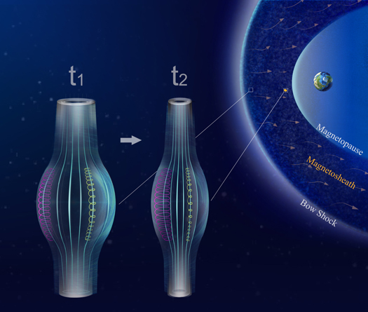
Figure 1. 3D sketch of the microscale magnetic cavity in the terrestrial magnetosheath as a magnetic bottle-like structure crossed by the spacecraft and an illustration of related particle dynamics. According to a particle sounding technique introduced recently for the same event, three spacecraft observation (MMS1 crossed the vicinity of structure's center while MMS3 and MMS4 traversed the outer part) showed a rounded cross-section of this magnetic cavity structure (Liu et al. 2019). The fact that enhanced phase space density (PSD) close to 90 degrees in the pitch angle distributions shown in Figures 2(e)–(i) are in agreement with the calculated loss cone (dashed lines) between trapped and un-trapped particle orbits indicates the existence of two mirror points, which can form a magnetic bottle-like structure to trap electrons. This structure was generated near the bow shock (e.g., at t1), and then carried by the sheath plasma flow downstream toward the magnetopause, encountering a region of increasing magnetic and thermal pressures. Driven by the increased pressure, the magnetic structure shrinks in the perpendicular direction (evidence indicating structure shrinkage is shown in Figure 3), resulting in the energy change of trapped electrons by energy-dependent gyro-acceleration, i.e., higher energy electrons (represented by a red spiral line within magnetic structure) accelerate while lower energy electrons (represented by yellow spiral line) decelerate. This acceleration gives rise to a distinct energy-dependent electron distribution feature at t2, as shown in Figures 2(b)–(i) observed by MMS in the vicinity of the magnetopause.
Download figure:
Standard image High-resolution image2. Results
In Figures 2(b)–(i), we plot the pitch angle distributions for electrons during the event reported by Yao et al. (2017), which has a spatial scale of about 20 km (the gyro-radii of the 40, 200, 400 eV electrons are about 1.3, 2.8, 4.0 km, respectively, for a minimum magnetic field of 17 nT) at 14:59:34 UT on 2015 October 23. In comparison with the ambient plasma outside of the structure, the phase space density (PSD) for electrons inside the magnetic cavity structure increases remarkably for pitch angles near 90° and energies higher than 90 eV, while the PSD decreases for energies below 70 eV. This event is one example of several such events that have been found in the magnetosheath, and is used as a typical subject of study, upon which we base our finding of a non-adiabatic acceleration process for electrons in microscale magnetic cavity structures.

Figure 2. Observed and simulated electron pitch angle distributions (PADs) in the magnetic cavity. (a)–(i) A magnetic cavity structure event observed by MMS1 at 14:59:34 UT on 2015 October 23: (a) the magnetic field intensity (Btot) along the satellite trajectory, with a magnetic cavity observed over a ∼0.3 s duration, indicating a spatial size of ∼20 km, and (b)–(i) electron PADs in different energy ranges, showing significant enhancement at higher energy bands (>∼90 eV) and a clear reduction at lower energy bands (<∼70 eV). The dashed curves in each plot of (b)–(i) indicate the critical trapped angles of  , where B is the magnetic field intensity and
  is the maximum at the mirror point. The higher energy electron PSD enhancement around 90° pitch angle fits well with critical trapped angles, suggesting a magnetic bottle-like structure trapping electrons. (j)–(r) The simulation results showing the PSD of test particles arriving at a virtual detector with bins in energy and pitch angle corresponding to those of the observation, as a function of spatial location across the magnetic structure, after an elapsed time of
  : (j) the magnetic field intensity along a trajectory crossing the center of the structure and (k)–(r) the simulated PADs at
  for electrons in different energy bands, for which the initial distributions was set according to the observed background with a linear interpolation being applied in a range of 0°–180° and 10–500 eV, respectively.
Download figure:
Standard image High-resolution imageA 3D illustration of the inferred magnetic structure based on observations is shown in Figure 1, and demonstrates that the topology forms a magnetic bottle-like structure to trap charged particles in the magnetosheath. Before being observed, the structure was generated upstream closer to the bow shock, and was then carried by the sheath plasma flow. It thus propagated downstream toward the vicinity of the magnetopause (Yao et al. 2017) where the background magnetic and thermal pressures are stronger than upstream (Shi et al. 2009). This causes a pressure difference between the inside and outside of the structure, which can be seen in Figure 5(g) of Liu et al. (2019). Compressed by this increasing external pressure during its propagation with the plasma flow, the structure in the magnetosheath is likely to gradually shrink in the perpendicular direction.
Because of the practical difficulties of detecting the spatio-temporal evolution of extremely small magnetic structures, most previous studies (Huang et al. 2017b; Yao et al. 2018a, 2018b) have been forced to focus on static structures, which has limited our understanding of critical particle behaviors in evolving electromagnetic environments. Here, we use an observed temporal variation of the magnetic field via a particle sounding technique (Liu et al. 2019) as the satellite traverses the magnetic structure, to infer its evolution with time. Figure 3 shows that the cross-sectional radius of the magnetic structure deduced from observations at its front exceeds that at its rear. Moreover, the value of Btot near the center at the rear is less than the value at the front. This indicates a shrinkage in cross-sectional radius and reduction in central magnetic field intensity with time. These results are also consistent with previously observed magnetic cavity structures at different stages of evolution (Yao et al. 2017) and theoretical predication (Li et al. 2016), which demonstrate that the level of reduction in their magnetic field strength is inversely related to their size. A shrinking rate of approximately 4 km s−1 for the outer boundary of the structure is indicated in Figure 3(d).
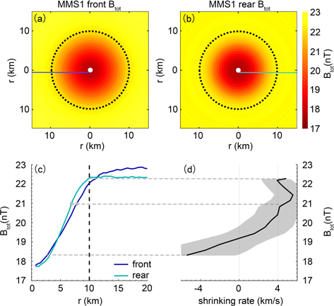
Figure 3. Magnetic field intensity from MMS1 implying a shrinking scenario. After determining the center of the structure (uncertainty ±0.2 km) via a particle sounding technique (Liu et al. 2019), the MMS1 observations of the magnetic field strength (Btot) are divided into front and rear parts as the satellite transits the structure. (a)–(b) The reconstructed 2D configurations based on rotational symmetry of the structure using the front and rear Btot, respectively, where r represents the radial distance to the center of the structure. It is clear that the outer boundary derived from the rear observation in (b) is slightly smaller than that derived from the front observation, indicating a shrinking structure. (c) The front and the rear Btot plotted as functions of the radial distance r. Dotted circles in (a) and (b) and a dashed line in (c) denote r = 10 km. Compared with the front part, the rear part of Btot is weaker near center and stronger in the outer region. (d) The estimated shrinking rate  , where
  is the difference in radial distance between the rear and front data at the same Btot, and
  is the corresponding duration for the satellite traversal. A shrinking rate is then evaluated approximately ∼4 km s−1 for the outer boundary of the structure.
Download figure:
Standard image High-resolution imageTo investigate the electron motion within the structure, we propose a numerical magnetic field model (see details in Appendix A and Figure A1) with an evolving magnetic cavity that reproduces the observed characteristics of the magnetic intensity decrease near the structure center as it shrinks. Based on this model, we show in Figure 4(a) the magnetic field magnitude Btot along a trajectory in the equatorial cross section through the center of the structure, indicated by the yellow dashed cut in Figure 4(d). As the structure shrinks with the observed rate of ∼4 km s−1, Btot in Figure 4(a) changes across the structure from the blue to the cyan curve. Its temporal variation per gyro-period is then calculated and shown in Figure 4(b). By Faraday's law, an azimuthal electric field (Eφ) with its direction in the center opposite to that in the outer region (Figure 4(c)) is induced. Due to the rotational symmetry of the magnetic structure, we can derive the distribution of the induced electric field in the equatorial plane (Figure 4(d)) from Figure 4(c). It is found that the direction of the electric field (blue curves with arrows) is counterclockwise (right-handed) near center and clockwise (left-handed) in the outer region.
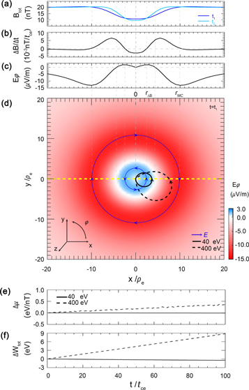
Figure 4. Schematic diagram of the non-adiabatic acceleration process in the magnetic cavity structure. (a) The magnetic field intensity at two typical moments t1 and t2( ,
,  , thus the shrinking rate v ≈4 km s−1). (b) Variation rate of the magnetic field. (c) The induced electric field calculated from the magnetic field variation (calculation method given in Appendix A). Note that the estimated maximum electric field is only ∼14 μV/m (0.014 mV m−1), which is too weak to be detected by the MMS electric field instrument (which has an accuracy of 0.3 mV m−1 (Lindqvist et al. 2014). (d) The induced electric field in the equatorial plane of the structure, and trajectories of two representative electrons (40 eV and 400 eV energies). (e)–(f) Test particle simulation results of two representative electrons, showing the time variation over an interval of 100 tce of the magnetic moment (e) and the energy (f). Violation of the adiabatic condition and energy gain for the 400 eV electron together with the magnetic moment conservation and energy loss of the 40 eV electron are shown.
Download figure:
Standard image High-resolution imageWe then use test particle simulations to investigate and validate the electron energization caused by such an induced electric field due to the structure shrinkage. In the simulation, the time and length scales are normalized by typical values for the electron gyro-period ( ) and the gyroradius (ρe = 1 km), i.e.,
  , and
, and  . Two 90° pitch-angle electrons initiated at the center are investigated, one with a lower energy (40 eV) and the other with a higher energy (400 eV). The trajectories of the two electrons over a gyro-period are highlighted as black solid (for 40 eV) and dashed (for 400 eV) loops in Figure 4(d). The electron gyration is counterclockwise, thus in line with the electric field near the center but opposite to it in the outer region. The lower energy electron only gyrates in the inner region, while the higher energy electron crosses the inner region to reach the outer region. As a consequence, higher energy electrons are accelerated while lower energy electrons are decelerated inside the shrinking magnetic cavity structure (see Appendix B for a theoretical derivation of this result). The results can be clearly seen from the variation of the magnetic moments △μ (where
  , and the angle bracket denotes averaging over one gyro-period) in Figure 4(e) and the variation of the total energy (
 ) in Figure 4(f) after 100 tce. For the 40 eV electron, though an energy loss is indicated by dWtot < 0 (solid line), the magnetic moment does not change significantly. The approximate conservation of μ indicates that the deceleration is quasi-adiabatic and likely due to the betatron effect. In contrast, the magnetic moment increases for the 400 eV electron (dashed line) along with its energy, indicating a non-adiabatic acceleration process. The simulation therefore reveals that the shrinking magnetic cavity structure naturally provides an energy-dependent acceleration process.
A simulation containing fifty million electrons distributed over various positions with different pitch angles and energies is further carried out to study the effect of the energy-dependent acceleration process on the electron distribution. The distribution of the pitch angle and energy are initialized by the observed background in Figures 2(b)–(i), while a linear interpolation is applied in a range of 0°–180° and 10–500 eV, respectively, and normalized by a typical value of PSD  . The density is approximately uniform in the simulation domain (
 ), with an open outer boundary condition. After the magnetic cavity structure has shrunk at
  , as shown in the right column of Figure 2, the PSDs of the trapped (close to 90° pitch angle) electrons are substantially increased at high energy in comparison with the ambient plasma outside of the structure, while the PSDs of lower energy electrons are decreased. The simulation results (right column of Figure 2 are clearly in qualitative agreement with the observations (left column of Figure 2).
3. Summary and Discussion
In this study, we have identified an extremely small magnetic bottle-like cavity structure using MMS observations and determined based on the observations that it is shrinking in size with time. We have found that a new, non-adiabatic acceleration process, which we denote "non-adiabatic collapse acceleration," occurs within this structure, and is explained by test particle simulation. This non-adiabatic acceleration can provide an alternative mechanism for energy transfer and particle acceleration when the typical spatial scales of the field are comparable to the gyromotion of the particles. Because of the propagation of magnetic cavities toward the vicinity of the magnetopause carried by the sheath plasma flow, the acceleration process is likely to be irreversible. In this type of microscale environment, electrons trapped in the magnetic cavity configuration can be repeatedly accelerated in the structure to make the acceleration process additive, until they eventually become un-trapped. Since the magnetic structure is shrinking, the segment of the electron population that is non-adiabatically accelerated changes in energy, with the upper and lower bounds lowering in energy as the structure decreases in size. Hence, magnetic structures such as these could play a role in the heating of electrons across a wide range of the energy spectrum throughout their lifetime. Although the energy gain per gyro-period for this particular case investigated appears not as striking as many other processes, the particle distribution has been clearly altered. Plasmoids that have been heated by this process may collectively affect conditions downstream, and alter conditions in the magnetosheath and even further in the magnetosphere.
In general, microscale structures have great relevance across a number of branches in plasma physics, including space, astrophysical, and laboratory plasmas. Collectively, these structures may substantially impact macroscopic plasma processes, such as energy dissipation and particle acceleration/heating occurring in magnetosheath-like environments. These universal environments exist behind shocks in the solar wind or in front of planetary magnetospheres, and are also seen in an interstellar medium with compressible fluctuations (Armstrong et al. 1981; Zhuravleva et al. 2014). In particular, particle heating/acceleration commonly occurs within turbulent plasmas (Matthaeus & Velli 2011; Alexandrova et al. 2013; Chen 2016), which tend to cascade energy down to the small scales, of order the electron gyro-scale (see the turbulent environment of this event and more discussions in Appendix C and Figure C1). Since in the magnetosheath such kinds of structures are widespread, the cumulative effect on particle acceleration can be expected to be substantial. Furthermore, considering broader regions such as astrophysical environments, the magnetosheath and other compressive fluctuating environments that exist behind interstellar shocks or around many astrophysical bodies are known to have more extreme electromagnetic conditions (Mckee & Ostriker 2007; Slavin et al. 2008; Zhuravleva et al. 2014; Hadid et al. 2015). In such cases the magnetic field and thus the induced electric fields should be much larger than those in the Earth's magnetosheath, and should result in a more significant acceleration rate. Thus the effect of this process on the particle distribution may provide some perspectives for particle acceleration/energy dissipation through magnetic bottle-like structures in astrophysical and laboratory plasmas, which can be tested in future studies.
We are very grateful to R. Erdélyi, W. J. Sun, X. Z. Zhou, X. C. Guo, M. G. Kivelson, K. K. Khurana, and D. Verscharen for their suggestions on this work. We greatly appreciate the instrumental teams of MMS for providing magnetic field and plasma data for our observation studies. We also thank the International Space Science Institute (ISSI) for their support. This work is supported by the National Natural Science Foundation of China (grant Nos. 41774153, 41674165, 41731068, and 41961130382), Young Scholar Plan of Shandong University at Weihai (2017WHWLJH08), the Specialized Research Fund for State Key Laboratories, the fund of Shandong Provincial Key Laboratory of Optical Astronomy and Solar-Terrestrial Environment, National Key Research and Development Program of China from MOST (2016YFB0501503), Newton Advanced Fellowship (R1\191047). Z.Y. is a Marie-Curie COFUND postdoctoral fellow at the University of Liege, co-funded by the European Union. All observation data used are available from MMS Science Data Center (https://lasp.colorado.edu/mms/sdc/public/). The simulation code is available from the corresponding author upon reasonable request.
Appendix A: The Magnetic Field Model
The magnetic field is modeled by a magnetic field generated by ring current superimposed upon a homogeneous background magnetic field. In a cylindrical coordinate system ( , we select the background field direction as the z-axis. The current density is then calculated from the following model equations:


where the variables jp and rp are the peak value of the current density at z and its radial position, with  and
and  at z = 0. The parameter d0 denotes the decay rate of rp along the z-direction.
With the current density distribution, the magnetic vector potential  can be solved from the following equation:

where c is the speed of light. Then the magnetic field  and electric field
  can be calculated by
where  is the background magnetic field, Φ is the electric potential (here
  ).
).
According to observations of microscale magnetic cavity structures, as the structure shrinks, the magnetic field intensity decreases near the central axis (the symmetric axis of magnetic cavity structure), i.e., the magnetic field is reduced at r = 0 but increased for large r, i.e.,

where rMC is the typical size of the magnetic cavity structure and  is the critical radius where
  .
.
Here, we construct a shrinking magnetic cavity structure as follows. The parameters  and
and  are set as the following functions of time t in the model:
where the shrinking rates  . In addition, we set
  for Equation (A2). The background field
  is set to 20 nT along the z-direction. The result using this parameter set is shown in Figure A1. The length of the magnetic cavity structure is
  ; the initial radius of the magnetic cavity structure is
  and decreases to 5ρe over a time interval of at 2000 tce. During this time, the magnetic field intensity in the center is decreased from 15 to 9 nT.

Figure A1. Model of the shrinking magnetic cavity structure. (a) The magnetic field intensity along a trajectory crossing the center of the structure, i.e., the yellow dashed line in the equatorial plane (z = 0), at  and
and  , respectively. (b) The distribution of magnetic field intensity on y = 0 plane at
  .
.
Download figure:
Standard image High-resolution imageHere, the induced electric field can be also understood as follows. As the structure shrinks, the magnetic field intensity decreases ( ) near the central region of the structure and increases in the edge region (
 ), as shown in Figure 4(b). In cylindrical coordinates, Faraday's Law gives
  . Therefore, we integrate numerically using the boundary condition Eφ = 0 at r = 0 with given
  to obtain Eφ as shown in Figure 4(c). In our simulation, we solved Equation (A4), another form of Faraday's Law, to obtain the same result.
Appendix B: The Acceleration Process
In the shrinking structure, the temporally varying magnetic field leads to an induced electric field, which does work on the charged particles,  . The change in energy over one gyro-period is
where q is the charge of the particle,  is a line element of the gyration orbit l, E is the electric field, and S is the surface enclosed by the gyration orbit. If the temporal and spatial variations of the field are slow enough, the variation of the perpendicular energy
  over the gyro-period can be simplified as
  , where μ and
  are the magnetic moment of the charged particle and the intensity variation of magnetic field, respectively. However, in a microscale magnetic cavity structure where the gradient scale is comparable to charged particle gyroradius, the condition of the magnetic field homogeneity (
 ) is no longer valid. Thus the magnetic moment is not conserved and the acceleration should be regarded as a non-adiabatic process. From Equations (A5) and (B1), the energy gain for an electron trapped in a magnetic cavity structure and crossing the center can be written as
where  is the gyration diameter,
  is the critical radius for the energy gain
  when
when  . Electrons with a small gyroradius are trapped in the center, where the magnetic field decreases (corresponding to the first case of Equation (B2b)), and will lose energy. However, for electrons with a large gyroradius comparable to the structure size (corresponding to the third case of Equation (B2b)), an energy gain can be achieved. Since
  , the temporally varying field inside the magnetic cavity structure can therefore decelerate the lower energy electrons and accelerate the higher energy electrons.
Appendix C: The Turbulent Environment of the Structure
Turbulent magnetized plasmas are common in sheath of celestial objects immersed in plasma flow (Hadid et al. 2015; Huang et al. 2017a). Compared to the extensively studied turbulence in solar wind (Velli et al. 1989; Verdini et al. 2012; Woodham et al. 2018), the turbulence in the magnetosheath shows distinct differences, for example, the fluctuations have a significant compressive component compared to the Alfvenic component (Alexandrova et al. 2013; Huang et al. 2017a, 2017b; Zhu et al. 2019). Furthermore, according to the recent observations, some coherent structures such as mirror modes and electron vortices are frequently detected in this turbulent magnetosheath and inside of the magnetosphere. These structures are regarded as products of the turbulent cascade and possibly associated with enhanced dissipation (Sahraoui et al. 2004, 2006; Huang et al. 2017b). Numerical simulations of decaying turbulence also show the presence of turbulent structures (Haynes et al. 2015; Roytershteyn et al. 2015).
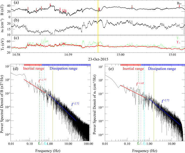
We further analyze the fluctuations of the background magnetic environment and the corresponding power spectral density during an interval of 100 s before and after this event, as shown in Figure C1. The disordered magnetic field and electron number density fluctuations, as well as their power-law spectra, are consistent with the following classical features of plasma turbulence. 1. The power spectral density of the magnetic field (or electron number density) fluctuations shows two power-law slopes, i.e., ∼−5/3 at MHD scale and ∼−2.7 at sub-ion scales, which are consistent with previous studies on turbulence in the magnetosheath (Sahraoui et al. 2006; Huang et al. 2017a, 2017b). 2. A clear break of the slope is revealed at about Taylor-shifted ion inertial length fdi. In addition, we can find that the scale of this structure is in the dissipation range of turbulence and the perpendicular electron temperature in the structure is clearly higher than that outside. Thus, this magnetic cavity should be referred to as a structure embedded in the turbulent plasma, and this work may also provide a possible mechanism to reveal the outstanding question of how energy dissipated by turbulent structures (Chen 2016). The observed structure may not be directly generated by the cascade of the turbulence, but it can still take energy from the fluctuations at scales in the order of the structure size, which will then act as a route of dissipation of the turbulence.
Figure C1. Background environments of the event used in this Letter. (a)–(c) Magnetic field intensity, electron number density, and electron temperature (parallel and perpendicular temperature are in green and red, respectively) from 14:57:54 UT to 15:01:14 UT on 2015 October 23. The magnetic cavity structure analyzed in this Letter is marked by the yellow shaded region, and the red arrows denote some other structures with decreased magnetic field magnitude and roughly similar electron PADs. (d)–(e) The power spectral density of the magnetic field fluctuations and electron number density fluctuations during the time interval shown in panel a. The fitted power laws within two frequency ranges marked by red and blue show the spectral indices of the inertial and dissipation ranges. The vertical dashed lines in 0.33, 0.41, and 0.58 Hz indicate the scale of the Taylor-shifted ion gyroradius  (green), ion gyro-frequency fci (gray), and Taylor-shifted ion inertial length fdi (cyan), respectively, for the average condition where magnetic field, flow speed, number density, and ion temperature are 27 nT. 198 km s−1, 18 cm−3, and 330 eV, respectively. The solid yellow line at 1.58 Hz marks the scale of this magnetic cavity structure (
 ).
).
Download figure:
Standard image High-resolution image