


1. Introduction
Due to their sensitivity to changes in air temperature and precipitation, glaciers have been recognised as an Essential Climate Variable (ECV) (GCOS, 2016). In line with most glacierised mountain ranges, glaciers of Chile have been generally retreating and thinning since the middle of the 20th century (Le Quesne and others, Reference Le Quesne, Acuña, Boninsegna, Rivera and Barichivich2009; Malmros and others, Reference Malmros, Mernild, Wilson, Fensholt and Yde2016; Farías-Barahona and others, Reference Farías-Barahona2019). As in other mountainous areas in the world, this behaviour has raised concerns regarding the sustainability of water resources, particularly during dry seasons and periods of drought (e.g. Ayala and others, Reference Ayala2016). In the case of the Maipo River, which flows through the heavily populated capital city of Santiago in the Metropolitan Region in Chile (7 million inhabitants), glaciers have been identified as a key water resource particularly when melt contributions from seasonal snow cover are exhausted (Peña and Nazarala, Reference Peña and Nazarala1987; Mernild and others, Reference Mernild2015; Ayala and others, Reference Ayala2016). Modelled studies of basin-wide glacier runoff contributions to the upper Maipo River since 2000 indicate an increasing trend of ice melt contribution during the past decade (Burger and others, Reference Burger2019).
In recent years, a large number of glaciological and climatological studies in the Central Andes have improved our knowledge of glacier–climate interactions in this region (e.g. Ragettli and others, Reference Ragettli, Cortés, McPhee and Pellicciotti2013; Pellicciotti and others, Reference Pellicciotti, Ragettli, Carenzo and McPhee2014; Ayala and others, Reference Ayala2016; Masiokas and others, Reference Masiokas2016; Bravo and others, Reference Bravo, Loriaux, Rivera and Brock2017; Braun and others, Reference Braun2019; Burger and others, Reference Burger2019; Farías-Barahona and others, Reference Farías-Barahona2019, Reference Farías-Barahona2020; Schaefer and others, Reference Schaefer, Fonseca, Farías-Barahona and Casassa2020; Ayala and others, Reference Ayala2020). However, multi-temporal analyses of glacier fluctuations, in particular, have focused mainly on changes in glacier length and area (e.g. Rivera and others, Reference Rivera, Acuña and Lange2000; Malmros and others, Reference Malmros, Mernild, Wilson, Fensholt and Yde2016) and there are comparatively few long-term mass-balance records, although these provide the most valuable information concerning glacier response to climate change (Escobar and others, Reference Escobar, Casassa and Pozo1995; Leiva and others, Reference Leiva, Cabrera and Lenzano2007). In the Central Andes of Chile, for example, the Echaurren Norte Glacier is the longest glacier mass-balance record (1975 to present) using the glaciological method (Escobar and others, Reference Escobar, Casassa and Pozo1995; Masiokas and other, Reference Masiokas2016; Farías-Barahona and others, Reference Farías-Barahona2019, Reference Farías-Barahona2020). However, this glacier sample represents only a small fraction of the glaciers that exist in the entire Chilean and Argentinean Andes (Barcaza and others, Reference Barcaza2017; RGI Consortium, 2017). In light of this knowledge gap, recent studies using multi-temporal satellite- and ground-based analyses of glacier elevation (Malmros and others, Reference Malmros, Mernild, Wilson, Fensholt and Yde2016; Braun and others, Reference Braun2019; Dussaillant and others, Reference Dussaillant2019; Farías-Barahona and others, Reference Farías-Barahona2019) and ice velocity change (Wilson and others, Reference Wilson, Mernild, Malmros, Bravo and Carrión2016) have provided important additional data sources and have proved to be useful surrogates for assessing glacier fluctuations in the Central Andes of Chile.
Here, we provide a detailed and multi-temporal study of geometric changes in El Morado Glacier and its adjacent proglacial lake using an ensemble of topographic information obtained from archival aerial and terrestrial photography, multispectral satellite imagery, aerial and terrestrial Light Detecting and Ranging (LiDAR) surveys data and satellite Synthetic Aperture Radar (SAR) data, which was not previously included in Farias-Barahona and others (Reference Farías-Barahona2020). Through analysis of these remotely sensed datasets, we quantify both ice area and surface elevation changes for the entire glacier (1955–2019) and the glacier tongue (1932–2019).
Particular focus was given to the El Morado Glacier calving front, where a proglacial lake has been progressively increasing in size as a consequence of glacier retreat. The availability of the topographic information described together with bathymetric survey data obtained during a field campaign in 2017 has allowed us to conduct an assessment of the evolution and the volume of water storage in this lake, the first of its kind in the Central Andes. Finally, by combining different sources of climatological data, we estimate annual surface mass balance using a minimal glacial mass-balance model for the El Morado Glacier between the hydrological years 1979/1980 and 2015/2016. Such information allowed for an assessment of the sensitivity of this particular glacier to climate fluctuations.
2. Study area
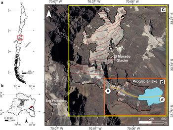
The El Morado Glacier (33°44′42.40″S, 70° 3′49.36″W, 3250 to 4500 m a.s.l.) is located in the El Volcan sub-basin of the Maipo River basin (Fig. 1). The Maipo River basin is one of the most glacierised areas of Central Andes and provides fresh water to Santiago, the Chilean capital city. El Morado Glacier is a south-east facing mountain glacier with an area of 1.05 km2 (2015), and is made up of three bodies of ice, with its partially debris-covered tongue being supplied by ice from accumulation areas located on the southern and south-western flanks of the ‘El Mirador del Morado’ mountain. Each of these ice bodies is connected by steep-sided icefalls, the largest of which supplies the glacier tongue (3250 and 3650 m a.s.l.), which the glacier now actively calves into its adjacent proglacial lake (Fig. 1c).

Fig. 1. Location (a) and spatial extent (b) of the Maipo River basin, central Chile. The Volcan sub-basin is highlighted within (b) along with the location of El Morado Glacier (red dot). The spatial extent of the glacier elevation and mass changes presented for the entire glacier and the glacier tongue is indicated in (c) and (d), respectively. The longitudinal profile A-A', which covers the glacier tongue and its adjacent proglacial lake, is shown in Figure 9.
In the Central Andes of Chile (31–35°S), the climate is classified as Mediterranean in type and is under the influence of the south-east Pacific anticyclone year-round (Garreaud, Reference Garreaud2013). Precipitation in this region is concentrated in the austral winter (June to September), generally falling as snow above altitudes of 2000 m, with glacier ablation generally being restricted to the summer season, which in comparison tends to be dry and warm.
Annual precipitation in the region is highly variable with marked interannual variability due to the El Niño Southern Oscillation (ENSO). However, since the 1980s, a reduction in total precipitation has been observed in coastal regions (Quintana and Aceituno, Reference Quintana and Aceituno2012). More recently, multi-temporal analyses of MODIS satellite imagery indicate that snow cover extent and duration across the central Chilean and Argentinean Andes have reduced by an average of ~13% and ~43 d between 2000 and 2016, respectively (Malmros and others, Reference Malmros, Mernild, Wilson, Tagesson and Fensholt2018). Since 2010, central Chile has also been affected by a severe drought, coined as a ‘mega-drought’ (Garreaud and others, Reference Garreaud2017, Reference Garreaud2019). Drought events are not uncommon in the Maipo River basin, but recent analyses suggest that their frequency and duration may have increased since the 1950s (Gonzalez-Reyes and others, Reference González-Reyes2017). On the other hand, recent studies show that the annual average temperature in the Upper Maipo has increased, mostly explained by spring and autumn warming (Burger and others, Reference Burger, Brock and Montecinos2018).
3. Data and methods
3.1 Quantifying glacier and lake area changes from satellite images and aerial photographs
To quantify areal changes in El Morado Glacier and its adjacent proglacial lake, satellite images and aerial photographs were orthorectified and geo-referenced and manually digitised (Table 1). The 1955 photogrammetric survey data were provided by the Chilean Military Geographical Institute (IGM) and represents the oldest large-scale geospatial information source for the glacier. Aerial photographs from 1983 by Chile-80 and 1996 by GEOTEC were obtained from the Chilean Air Force's Aero-photogrammetric Service (SAF). Each of these aerial photographs (1955, 1983 and 1996) was photogrammetrically scanned at a resolution of 1200 DPI prior to processing. The 1967 declassified stereo Corona KH-4A satellite imagery was acquired in digital format from the US Geological Survey (USGS). Additionally, several Landsat Thematic Mapper (TM), Operational Land Imager (OLI) and Google Earth images were also used, this imagery having been captured during the ablation season between 2000 and 2018. PlanetScope data (Planet Team, Reference Planet Team2018) with a pixel resolution of 3 m were acquired for 2019 through the Planet Labs Research and Education Initiative.
Table 1. Dataset used to map glacier area, frontal and proglacial lake change

Once orthorectified and geo-referenced, the manual digitisation of glacier and lake outlines from the satellite/aerial imagery was performed using standard procedures (Table 1). For Landsat images, we used the approach outlined by Paul and others (Reference Paul, Kääb, Maisch, Kellenberger and Haeberli2002). To improve consistency and accuracy of cross-comparisons, all glacier/lake outlines were digitised by the same expert user, with high-resolution satellite (SPOT 6: 2015) and aerial drone imagery (DJI Phantom 4: 2017) providing a detailed topographic reference point. The information provided by the satellite/aerial imagery was supplemented further by information obtained from mountaineering reports of the first German mountaineering expedition to El Morado Glacier in March 1932, led by Albrecht Maaß (DAV – Deutscher Andenverein, 1932). Of particular importance, photographs taken during this expedition were photo-interpreted, allowing coarse estimations of ice elevation change between 1932 and 2018. Field photographs acquired by the authors between 2003 and 2019 were also used to aid the photo-interpretation process. For the accuracy of the manual glacier/lake delineation process (δ A), we assumed an error of ±1-pixel size (n) (Williams and others, Reference Williams, Hall, Sigurosson and Chien1997). This delineation error was then multiplied by the perimeter length (pL) of the glacier/lake feature being mapped (Loriaux and Casassa, Reference Loriaux and Casassa2013; Casassa and others, Reference Casassa, Rodríguez, Loriaux, Kargel, Leonard, Bishop, Kääb and Raup2014).
3.2 Extracting DEMs from aerial imagery using Structure from Motion techniques
In order to extract DEMs from the HYCON (1955), Chile-80 (1983) and GEOTEC (1996) aerial imagery, Structure from Motion (SfM) techniques were applied. The SfM photogrammetric approach has become a common technique to derive 3D topographic data from overlapping image sequences (Westoby and others, Reference Westoby, Brasington, Glasser, Hambrey and Reynolds2012; Smith and others, Reference Smith, Carrivick and Quincey2016) and has reliably produced DEMs for the quantification of river-floodplain morphological changes (Bakker and Lane, Reference Bakker and Lane2016; Wilson and others, Reference Wilson2019), the estimation of glacier mass balance (Mölg and Bolch, Reference Mölg and Bolch2017), and the monitoring of rock glaciers (Vivero and Lambiel, Reference Vivero and Lambiel2019). In this case, the 1955, 1983 and 1996 digital aerial photography was processed using SfM algorithms embedded in the PIX4dmapper Pro software package (version 4.1). This process was aided by GCPs collected from stable non-glacier locations visible in the terrestrial laser scanning (TLS) and airborne LiDAR surveys. Based on these GCPs, the SfM workflow in Pix4D executes an iterative routine of block bundle adjustments (BBA), camera self-calibration and exterior parameter adjustments (Table 2). Subsequently, a coarse 3D point cloud is created from the extraction of numerous image tie points, and further multi-view stereo (MVS) methods are applied to derive a denser 3D point cloud (see Smith and others, Reference Smith, Carrivick and Quincey2016 for details). The resulting dense 3D point clouds (average 1–2 points per m2) were filtered for erroneous points using a static outlier removal tool available in Cloud Compare version 2.10 software (Girardeau-Montaut, Reference Girardeau-Montaut2019) and gridded at 1 m resolution using a triangulated irregular network method. The accuracy of this DEM generation process in comparison to the GCP observations is indicated in Table 2 (RMSE).
Table 2. SfM block bundle adjustment results from the different aerial surveys. The RMSE indicates how well the resulting 3D models fitted observations (GCPs)

3.3 TLS and airborne LiDAR and GNSS data
Four LiDAR scans of the glacier front were obtained for the years 2015, 2018 and 2019 (2 scans) using a REIGL VZ-6000 long-range TLS (Table 3). The TLS instrument obtains ranging measurements by actively transmitting short pulses of electromagnetic radiation towards a target object and then recording its return. Distances between the sensor and targets are then calculated using time-of-flight principles. For each of the observation periods, the glacier front was surveyed from two overlapping stable-ground scan locations. To obtain the absolute position of each LiDAR measurement location, two overlapping stable-ground scanning locations were used, measured using a mounted double-frequency GNSS receiver. For all LiDAR measurements, we obtained a horizontal and vertical accuracy of a few centimetres.
Table 3. Digital elevation models (DEMs) generated for the El Morado Glacier front

To enable comparisons, the January 2019 scan was subsequently used to co-register the other three TLS point clouds in Reigl RiScan® software using point-to-point feature matching and a subsequent iterative closest point algorithm of stable bedrock locations (RIEGL, 2015; Xu and others, Reference Xu2017). The average alignment error of the point cloud co-registration between each scan period was calculated as ~0.04 m. Co-registered point clouds were subsequently interpolated using the kriging method and exported in raster format with a horizontal resolution of 0.5 m and in the UTM 19S coordinate format. Assuming uncorrelated errors, the propagated error of the TLS differencing from GPS, point cloud and raster error sources was estimated as ±0.20 m (stable rock).
Additionally, a DEM covering the entire glacier was made available by the Water Directorate of Chile (DGA) (hereafter DGA-2015 DEM). This DEM was generated from SPOT imagery captured on 30 January 2015 using stable ground control points obtained from an Airborne LiDAR campaign also carried out in the summer of 2015 (DGA, 2015).
3.4 SRTM and TanDEM-X
The Shuttle Radar Topography Mission (SRTM) acquired near-global bi-static C-band Interferometric Synthetic Aperture Radar (InSAR) data between 11 and 22 February 2000 (Farr and others, Reference Farr2007). The SRTM-C DEM is available in a gap-filled 1 arcsec resolution. However, the original SRTM-C DEM covers just the tongue of El Morado Glacier (Farías-Barahona and others, Reference Farías-Barahona2020).
TerraSAR-X and TanDEM-X (TDX) is an ongoing satellite constellation launched by the German Aerospace Center (DLR) that has been acquiring bi-static X-band InSAR data since 2010 (Krieger and others, Reference Krieger2007). Here, the TDX scenes used were processed following methods described by Braun and others (Reference Braun2019) and Farías-Barahona and others (Reference Farías-Barahona2019), utilising tools available within GAMMA software and elevation reference data from the SRTM-C DEM. The topographic phase of the SRTM-C DEM was simulated using TanDEM-X interferometric parameters to obtain the double-difference interferogram. The noise in the interferogram was suppressed using the Goldstein filter (Goldstein and others, Reference Goldstein and Werner1998). Areas degraded due to shadow and water bodies were masked before unwrapping the differential phase using a minimum cost flow (Costantini and others, Reference Costantini1998) algorithm. We converted the unwrapped phase into a differential height or TanDEM-X DEM. Finally, the TDX DEM was post-processed using an approach detailed by Braun and others (Reference Braun2019).
3.5 DEM correction, geodetic mass-balance calculation and uncertainties
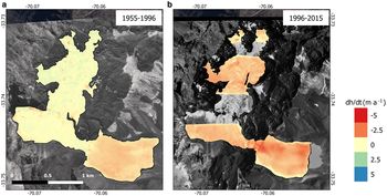
In lieu of detailed field measurements, geodetic mass-balance calculations, whereby remotely sensed DEMs acquired over a glacier surface are differenced to estimate ice elevation and volume changes, provide an invaluable and indirect method of assessing glacier behaviour over varying time frames (e.g. Farías-Barahona and others, Reference Farías-Barahona2019). The DEMs used in this study are detailed in Tables 3 and 4. Prior to calculating the geodetic mass balance, these DEMs were firstly resampled before being co-registered (horizontally and vertically) using the approach outlined by Nuth and Kääb (Reference Nuth and Kääb2011). Overall, the DEM co-registration processes resulted in a good level of cross-alignment. However, the 1983 DEM exhibited a number of elevation errors in areas where the GCP distribution was limited and was subsequently excluded from the analysis. Elevation changes obtained from the DEM differencing procedure were converted to mass change assuming ice densities of 850 ± 60 kg m−3 (Huss, Reference Huss2013). The geodetic mass balance was calculated for the entire glacier area (see Fig. 1c) for the 1955–1996 and 1996–2015 observation periods.
Table 4. Digital elevation models (DEMs) generated for the El Morado Glacier (entire glacier area)

The level of uncertainty attributed to the geodetic mass-balance calculations conducted quantified through error propagation (Malz and others, Reference Malz2018; Braun and others, Reference Braun2019; Farías-Barahona and others, Reference Farías-Barahona2019). This process included uncertainties derived from the volume to mass conversion (δ ρ) (which correspond to 7% or ±60 kg m−3 – Huss, (Reference Huss2013)), errors quantified for stable non-glacier areas during the DEM differencing procedures (δΔh/Δt) (considering spatial auto-correlation) and error associated with the glacier outlines (δ A) (Section 3.1). Any potential uncertainty associated with radar signal penetration (in the case of SRTM and TanDEM-X) was not considered in this case because the surveyed area (the glacier tongue/ice cliff) included only ice.

The error derived from the DEM differencing (δ Δh/Δt) was obtained using the approach outlined by Rolstad and others (Reference Rolstad, Haug and Denby2009) (Eqn (2)), which has been applied in other similar glaciological studies that have used ASTER DEMs (e.g. Dussaillant and others, Reference Dussaillant2019), Hexagon images (Maurer and others, Reference Maurer, Schaefer, Rupper and Corley2019), TanDEM-X (Braun and others, Reference Braun2019) and terrestrial LiDAR (Fischer and others, Reference Fischer, Huss, Kummert and Hoelzle2016).

where A is the glacier area and A cor corresponds to the range over which errors in DEM differencing are spatially correlated, estimated as A cor = π × L 2, L corresponds to the correlation range (from 100 to 850 m), and σ Δh/Δt corresponds to the std dev. of errors in elevation changes, which is performed as area weighted calculated for each 5° slope bin over stable areas. For the 2015 Spot/LiDAR DEM (entire glacier), linear striping is evident in the upper parts of the glacier. Unfortunately, the original raw data for this the DEM was not available for re-processing. We compare our LiDAR TLS (2015) on stable ground and we were able to remove those strips and we calculate the elevation changes using the local hypsometric method. We have estimated an additional uncertainty of ±0.15 m a−1 for the 1996–2015 observation period.
3.6 Lake bathymetry and glacier tongue flotation
The bathymetry survey of the proglacial lake was conducted during a field visit on 11 February 2017 using a custom-built expanded polystyrene remote-controlled boat fitted with a 150 kHz thru-hull depth transducer connected to Actisense Dst-2 active depth sounder module. The control system for the sounder module included an ATMega 328 microcontroller, an uBlox NEO-6 GPS unit and an RFM69HW radio transceiver that was used during debugging. The boat itself was controlled manually using a standard 2.4 GHz radio system and water depth measurements were acquired every 3 s. Further specifications for the bathymetry boat are available in Wilson and others (Reference Wilson2019). Using the lake depth data acquired in the field, a 2 m grid bathymetry DEM was interpolated using the kriging method. The lake volume was calculated using the bathymetry DEM and the waterline with 0 m depth, which is derived from aerial photographs acquired on the same day as the bathymetry measurements (Section 3.1). This bathymetry and the topography data were used to estimate and determine how close the glacier tongue was to flotation during our study period, using the flotation thickness estimation (Benn and others, Reference Benn, Warren and Mottram2007; Boyce and others, Reference Boyce, Motyka and Truffer2007).
Regarding the bathymetry uncertainties, we estimated a depth uncertainty of ±1.2 m. This uncertainty was calculated using error propagation, considering errors related to the depth sounder equipment, uncertainty of the acoustic velocity due to water temperature (0.7% of the depth) (e.g. Haritashya and others, Reference Haritashya2018) and depth differences obtained from overlapping track lines.
3.7 Minimal surface mass-balance model
The mass balance of El Morado Glacier was reconstructed between the hydrological years 1979/1980 and 2015/2016 using climate data and the so-called minimal glacier mass-balance model approach (Marzeion and others, Reference Marzeion, Hofer, Jarosch, Kaser and Molg2012). This model was applied to reconstruct the annual mass balance for the Echaurren Norte Glacier, located 20 km north of the study area (Masiokas and others, Reference Masiokas2016). The model is defined in Eqn (3) as:

where MB is the annual specific mass balance, P i is the monthly precipitation and α is a scaling parameter for precipitation, T i is the mean monthly air temperature, T melt is the monthly mean temperature above which melt occurs and μ is the melt factor (in mm °C). The maximum operator ensures that melting occurs during the months with the mean air temperature above T melt. Due to the lack of ground-based mass-balance observations, we assume the same values by Masiokas and others (Reference Masiokas2016) for Echaurren Norte Glacier for the parameters α, μ and T melt (3.9 (α), 89 mm °C(μ) and 0 °C). The model requires as forcing, monthly data of air temperature and precipitation. These input data were taken from the CR2MET dataset (Alvarez-Garreton and others, Reference Alvarez-Garreton2018). The CR2MET is a new gridded climatology dataset available at daily and monthly time step with a grid size of 0.005° (~5 km). In the case of precipitation, the data was obtained using the ERA-Interim reanalysis and using transfer functions and statistical models that take account of the local topography and parametrisations estimated from observations. For air temperature, a grid was constructed again using the large-scale variables (ERA-Interim) as well as the local observations and topography. This grid also included remotely sensed air temperature estimations (MODIS-LST) (http://www.cr2.cl). CR2MET air temperature data were validated and corrected with on-glacier observations collected at San Francisco Glacier, which is located immediately west of El Morado Glacier on the same CR2MET gridpoint (Fig. S1). These observations measured on the surface of San Francisco Glacier were acquired by two Automatic Weather Stations, the first (AWS1) installed at 3806 m a.s.l. and the second (AWS2) installed at 3466 m asl. The AWS1 observations span the period from 1 December 2012 to 18 April 2013. The daily mean of these meteorological observations was used to transfer the CR2MET data to the 3806 m a.s.l. (Figs S2, S3). As the minimal glacier model requires the air temperature at the elevation of the front of the glacier, we used an environmental lapse rate of −0.0065 °C m−1 (Barry, Reference Barry2008), which is a shallower lapse rate that has been typically observed over the glaciers (e.g. Petersen and Pellicciotti, Reference Petersen and Pellicciotti2011; Shaw and others, Reference Shaw, Brock, Ayala, Rutter and Pellicciotti2017; Bravo and others, Reference Bravo2019). Due to the uncertainty in the lapse rates, we use a range that comprises between −0.0045 and −0.0085 °C m−1. The on-glacier observations ensure that the cooling effect observed over the glacier surface (e.g. Ragettli and others, Reference Ragettli, Cortés, McPhee and Pellicciotti2013; Ayala and others, Reference Ayala, Pellicciotti, Peleg and Burlando2017) is included in the correction.
Regarding precipitation, the CR2MET data include values and variability similar to the observations of El Yeso Embalse (2475 m a.s.l) weather station, located 8 km north of the glacier (Fig. S4). Considering the difference in elevation between Yeso Embalse and the front of El Morado Glacier, and the similarities in the amount of precipitation, the same value for the parameterα was used to compensate for the precipitation gradient as at Echaurren Norte Glacier by Masiokas and others (Reference Masiokas2016).
4. Results
4.1 Glacier area changes
Our results reveal a total ice-area loss of 0.61 ± 0.05 km2 between 1955 and 2019. This value represents a total area reduction of 40% for El Morado Glacier over the 64-year observation period (Fig. 2 and Table 5). Noticeable is the glacier area loss between 2015 and 2019, with a total of 0.15 km2 in 4 years. Figures 2d–k show the frontal changes observed for the glacier between 1955 and 2019. Overall, the glacier front retreated by 10.30 ± 1.74 m a−1 over the 64-year observation period. However, this retreat rate varies through time, with the glacier front going through periods of extensive retreat (e.g. 1955–1967; 1967–1986; 1996–2000) interspersed by periods of small changes (e.g. 1986–1996 and 2000–2010). However, the highest rates of retreat were observed between 2010 and 2019 (−37.50 ± 5.79 m a−1), peaking between 2013 and 2015 when the central section of the glacier front retreated by 150 ± 30 m.

Fig. 2. Area changes in the entire El Morado Glacier (a–d), and its glacier tongue (e–l) between 1955 and 2019. Orange glacier outline corresponds to the 1955 glacier area.
Table 5. Summary of the geodetic mass balances of the entire El Morado Glacier for the 1955-1996 and 1996-2015 observation periods (Fig. 1c)

We assumed a density scenario of 850 ± 60 kg m−3.
4.2 Glacier surface elevation and mass changes
Figures 3 and 4 show the glacier elevation change maps obtained for the entire glacier (Fig. 1c) and the glacier tongue (Fig. 1d). For the entire glacier, a mean geodetic mass balance of −0.39 ± 0.15 m w.e. a−1 was obtained between 1955 and 2015 (Figs 3a, b). The spatial pattern of change between 1955 and 1996 is quite heterogeneous. The upper part of the glacier (3650–4500 m a.s.l) shows positive values, while in the glacier tongue (3250–3650 m a.s.l), there are negative elevation changes. Between 1996 and 2015, the mass balance for the whole glacier is clearly negative (Table 5), highly influenced by the glacier tongue.

Fig. 3. Elevation change maps of the El Morado Glacier. (a) and (b) correspond to the periods 1955–1996 and 1996–2015, respectively.

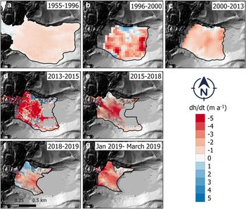
Fig. 4. (a–g) Glacier tongue elevation change for El Morado Glacier at seven periods between 1955 and 2019.
For the glacier tongue (Fig. 1d), a mean elevation change rate of −1.18 ± 0.22 m a−1 was observed between 1955 and 2019 (Figs 4a–g). Further details of the glacier elevation changes are presented in Table 6. In terms of temporal variability, the glacier front underwent the greatest changes between 2013 and 2019. During this period, the glacier front downwasted at a maximum rate of −4.10 ± 1.50 m a−1 between 2013 and 2015, followed by a rate of −2.63 ± 0.06 m a−1 between 2015 and 2018 (Table 6 and Fig. 4). For the latter period, thinning was particularly pronounced at the central portions of the ice cliff that feeds the glacier tongue, with values of up to 30 m being observed. The 2019 ablation season saw further losses with the glacier tongue thinning by an average of −2.68 ± 0.20 m a−1 between January and March alone. These losses contributed to a total thinning of 3.87 m between 2018 and 2019. The elevation changes derived from photographs taken by Albrecht Maaß in March 1932 are shown in Figure 5. Through photo-interpretation, assuming this elevation change as equivalent to the entire glacier tongue, we estimated an ice elevation change of −0.50 m a−1 for the 1932 to 1955 observation period for the glacier tongue. Finally, total ice elevation change rates of −1.00 ± 0.17 m a−1 were estimated between 1932 and 2019.
Table 6. Summary of the elevation changes estimated for the tongue of El Morado Glacier between 1932 and 2019 (Fig. 1d)

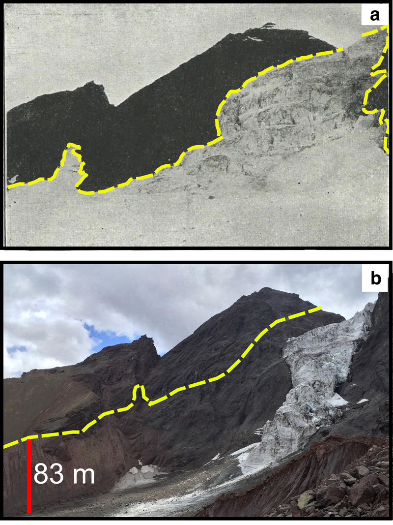
Fig. 5. (a) Photograph taken by Albrecht Maaß in March 1932 of El Morado Glacier. (b) Photograph of the same location taken on 27 February 2018. The dashed yellow corresponds to the interpretation of the ice elevation in 1932.
Figure 6 shows the annual mass-balance estimations for El Morado Glacier between 1980/81 and 2015/16 obtained the minimal surface mass-balance model described in Section 3.7. Overall, a mean cumulative glacier mass balance of −0.71 m w.e. a−1 was observed over the 35-year simulation period, which closely matches the cumulative geodetic mass-balance values obtained from DEM differencing (Table 5). The advantage of the minimal climatic glacier mass balance is that it provides insights into the glacier response to inter-annual climate variability (Fig. 6), which shows overall the predominance of negative mass balance. The hydrological year 1982/83 shows the highest positive mass balance (2.7 m w.e) while the most negative mass balance occurs in the hydrological year 1998/99 (−2.4 m w.e.), which was the driest year in the 1990s. The previous hydrological year (1997/98) shows a positive value of 1.5 m w.e. demonstrating a large inter-annual variability of the glacier mass balance.

Fig. 6. Annual glacier mass balance estimated using temperature and precipitation between 1979 and 2016 as an input.
4.3 Glacier lake evolution
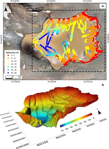
The evolution of the proglacial lake that has developed adjacent to the glacier front is shown in Figure 7. The proglacial lake was first observed in a small form in 1955 (covering an area of 0.01 ± 0.003 km2), meaning it likely began to develop in the early 1950s (Figs 2, 7). Between 1955 and 2019, the evolution of this lake is shown to closely correspond to the changes in the glacier front described above (see Fig. S5), increasing in size by 0.19 ± 0.01 km2 during this period (Fig. 7a). In line with ice front changes, particularly large changes occurred between 2013 and 2019 when the lake area increased by more than 100%. The bathymetric survey results (Fig. 8a) indicate that around the northern, eastern (moraine side), and southern peripheries of the lake water depths ranged between 0 and 15 m. In comparison, maximum depths of 55–68 m (Fig. 8b) were obtained in the central regions of the lake ~85 m from the 2017 calving glacier front. Using these depth measurements, it was estimated that in 2017, the proglacial lake contained 3.6 million m3 of water (±5% uncertainty).
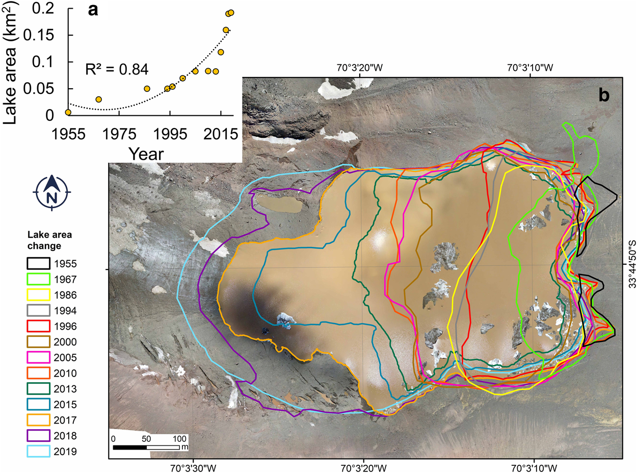
Fig. 7. Growth in the proglacial lake at El Morado Glacier derived from data sources described in the text (a–b). Background image was acquired by a DJI Phantom 4 drone in February 2017.

Fig. 8. (a) Bathymetry survey of the El Morado proglacial lake carried out in 2017. (b) Interpolated 3D model of the bottom of the lake which was used to estimate the lake volume.
In Figure 9, we present the comparison between the glacier surface topographies (DEM 1955–2019) along the centreline illustrated in the longitudinal profile A-A′ (Figs 1, 9), including the frontal positions of the glacier in their respective year, and the bathymetry measurements. Overall, we estimate that the glacier tongue from 1955 to 2000 was grounded and likely until 2009. In Figure S6, we present a set of photographs (summers between 2003 and 2019), where in 2003, we can still observe several metres of thick ice above the lake level, even until 2009. Between these years, we observe several thermo-erosional notches, which are related to temperature lake and several subglacial tunnels in 2009 (Fig. S6). The satellite images and field photographs show no significant changes in frontal position during these years. Between 2005 and 2010, we did not observe changes in the centreline of the glacier, although changes were observed in lateral areas of the glacier tongue with considerable debris cover.

Fig. 9. Longitudinal elevation profile (A-A′) of the centreline (Fig. 1) of the El Morado Glacier tongue between 1955 and 2019, derived from digital elevation models with their respective frontal position and lake bathymetry in 2017.
From 2013 to 2015, the surface of the glacier was relatively flat for ~100 m from the calving front towards the ice cliff. During this period, a depression in the glacier tongue was formed, which is related to the subaqueous process. In this section of the glacier, we obtain the maximum depth in our bathymetry measurements (68 m) and a few metres of flotation thickness, indicating that a large portion of the glacier tongue was floating. This triggered several calving events during the end of 2013 and 2014. We estimate an area loss of 0.03 km2, and ~1 million m3 of water was added to the lake between 2013 and 2015. Between 2018 and 2019, our DEM indicates little difference between the ice freeboard and the waterline, which may indicate that the glacier tongue is slightly floating, assuming as equivalent the last depth values measured (14–26 m depths), which is about 150 m to the front in 2018. During these years, we also observed a large number of icebergs (Fig. 7 and Fig.S6).
5. Discussion
5.1 Glacier changes in the Central Andes of Chile
We have provided a long-term assessment of the response of El Morado Glacier to climatic changes in the 20th and early 21st century. Overall, the data presented reveal a near-continuous trend of glacier retreat and frontal thinning between 1932 and 2019, with ice thinning rates increasing considerably since 2010. The minimal surface mass-balance model presented was able to reproduce the inter-annual variability and shows a similar trend to the geodetic glacier mass balance calculated for the entire glacier between 1955 and 2015 (Fig. 10 and Table 5). The correlation between both methods has been observed for Echaurren Norte Glacier (Masiokas and others, Reference Masiokas2016; Farías-Barahona and others, Reference Farías-Barahona2019). Overall, these observations agree with general climate trends observed elsewhere in the Central Andes of Chile, where increasing ice mass losses and retreat rates have occurred since the middle of the 20th century (Malmros and others, Reference Malmros, Mernild, Wilson, Fensholt and Yde2016; Masiokas and others, Reference Masiokas2016; Wilson and others, Reference Wilson, Mernild, Malmros, Bravo and Carrión2016; Farías-Barahona and others, Reference Farías-Barahona2019). However, in comparison with Farías-Barahona and others (Reference Farías-Barahona2020), which recently calculated a positive glacier mass balance for the Volcan sub-basin between 1955 and 2000, our results present negative values in the almost same study period (1955–1996). These differences are related to the positive glacier mass balance found on the biggest glaciers located at high altitudes by Farías-Barahona and others (Reference Farías-Barahona2000). On the other hand, a wide portion of the glacier tongue is located at low altitude where high thinning rates were observed and likely exacerbated by the proglacial lake, which may negatively influence the total glacier mass-balance estimation.
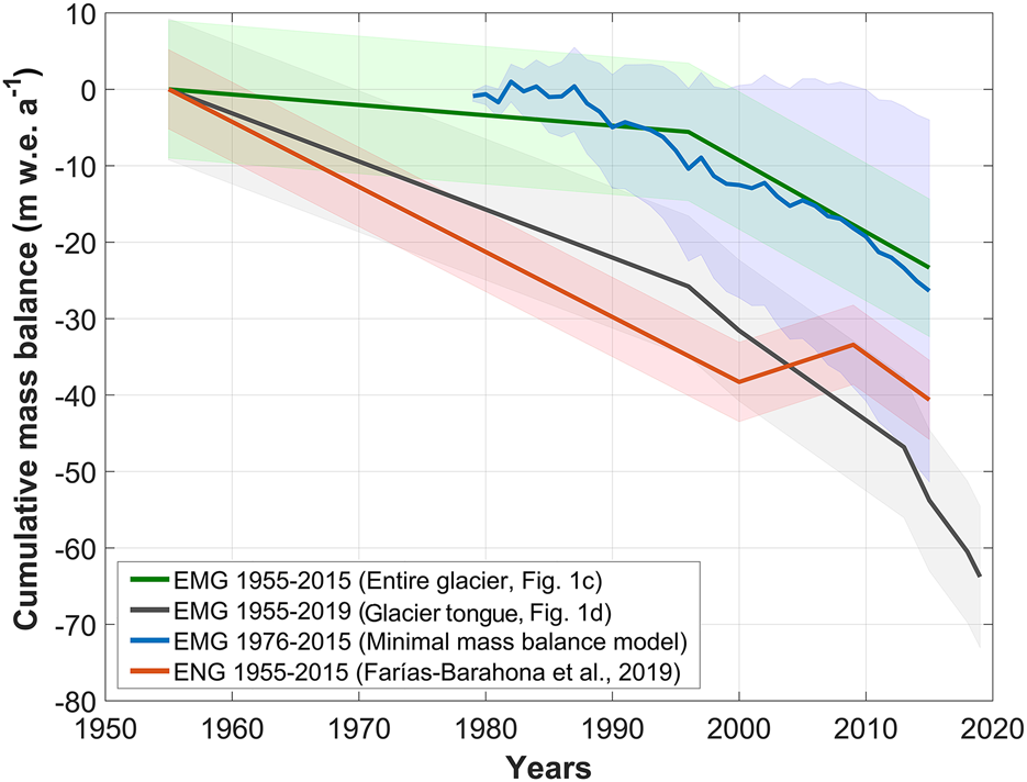
Fig. 10. Comparison of the cumulative geodetic glacier mass balance (entire area and tongue) and climatic mass balance of El Morado Glacier with the geodetic mass balance of the Echaurren Norte Glacier (ENG) (Farías-Barahona and others, Reference Farías-Barahona2019).
The glacier mass balance in the Central Andes of Chile is highly correlated with precipitation (Escobar and others, Reference Escobar, Casassa and Pozo1995, Masiokas and others, Reference Masiokas, Villalba, Luckman, Le Quesne and Aravena2006; Farías-Barahona and others, Reference Farías-Barahona2019). Large interannual variability in precipitation is related to El Niño Southern Oscillation (ENSO). During El Niño (warm) wet phases, increased precipitation is associated with positive glacier mass balance (also neutral), with negative mass balance during cold and dry La Niña phases. However, shifts in precipitation have also been related to other drivers, such as the Pacific Decadal Oscillation (PDO) or the Interdecadal Pacific Oscillation (IPO) (Garreaud and others, Reference Garreaud, Vuille, Compagnucci and Marengo2009; Boisier and others, Reference Boisier, Rondanelli, Garreaud and Muñoz2016; González-Reyes and others, Reference González-Reyes2017).
Due to its proximity and similar elevation to El Morado Glacier, and the availability of long-term direct and indirect mass-balance data, Echaurren Norte Glacier represents an ideal site for comparison with the presented results. Ice elevation changes derived from analyses of topographic maps acquired for Echaurren Norte Glacier reveal considerable cumulative thinning between 1955 and 2000 (−1.00 m a−1) (Farías-Barahona and others, Reference Farías-Barahona2019) similar to that observed here for the glacier tongue between 1955 and 1996. Both direct and geodetic data available for Echaurren Norte Glacier suggest that this period of thinning was followed by a period of positive elevation changes observed between 2000 and 2009 (Fig. 10) (DGA, 2010; Farías-Barahona and others, Reference Farías-Barahona2019). This trend of positive elevation changes has been observed in geodetic mass balance records and through analysis of ice velocity changes available elsewhere in the Central Andes (e.g. Wilson and others, Reference Wilson, Mernild, Malmros, Bravo and Carrión2016; Burger and other, Reference Burger2019; Dussaillant and others, Reference Dussaillant2019). Although our surface elevation changes data do not cover the 2000 to 2009 period specifically, there is evidence in both the frontal change and climatic mass-balance datasets that ice losses during this period were less than usual, with positive mass balances being estimated for both the 2002/03 and 2005/06 hydrological years. Similar patterns of decreased thinning rates were also observed by Burger and others (Reference Burger2019) for Bello Glacier and Yeso Glacier between 2000 and 2013, both of which are located in the Maipo River basin.
Prior to the 2000–2009 period, sustained periods of positive mass-balance behaviour and frontal advance had also been observed for glaciers in the Central Andes during the 1980s, including Echaurren Norte Glacier, Universidad Glacier and glaciers in the Rio Plomo basin, Argentina, among others (Espizua and others, Reference Espizua, Pitte and Ferri Hidalgo2008; Masiokas and others, Reference Masiokas2016; Wilson and others, Reference Wilson, Mernild, Malmros, Bravo and Carrión2016). This trend is also apparent in the climatic mass-balance simulations presented here, and may explain the lower thinning rates observed between 1955 and 1996 (Table 5). Such behaviour may be attributed to the occurrence of a number of warm-phase ENSO events during this period (6 events from 1975) and also several neutral periods with positive mass-balance conditions, through the virtue of increased snowfall supply (Masiokas and others, Reference Masiokas, Villalba, Luckman, Le Quesne and Aravena2006; Farías-Barahona and others, Reference Farías-Barahona2019). A good example of the effect these ENSO events have on levels of snowfall is shown in Figure 2g for the 1982/83 hydrological year. Captured in the summer (January) of 1983, snow cover in Figure 2g is visible below the elevation of the glacier tongue and beneath the local Equilibrium Line Altitude (ELA) (Carrasco and others, Reference Carrasco, Casassa and Quintana2005). Interestingly, this hydrological year corresponds with the highest positive mass-balance values recorded for Echaurren Norte Glacier (Masiokas and others, Reference Masiokas2016; WGMS, Reference Zemp, Nussbaumer, GärtnerRoer, Huber, Machguth, Paul and Hoelzle2017; Farías-Barahona and others, Reference Farías-Barahona2019) and simulated here (Fig. 6).
The increasingly negative mass-balance trend observed since 2010 has been similarly observed in the glacier records available for the Maipo River basin (Farías-Barahona and others, Reference Farías-Barahona2020), Echaurren Norte Glacier (Masiokas and others, Reference Masiokas2016; Farías-Barahona and others, Reference Farías-Barahona2019) and presented by Wilson and others (Reference Wilson, Mernild, Malmros, Bravo and Carrión2016) (Universidad Glacier) and Burger and others (Reference Burger2019) (Bello, Yeso and Piramide Glacier). The acceleration in glacier losses observed in the Central Andes in general has been linked to the so-called mega-drought, a prolonged and unprecedented dry period experienced across this region since 2010 (Garreaud and others, Reference Garreaud2017, Reference Garreaud2019).
Although the glacier contribution to runoff at basin scales in the Central Andes is minor compared to other components (snow, rainfall) (Masiokas and others, Reference Masiokas, Villalba, Luckman, Le Quesne and Aravena2006; Ayala and others, Reference Ayala2020), previous hydrological studies have highlighted the importance of glacier contributions in the Maipo River basin during dry periods. During the severe drought of 1969, one of the driest summers on the hydro-meteorological record, about 67% of the total runoff at the outlet of the basin was originated from glacier meltwater (Peña and Nazarala, Reference Peña and Nazarala1987). This high dependence on glacier meltwater during dry periods has been re-confirmed more recently by other authors (i.e. Casassa and others, Reference Casassa2015; Ayala and others, Reference Ayala2016, Reference Ayala2020). The 2010-present drought has been described as unprecedented in the historical record, due to its duration and spatial extent (Garreaud and others, Reference Garreaud2017, Reference Garreaud2019). There are several lines of evidence indicating that the surface hydrology, groundwater and vegetation has been affected as a consequence of this severe drought (Garreaud and others, Reference Garreaud2017) including an acceleration in glacier thinning rates (Burger and others, Reference Burger2019; Dussaillant and others, Reference Dussaillant2019; Farías-Barahona and others, Reference Farías-Barahona2019, Reference Farías-Barahona2020). It is noteworthy that several neutral phases of El Niño have occurred during this drought period (Garreaud and others, Reference Garreaud2017) that can sometimes correspond to periods of positive glacier mass balance. In this case, however, such glacier behaviour has not been observed (Escobar and others, Reference Escobar, Casassa and Pozo1995; Farías-Barahora and others, Reference Farías-Barahona2019).
Besides the precipitation deficit, previous studies indicated a temperature increase for the Central Andes of Chile (Falvey and Garreaud, Reference Falvey and Garreaud2009), with a noticeable increase in the autumn and spring temperatures of inland Maipo (Burger and other, Reference Burger, Brock and Montecinos2018). Moreover, from 2016 to 2019, a sequence of peaks in the absolute temperature were observed, including the highest temperature recorded in Santiago city during January 2019 (DMC stations). This may also explain the highest thinning rates found between January and March of 2019 (−2.68 ± 0.20 m a−1) in the glacier tongue, but also the high glacier area reduction observed between 2015 and 2019. If the current drought persists, it is likely that the recent period of accelerated ice losses observed in the Central Andes will continue. Such a scenario highlights the need for continual monitoring of glaciers in this region in order to better understand downstream impacts. Overall, the similarities in the geodetic and climatic mass-balance trends presented here and by others for glaciers elsewhere in the Central Andes suggest that the methods described offer a reliable approach for investigating glacier change in the Central Andes and in other glacierised environments where field measurements may not exist.
Compared to glacier mass-balance analyses, glacier area and front changes have been studied in far more detail across the Central Andes of Chile (e.g. Rivera and others, Reference Rivera, Acuña and Lange2000; Malmros and others, Reference Malmros, Mernild, Wilson, Fensholt and Yde2016; Farías-Barahona and others, Reference Farías-Barahona2019). These studies have highlighted considerable ice area losses since 1955. For instance, glaciers in the Olivares sub-basin (Maipo River), the largest in the Central Andes, have been shown to have retreated in area by an average of 30% between 1955 and 2013 (Malmros and others, Reference Malmros, Mernild, Wilson, Fensholt and Yde2016). These retreat rates are similar to our findings for El Morado Glacier, which has also shown to have reduced in area by 40% between 1955 and 2019. In comparison, the Echaurren Norte Glacier has reduced in area by 65% over a 60-year period (Farías-Barahona and others, Reference Farías-Barahona2019). This difference in areal reduction is likely the result of differing hypsometry and aspect.
5.2 Glacial lakes and glacial lake outburst flood hazard
The thinning and retreat of El Morado Glacier has resulted in the development and considerable expansion of an adjacent proglacial lake in recent years. In the Central Andes, proglacial lakes are normally developed in over-deepened basins vacated by receding glaciers and dammed by moraines and ice, although temporary glacial lakes also exist formed by episodic glacier advances (Iribarren and others, Reference Iribarren Anacona, Mackintosh and Norton2015). Wilson and others (Reference Wilson2018) recently identified the existence of a total of 313 glacial lakes in the Central Andes in their 2016 inventory of the region. However, up until now, none of these lakes have been surveyed in detail in regards to their bathymetry, limiting our ability to quantify their significance as water stores. Hence, the results presented for the proglacial lake provide new insight about the current status of this specific glacial lake system and detail the impacts of recent glacier change. Considering the ice losses presented for El Morado Glacier, it is unsurprising that its proglacial lake has grown in area dramatically since its emergence in the early 1950s. This behaviour is in line with glacial lake trends that have been observed across the Chilean Andes (Wilson and others, Reference Wilson2018) and other glacierised regions elsewhere (Wang and others, Reference Wang, Xiang, Gao, Lu and Yao2015; Emmer and others, Reference Emmer, Klimes, Mergili, Vilimek and Cochachin2016; Watson and others, Reference Watson2020). The importance of glacial lakes is threefold: (1) they represent a considerable water resource by storing meltwater (Haeberli and others, Reference Haeberli2016); (2) they can exacerbate the glacier mass loss (e.g. King and others, Reference King, Bhattacharya, Bhambri and Bolch2019); and (3) in some instances they represent considerable glacial hazards, having in the past been the source of a number of high-magnitude glacial lake outburst floods (GLOFs) (e.g. Wilson and others, Reference Wilson2019). Generated by the failure of ice- and moraine-dammed lakes, GLOFs have the ability to travel large distances downstream and can pose a significant threat to downstream infrastructure, agricultural land and human settlements (Kääb and others, Reference Kääb, Reynolds, Haeberli, Huber, Bugmann and Reasoner2005; Keiler and others, Reference Keiler, Knight and Harrison2010; Carrivick and Tweed, Reference Carrivick and Tweed2016). In the Central and Patagonian Andes, >30 GLOF events have been identified since the 1980s as a result of ice/moraine dam failure (Iribarren Anacona and others, Reference Iribarren Anacona, Mackintosh and Norton2015; Wilson and others, Reference Wilson2018). The majority of the GLOF events have occurred in Patagonia, where the climate, glaciological and topographical setting has promoted the growth of lakes behind lateral/terminal moraines, ice dams and within de-glaciated valley bottoms. However, GLOFs have also been observed in the Central Andes, most notably at Cachapoal Glacier in 1981 (Peña and Klohn, Reference Peña and Klohn1990) and Juncal Sur Glacier in 1954 (Peña and Klohn, Reference Peña and Klohn1990). In other Andean countries, such as Peru, GLOFs have been directly responsible for thousands of deaths (Reynolds, Reference Reynolds, McCall, Laming and Scott1992; Carrivick and Tweed, Reference Carrivick and Tweed2016; Mergili and others, Reference Mergili2020).
In conjunction with the surface topographies (DEMs 1955–2019), our bathymetric survey provides new insight about the evolution of the proglacial lake. Overall, different processes and mechanisms can be observed through time. The development and increase in the size of the lake appear to be linked to subaerial glacier elevation changes, subaqueous processes such as calving and ice-cliff collapse. Glacier calving depends on factors including water temperature, debris cover, glacier velocity and bed topography (Rohl, Reference Rohl2006; Benn and others, Reference Benn, Warren and Mottram2007; Watson and others, Reference Watson2020). Our observations between 2000 and 2010 suggests that calving above the waterline was driven by a thermal-erosional notch (Rohl, Reference Rohl2006). This seasonal effect related to the water temperature is observed in the field photographs during the summers of 2003, 2009 and 2019 (Fig. S6). Once the notch is formed, increments in the stress of the closest crevasse tip result in ice cliffs that become detached from the glacier front, generating icebergs. After 2010, the increase in lake area is coincident with the drought period, and a considerable increase in the water volume occurred, especially between the years 2013 and 2015 when a large portion of the glacier tongue was floating and 1 million m3 of water was added to the lake. During the summer of 2014, we observe temperatures up to 9 °C at 3400 m a.s.l (Fig. S3), which likely accelerated the calving process. From 2015 onwards, the glacier lake area increased exponentially (Fig. 7), and this may be linked with the sequence of high temperatures recorded until 2019.
The bathymetric survey presented for the proglacial lake is the first of its kind in the Central Andes, which restricts comparisons across sites. However, our results can be compared with empirical relationships that use area, depth and volume scaling (e.g. Huggel and others, Reference Huggel, Kaab, Haeberli, Teysseire and Paul2002; Cook and Quincey, Reference Cook and Quincey2015). Scaling approaches allow glacial lake volumes to be estimated in data-poor regions. For the Central Andes, Wilson and others (Reference Wilson2018), for example, estimated a total volume of 0.34 km3 for moraine-dammed lakes in 2016 using the volume-area scaling. Cook and Quincey (Reference Cook and Quincey2015) compared several empirical scaling relationships in different geomorphometric context. Using a compilation of 42 glacial lake datapoints (including duplicate sites), they derived a depth (D)–area (A) relationship of D = 0.5057A 0.2884. Applying this relationship to the proglacial lake, we observed an underestimation of total water volume by ~30% in comparison to our direct measurements (±5%). A similar underestimation is also evident when applying the depth–area relationship of D = 0.104A 0.42 suggested by Huggel and others (Reference Huggel, Kaab, Haeberli, Teysseire and Paul2002). The existence of such discrepancies between empirically- and directly-derived lake volumes likely results from the existence of complex lake geometries (Cook and Quincey, Reference Cook and Quincey2015). Nevertheless, what these differences highlight is the importance of acquiring direct measurements of glacial lake depth, particularly in the context of assessing GLOF hazard, which requires a good understanding of a lake's total and effective water volume (Richardson and Reynolds, Reference Richardson and Reynolds2000; Wilson and others, Reference Wilson2019).
In terms of GLOF hazard, in its current state (as of 2019), the proglacial lake level is 3–6 m below the crest of its impounding moraine, meaning that overtopping through increased water input, depends largely on the remaining water volume available in the glacier tongue. Alternatively, a future GLOF event could occur from a failure in the dam moraine or as the glacier continues to retreat, there may be a hazard of dam overtopping through the generation of waves, resulting from ice falls sourced from the glaciers steep overhanging ice cliff. This assumption depends very much on the scale of future glacier/lake changes and therefore further monitoring and detailed assessment of the basin is recommended given its close proximity to human settlements (e.g. Baños Morales village) and hydropower infrastructure (Fig. S7). The occurrence of GLOF events across the Andes has highlighted the need for regional-scale assessments of GLOF/glacial lake distribution (such as those presented by Wilson and others, Reference Wilson2018) coupled with detailed topographic and bathymetric surveys of specific lakes of interest (such as that presented here). These analyses should help inform glacial hazard assessments and climate change mitigation efforts in glacierised regions.
6. Conclusions
This study presents a detailed and long-term assessment of the response of El Morado Glacier and its adjacent proglacial lake. The assessment focuses on four indicators of glacier behaviour: (1) changes in ice surface elevation (1932–1955–2019); (2) changes in glacier area and frontal positions (1955–2019); (3) proglacial lake area change (1955–2019); and (4) changes in climatic mass balance (1979/80–2015/16). These analyses were achieved through the use of multi-temporal aerial/terrestrial photography, satellite imagery and LiDAR data, and the so-called minimal mass-balance model combined with direct and indirect climate data. We obtain a mean geodetic glacier mass balance of −0.39 ± 0.15 m w.e. a−1 for the entire area between 1955 and 2015 and area change of 0.61 km2 (40%) between 1955 and 2019. For the glacier tongue specifically, a total mean elevation change of −1.18 ± 0.22 m a−1 was observed between 1955 and 2019, with a distinct increase of ice thinning rates and area changes observed during the recent decade. Considering the ice surface information obtained from the 1932 terrestrial photography, we obtain an ice-elevation change rate for the glacier tongue of −1.00 ± 0.17 m a−1 until 2019 (87 years). Results of our minimal surface mass balance are in line with the glacier mass balance observations derived from DEMs, which also shows the prevalence of negative values during the recent severe drought. In terms of the evolution of the proglacial lake, results reveal that the lake likely first developed in the early 1950s having obtained an area of 0.01 km2 by 1955. In contrast to the glacier tongue, the lake continued to grow over the following 64 years and covered an area of 0.19 km2 in 2019. Lake bathymetry data collected in 2017 reveal a maximum water depth of 68 m. Using these data, a total water storage of 3.6 million m3 (±5%) was calculated.
Overall, the data presented reveal a general trend of retreat and frontal thinning at El Morado Glacier since 1932, with an acceleration of these ice losses occurring since 2010. Through comparison with data available for other glaciers in the Central Andes, this study highlights that such behaviour is not isolated to El Morado Glacier, and may indicate a wider regional trend. The most direct impact of these glacier losses on a basin-scale is the change in the availability of meltwater. A combination of factors such as the reduction in precipitation amounts and snow cover, and the occurrence of an extreme drought event, has put increased pressure on glaciers as a water resource in the Central Andes.
Supplementary material
The supplementary material for this article can be found at https://doi.org/10.1017/jog.2020.52.
Acknowledgements
We greatly acknowledge the Aero-photogrammetric Service (SAF) and the Geographical Military Institute (IGM) for the aerial photographs. Meteorological and LiDAR data were kindly provided by DGA, TLS data from 2015 by Geocom S.A., TanDEM-X data by DLR under project AO XTI_GLAC0264 and Landsat TM by USGS. CR2MET gridded climatology (http://www.cr2.cl/datos-productos-grillados/) was provided by CR2. We acknowledge Mark Neal (Ystumtec Ltd.) for designing and building the bathymetry boat used in this study, and the Deutscher Andenverein (DAV) – Club Andino Alemán, Chile for the mountaineering report (in http://www.dav.cl). D.F-B, C.B and A.C acknowledge the support of ANID through the doctoral scholarships program. D.F-B thanks the Fränkischen Geographischen Gesellschaft for funding a field campaign and F413. This work was conducted as part of the ‘Glacial hazards in Chile: processes, assessment, mitigation and risk management’ project which is jointly funded by the UK Natural Environment Research Council (NERC) (grant NE/N020693/1) and the Chilean Natural Commission for Scientific and Technological Research (CONICYT) (grant MR/N026462/1). Additional support was given by the Chilean National Science Foundation (Fondecyt) under grant agreement no. 1161130. The Friedrich-Alexander-Universität Erlangen-Nürnberg provided funding within their program Open Access Publishing Fund. Finally, we thank the editor Dan H. Shugar and the reviews from Simon Cook and Umesh Haritashya, whose suggestions and comments helped to significantly improve the manuscript. We also give thanks for the final remarks given by chief editor Hester Jiskoot.
Author contributions
D.F-B design the study, measured LiDAR TLS, GNSS, processed InSAR, all the optical datasets, elevation changes and wrote the manuscript. R.W., O.W. and S.H measured and processed the bathymetry data and drone aerial photographs. S.V and D.F-B process and post-processed the DEMs with SfM, A.C, G.C, and D.F-B., measured the LiDAR TLS and GNSS. T.S., and A.M., measured the TLS in 2019. C.B. calculated the SMB. A.A, J.Mc, N.F.G, provided feedback throughout the study. M.H.B. lead the study. All the authors revised the manuscript.


 Open access