


Abstract
A simple experiment based on thermal imaging is devised to observe and measure, along a cooling fin in contact with a hot spot, the temperature profile determined by conductive and convective heat transport. By using a simple theoretical approach, the cooling fin equation is justified and applied to describe, in an educational framework and perspective, the experimental results. Both the experimental setup and the theoretical model discussed in this work are suited for undergraduate physics students.
Export citation and abstract BibTeX RIS
1. Introduction
Infrared thermal imaging is an increasingly convincing and effective way to discover, observe, discuss and interpret heat transport phenomena at basically every educational level, even in an informal framework [1–4]. The adoption of this technique has been a more widespread approach since the introduction of relatively inexpensive smartphone adapters which make the infrared detection and measurement quite affordable [5]. Typical applications are in the field of the analysis of temperature distribution and the associated changes in solid and liquid bodies mostly when remote sensing is needed. The discussion about thermal energy transport, as it is well-known, is addressed in many chapters of both fundamental and applied classical physics, with special attention to the distinction among conduction/convection and radiative mechanisms [6]. The majority of thermal imaging studies in an educational perspective are associated with stationary configurations. Much less has been done about transient temperature fields also in view of their greater difficulty from a theoretical and mathematical viewpoint. Moreover, convective mechanisms are only considered at a very technical, engineering-like level [7–10]. As such, they are barely addressed in the basic treatments of introductory thermodynamics courses and textbooks. Because of the semi-empirical nature of the governing laws for convection mechanisms, educational approaches do not devote much attention to possible applications of these kinds of problems. Convection processes are nonetheless a crucial aspect in every practical situation where temperature gradients are relevant and fluid transport phenomena play a determinant role. The typical approach to convective mechanism in education research refers to the Newton cooling law [11, 12]. According to it, through a time analysis of the exponential decrease of temperature of a warm object in a colder fluid, it is possible to determine the characteristic time constant which, in turn, contains information on both the body thermal capacity and on the convective parameter of the fluid.
In this work, which continues and extends a previous research [2], the focus is on the deduction of a simplified, time-independent heat equation when both conduction and convection are present. The associated experiment being proposed here is a basic setup which resembles the functioning of typical cooling systems, such as the fin at the basis of the heat sinks for electronic components. A simple, standard configuration (a single cooling plate) is visualized in its operational aspects thanks to a continuous thermal monitoring based on infrared imaging. As an appealing feature, this approach allows for a direct, even if approximated, estimate of the convective parameters of the fin configuration in use which, in turn, can be used to understand on a semi-quantitative basis the concept and substance of thermal resistance. Some aspects about the dependence of the convection parameter on the fluid speed are also addressed.
All the following considerations and measurements need an appropriate understanding of the advantages as well as the weak points which characterize the operation of an infrared thermal camera, as discussed elsewhere [1, 2, 13]. Here, we limit to emphasize that temperature is a 'side-product' of the detecting process, since the sensor just acquires electromagnetic radiation approximately in the 8–14 μm range which is converted to temperature values according to a black-body behavior and with an emissivity calibration which can be very critical: IR cameras are not thermometers. Yet, keeping in evidence the qualitative, demonstrative and educational purposes of this approach, a very suggestive and practical visualization and interpretation of temperature profiles and fields can be obtained.
2. Thermal energy transfer: the fin equation
We are interested here in the model describing heat flowing from a body at relatively high temperature to a colder external environment. The simplest approach makes use of the Newton's cooling law, whose most relevant features can be found in various textbooks, such as in references [6, 7]. Here, one needs to recall that the heat transfer rate  (measured in watt: one can also work with the heat flux, i.e. the heat transfer rate per unit area, measured in W m−2) can be expressed, for a solid object at temperature TB with a surface S exposed to the environment—the external fluid—at temperature T0, in terms of the convective constant h (measured in W K−1 m−2) as

As illustrated schematically in figure 1, besides the heat transfer rate of equation (1), one can also address the situation in which energy is carried to the external environment by means of a surface extension realized with a solid plate in contact with the hot body. This extension—the cooling fin—because of heat conduction within itself, will expose to the convective flux a larger area thus improving energy dissipation from the hot spot. The plate contribution can be included in the cooling law after some simple assumptions also in view of the experiment here discussed and, more importantly, in order to maintain the mathematical treatment at a very basic level. First, we consider a rectangular plate with constant rectangular section Sbase = Hδ as depicted in figure 1. We then write the energy balance for a thin element with length Δx. If one accounts for both conductive and convective contributions the balance equation is

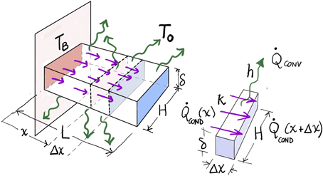
Figure 1. Convective and conductive contributions (constants h and k) to the heat transfer in a thin rectangular plate.
Download figure:
Standard image High-resolution imageFor this same element the convective rate is given by

in which the lateral surface of the plate is Sfin = (2ΔxH) since both its sides (with width H) are exposed to the environment. We assume that the plate is a very thin one, i.e. its edges do not contribute to the diffusion of heat dissipation by convection. The conductive terms obey the usual Fourier law for heat transport through a thin slab of depth Δx and thermal conductivity k (whose units are W K−1 m−1):

Here, the involved surface is the base of the plate, Sbase = Hδ, since the conductive mechanism is supposed to occur in the slab longitudinal direction, i.e. perpendicular to the base section of the plate. We can now combine equations (2)–(4) to obtain, after a simple algebraic manipulation:

We recognize on the left side of this expression the finite-difference, forward approximation to the second-derivative of temperature in the x direction. This means that, in the continuous limit, equation (5) becomes an ordinary differential equation of the constant-coefficient type:

in which we introduce the parameter

whose units are reciprocal length, m−1. Equation (6) is the driving differential equation for the combined conduction–convection mechanism along the rectangular thin fin with thermal conductivity k and immersed in the fluid medium with convection constant h. Note that equation (6) depends only on the slab thickness δ but not on its length L nor its width H. Its general solution is

The particular solution is obtained in terms of the boundary conditions. These are simply defined: first, at the left side (hot surface at x = 0) the temperature is TB. At the opposite side of the fin, x = L, there can be various situations. In this work we assume that at the end of the plate no heat will be transported because of the negligibly small surface of the fin's base. In other words, the temperature gradient at x = L must be zero. Overall, the boundary conditions are

The particular solution compatible with equation (9) is readily obtained and can be expressed, after transforming real exponentials in the hyperbolic cosine for matters of a more compact notation, as

It is possible to achieve also an analytical expression for the heat transfer rate at the fin base and going through the plate (i.e. the total energy transferred per unit area due to both conduction and convection) according to the Fourier law which, after a straightforward manipulation starting from equation (10), leads to

This same result can also be recovered after integration along the fin surface of the convective heat flux (which is responsible of the thermal energy 'removal' from the plate whose temperature distribution is established according to the conductive mechanism):

The final result is in agreement with equation (11) and it allows a direct calculation of the dissipated power at the hot spot.
Before testing this model with some measurements, it is worth recalling two technical definitions speaking of heat sinks, namely the fin efficiency, η, and its efficacy, ε [6, 8]. The main idea is that, because of the presence of an extended surface such as that offered by the fin, the convection processes will amplify the heat removal from the hot point. This happens because of the temperature difference between the hot surface and the colder, external medium; the effect is maximized with relatively high temperature gradients. This will occur at its best when the surface of the fin has the highest possible temperature. Yet, because of heat conduction through the plate, its temperature drops from the hot point value TB to smaller and smaller values. This effect has greater relevance for poor thermal conductors, in which the temperature falls more rapidly along the fin toward the external fluid temperature T0. One can then define the efficiency η of the fin by just comparing the largest heat flux obtainable with a perfect conductor (infinite conductivity, with a constant temperature distribution TB along its full extension) and the real flux above computed and given by equation (11):

We are also interested in the so called efficacy ε of the fin which is obtained by comparing the heat transferred by a convective mechanism at a given hot surface with and without the fin itself (the latter being obtained by simply considering the convection through the base of the fin). The efficacy is then defined as

We notice that efficiency and efficacy are strictly related since one can write

In any case, the efficiency is always smaller than unity. The fin is considered as efficacious only when ε > 1 (otherwise the fin would be an obstacle rather than an advantage to the heat removal). See also figure 2.

Figure 2. Schematic representation of fin efficacy (associated with conductive temperature drop) and efficiency (associated with the fin surface); see text.
Download figure:
Standard image High-resolution imageAnother parameter which is often used in the thermal energy balance and cooling processes is the thermal resistance R of the fin [6], defined according to

With this definition, the units of R are kelvin/watt (K W−1). Another way to measure this property is by means of the heat flux which leads to the thermal specific resistivity, measured in m2K W−1, according to the European ISO regulation 6946 [6, 14]. For the thin rectangular plate with basis Sbase and lateral surface Sfin, according to the equations defining the efficiency/efficacy, the resistance R can also be written as

This to say that, for a given convective constant h, the thermal resistance decreases for more effective and efficacious fins. A smaller resistance implies that a higher power can be transmitted to the environment for a given temperature step TB − T0 (which is usually fixed by operative constraints). The knowledge of these parameters is thus of central relevance for the correct understanding and a proper design of cooling setups such as heat sinks in electronic devices and other thermal apparatuses.
It is with these premises that we now address some simple, practical measurements with the infrared imaging technique.
3. Experimental method and results
The cooling effect produced by conduction/convection can be observed by taking temperature measurements of a metallic plate in thermal contact with a hot source, such as a powered electronic device. In this work, we adopt a simple setup in which the hot device is an electric resistance (10 Ω, 10 W) powered by a DC supply (constant current 1 A). Plates of various lengths (made of brass Cu70/Zn30 in this experiment, with thermal conductivity kbrass = 111 W K−1 m−1 [15]) can be joined to the resistor as shown in figure 3 and in figure 4. The plate here plays the role of the cooling fin and its surface is photographed with the smartphone infrared camera (FlirOne Pro: its main features are the thermal pixel size, 12 μm, thermal resolution of 160 × 120 pixel, thermal sensitivity of 0.07 K, temperature range of −20 to 400 °C, spectral range 8–14 μm, IFOV about 3 mrad/pixel [5]). Fins were painted with matte black silicone spray paint since its emissivity (0.95) can be set to this same value in the IR camera configuration. Temperature values are obtained via the analysis software FLIR Tools (freely distributed by the IR camera manufacturer [16]) which allows to capture temperature profiles in any portion of the IR picture after conversion of the graphical/thermal FLIR public format (FPF); see figure 5. Measurements were done in various convective conditions. More specifically, we considered a natural convection mechanism (the experiment was performed in still air) as well as a forced ventilation configuration (the fin was exposed to moving air produced by a fan at various distances/air speeds). This was done with the aim of obtaining information about the convection parameter as a qualitative function of the environmental arrangement. All these measures have been carried out with reasonable accuracy and attention to the relevant parameters. Yet, and as already pointed out above, given the introductory, educational and illustrative purpose of this work, as well as in view of the features of a temperature acquisition with a non-professional IR camera, the results reported in the following are not to be adopted as a technical, quantitative reference for engineering studies and quantitative projects.
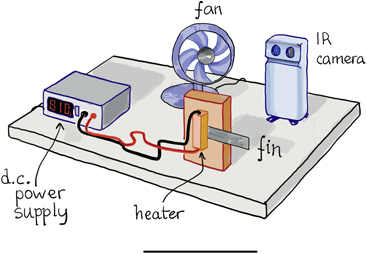
Figure 3. Artist's view of the apparatus.
Download figure:
Standard image High-resolution image
Figure 4. The experimental setup: the FLIR One IR camera is plugged in the right side of the smartphone.
Download figure:
Standard image High-resolution image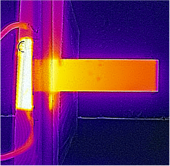
Figure 5. A typical IR picture of the heated fin. Numerical values of temperatures are obtained via a software (FLIR Tools) compatible with the thermal FLIR public format (FPF) of this kind of images.
Download figure:
Standard image High-resolution imageWe have first considered the temperature behavior along the fin and compared their thermal profiles with the model of equation (10). The comparison has been done by fitting, leaving as adjustable parameters the hot spot temperature TB and the coefficient μ for various fin lengths and convection configuration (still or moving air). It is possible to compare the fitted TB temperature with the temperature of the heater in contact with the fin (temperatures can be of course measured with standard thermocouple sensors: this allows also a rough calibration of the temperature determined via the infrared reading which is, as already mentioned, subject to the typically unknown emissivity of the body under exam). The parameter μ is instead used to obtain an estimate of the convective constant h according to equation (7). Determining the convective constant is by no means a trivial task (it is usually an extremely complex function of geometric, thermal, fluid statics and dynamical features of the configuration under exam [17]) but in this experiment one can obtain a workable and direct guess of its value.
We show in figure 6 three series of three plots each: the series are temperatures values along three different brass fins of lengths L = 45, 65 and 85 mm (values within ±0.5 mm), thickness δ =  mm, width H =
  mm. In each series, the three plots refer to the three above mentioned different convective configurations. These are named as L, M and H, which stand for low, medium and high ventilation, respectively. The 'low' setting is the natural convective configuration (i.e. still air is the only responsible for external heat exchange). Medium and high configurations are obtained forcing the ventilation at two different speeds (a hairdryer was set at two fan levels with the air heater switched off). In the plots of figure 6 the dots are temperatures acquired, as already said, with the analysis software of the FLIR camera. Temperature uncertainties are, according to factory specifications, ±5% or ±3 °C (the worse of the two). Geometrical uncertainties, associated with positions along the fin, are smaller than those of the IR camera which are in the 2–3 mm range given the IFOV at a distance of about 25 cm. There are several comments that can be done looking at figure 6. First, we like to point out the overall quality of the fitting procedures. The correlation coefficient is always larger than 0.99 with a least-squares optimization (bases on a proprietary fitting app included in the Matlab® platform [18]) over the temperature curve predicted by equation (10). This fact implies that the convection/conduction model here adopted is an acceptable ansatz for the observed temperatures: their values decrease for increasing distances from the hot spot, as expected because of the conduction through the fin body. It is also interesting and noticeable here to observe the differences for the convective actions (the L, M, H cases), i.e. the temperature reduction caused by still/moving air which is indeed the main reason for adopting the heat sink system. This aspect can be described after determination of the convective constant h. As above pointed out, h is obtainable directly according to its inclusion in equation (7), where the parameter μ is directly fitted on the temperature curve, equation (10). We report in table 1 values of h for the 9 series of figure 6. Here and in the following, uncertainties on the fitted parameter μ have been determined from the associated 95% confidence bonds whilst uncertainties for other quantities are obtained via standard direct error propagation on their defining relations. We observe that in the still air regime ('L') the convective constant is about 13 W K−1 m−2, independently from the fin length. This suggests that the fitted value of h can be adopted as a reasonable estimate of the 'true' convective constant for this configuration (i.e. what is expected in absence of forced ventilation mechanisms which instead could depend more strictly on the geometry and spatial orientation of the cooling element and, of course, on air speed). We notice in fact that h changes differently for the three plates in presence of moving air. In particular, we obtain a regular increase of h with increasing air speed but a slight decrease with longer fins. This last fact could be interpreted by accounting for the uneven distribution of the air flow on the fin surfaces, becoming more evident for longer plates. Moreover, the value of h in still air is in fair agreement with the literature reference, even if values up to about 50 W K−1 m−2 are expected for moving air at room temperature [19, 20] as is in fact obtained in our experiment.
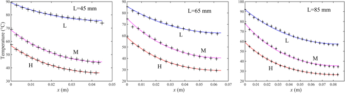
Figure 6. Temperature fields (dots) and fitting models (continuous curves) for three brass plates of different length in three convective configurations (low, medium, high), see text. The x-axis is the distance from the hot spot at temperature TB. Air room temperature was T0 = 19.5 ± 0.5 °C.
Download figure:
Standard image High-resolution imageTable 1. Fitted values of the parameter μ (m−1) and the associated convective constant h (W K−1 m−2) obtained from equation (7) for the three plates in the three (low, medium, high) cooling regimes. Uncertainties for the fitted parameter μ are the 95% confidence bounds of the fitting procedure whilst those of h are propagated from those of μ and δ, once again from equation (7).
| Low | Medium | High | ||||
|---|---|---|---|---|---|---|
| L (mm) | μ | h | μ | h | μ | h |
| 45 | 15.0 ± 0.2 | 13 ± 3 | 28.5 ± 0.1 | 45 ± 9 | 31.6 ± 0.1 | 55 ± 11 |
| 65 | 15.3 ± 0.1 | 13 ± 3 | 24.9 ± 0.1 | 34 ± 7 | 31.0 ± 0.1 | 53 ± 11 |
| 85 | 14.8 ± 0.1 | 12 ± 2 | 23.0 ± 0.1 | 29 ± 6 | 28.0 ± 0.1 | 44 ± 9 |
Thermal efficiency/efficacy/resistance of the fins in various cooling configurations can also be determined by simply applying equations (13)–(17) to the fitted/computed values of μ and h. Results are reported in table 2. As a general comment, we observe that the efficiency η decreases with increasing fin's length since this implies a larger temperature drop along the fin itself and, as a consequence, a lower convective action. This is true for all three cooling strengths. The efficacy ε instead increases with the length L because of the larger exposed surface in comparison with the naked hot element. We also observe that efficacy/efficiency for a given fin length decreases with increasing ventilation. This rather counter-intuitive effect is explained since the heat flux of the fin, expressed by equation (11), for a large convective parameter h behaves as  whilst the maximum heat flux (without any conductive temperature drop) is in the form hΔT. On consequence, the efficiency behaves as h−1/2, i.e. it decreases with increasing h. The same happens for the efficacy since, for a given length L, ε /η = const.
Table 2. Fitted values of efficacy ε, efficiency η and thermal resistance R (kelvin/watt) of the brass fins in the three convection configurations. Absolute uncertainties obtained via error propagation of the computed 95% confidence interval for the fitted parameter μ.
| L (mm) | 45 | 65 | 85 | ||||||
|---|---|---|---|---|---|---|---|---|---|
| Ventilation | ε | η | R | ε | η | R | ε | η | R |
| Low | 78 ± 7 | 0.87 ± 0.01 | 43 ± 5 | 99 ± 8 | 0.76 ± 0.01 | 32 ± 4 | 115 ± 9 | 0.68 ± 0.01 | 30 ± 3 |
| Medium | 60 ± 5 | 0.67 ± 0.02 | 15 ± 2 | 74 ± 6 | 0.57 ± 0.01 | 16 ± 2 | 84 ± 6 | 0.49 ± 0.01 | 17 ± 2 |
| High | 56 ± 5 | 0.63 ± 0.02 | 13 ± 2 | 62 ± 5 | 0.48 ± 0.01 | 13 ± 1 | 70 ± 5 | 0.41 ± 0.01 | 14 ± 2 |
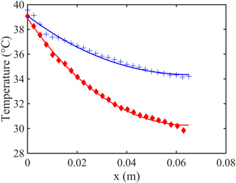
It is also possible to account for the direct effect of thermal conductivity by employing fins made of different materials. We show as an example in figure 7 temperatures profiles and the corresponding fitting curves of two fins with equal shapes/sizes made by brass and aluminum (here a die casting alloy, whose thermal conductivity is 205 W K−1 m−2 [15]). The steeper temperature drop of the less conducting plate (i.e. the brass one) is evident. We are interested here in the efficiency/efficacy of the plates which result both larger for the more conductive fin (i.e. the aluminum one). More explicitly, for the configurations shown in figure 7, one obtains ηAl = 109 ± 9, ηbrass = 92 ± 7 and ɛAl = 0.84 ± 0.01, ɛbrass = 0.70 ± 0.01. This is one of the reasons why aluminum is appropriate for cooling devices (besides its cost and light weight): it leads to a higher heat flux and energy dissipation for a given temperature jump.
Figure 7. Observed temperature profiles and fitting model for two fins: aluminum (blue crosses) and brass (red diamonds). The x axis is the distance from the hot spot. Both fins were in the 'High' ventilation configuration. Length L = 65 mm. Fitted hot spot temperature: TB = 40 °C.
Download figure:
Standard image High-resolution image
4. Conclusions
With a simple experimental setup including a smartphone-based infrared camera for thermal imaging, we show some significant features of a conduction/convection cooling system. The heat transfer equation in presence of stationary convective effects has been obtained in its simplest form and implemented as a fitting model to the observed temperature fields which in turn have been acquired via infrared imaging. The fitted parameters can be used to achieve a fair approximation to the convective constant of still or moving air in the simple rectangular geometry here adopted for the heat sink. Besides, thermal efficiency, efficacy and resistance of the cooling system are also estimated and briefly commented to show the validity of the theoretical model at issue. Other aspects could be addressed within this experimental approach: we suggest, as an example, to consider the time dependence for the onset of the cooling regime (i.e. how long does it take for the stationary temperature to be reached). Furthermore, subtler effects could also be accounted for looking at the infrared image of temperature distributions along the fin in different space orientation. Despite the relative simplicity of the experiment and keeping in appropriate evidence the limitations of the temperature acquisition via infrared imaging, this technique once more manifests itself as a very powerful, versatile and far-reaching approach to educational, semi-quantitative studies in a basically unlimited collection of cases of interest for also non-trivial thermodynamics subjects.