A Hybrid Particle Swarm Optimization Algorithm Enhanced with Nonlinear Inertial Weight and Gaussian Mutation for Job Shop Scheduling Problems


Abstract
:1. Introduction
2. An Overview of the PSO
3. NGPSO Algorithm
3.1. Nonlinear Inertia Weight Improves the Local Search Capability of PSO (PSO-NIW)
3.2. Gauss Mutation Operation Improves the Global Search Capability of PSO (PSO-GM)
3.3. The Main Process of NGPSO
4. NGPSO for JSSP
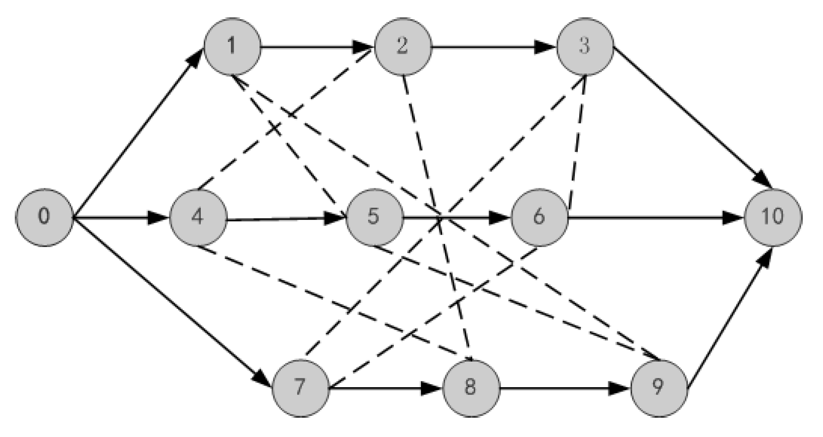
4.1. The JSSP Model
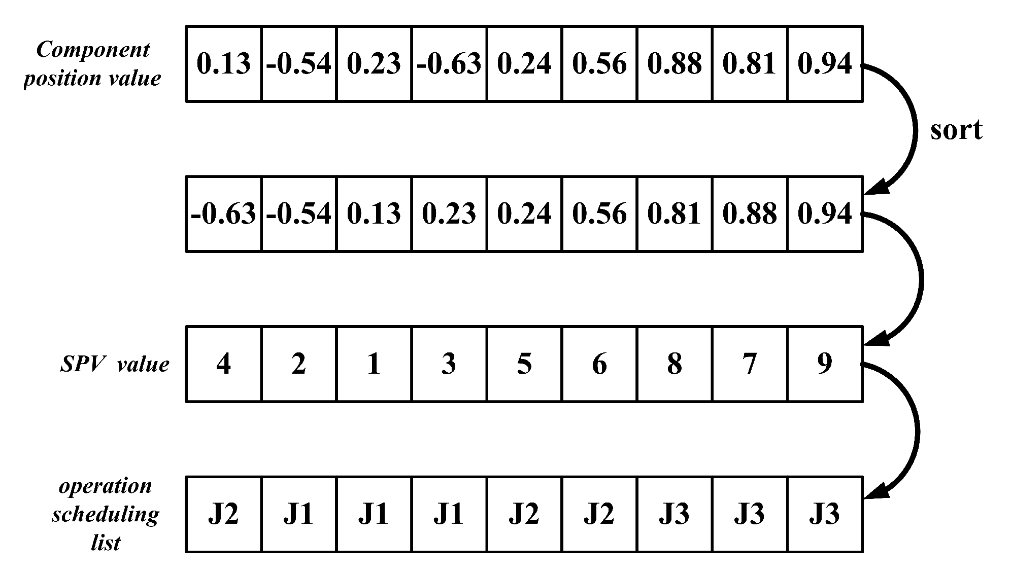
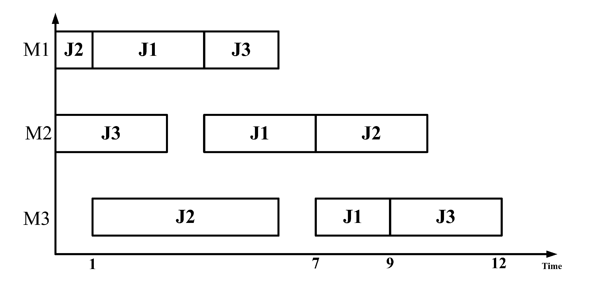
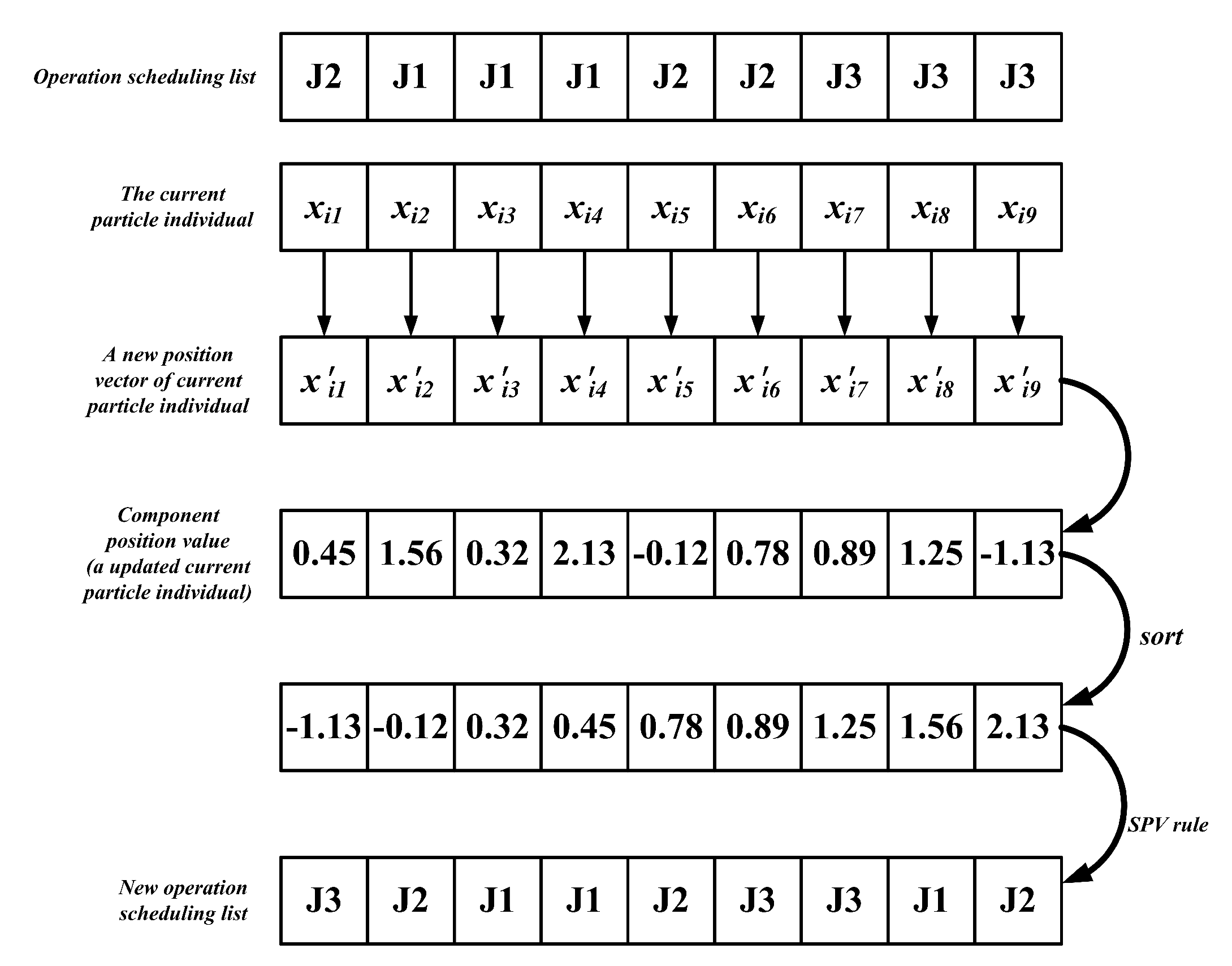
4.2. Analysis of the Main Process of the NGPSO in Solving JSSP
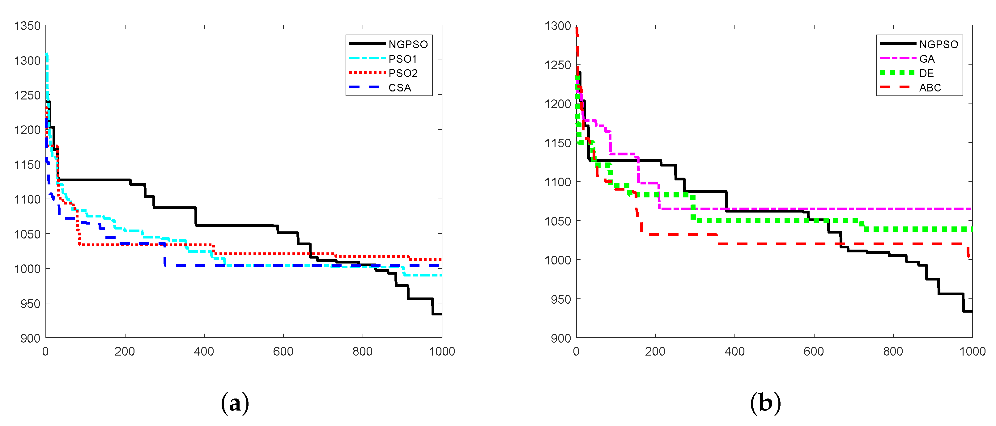
5. Experimental Results and Analysis
6. Conclusions
Author Contributions
Funding
Acknowledgments
Conflicts of Interest
References
- Garey, M.R.; Johnson, D.S.; Sethi, R. The complexity of flowshop and jobshop scheduling. Math. Oper. Res. 1976, 1, 117–129. [Google Scholar] [CrossRef]
- Carlier, J.; EPinson, E. An algorithm for solving the job-shop problem. Manag. Sci. 1989, 35, 164–176. [Google Scholar] [CrossRef]
- Moosavi, E.; Gholamnejad, J.; Ataeepour, M.; Khorram, E. Improvement of lagrangian relaxation performance for open pit mines constrained long-term production scheduling problem. J. Cent. South Univ. 2014, 21, 2848–2856. [Google Scholar] [CrossRef]
- Li, H.; Womer, N.K. Solving stochastic resource-constrained project scheduling problems by closed-loop approximate dynamic programming. Eur. J. Oper. Res. 2015, 246, 20–33. [Google Scholar] [CrossRef]
- Asadzadeh, L. A parallel artificial bee colony algorithm for the job shop scheduling problem with a dynamic migration strategy. Comput. Ind. Eng. 2016, 102, 359–367. [Google Scholar] [CrossRef]
- Yurtkuran, A.; Emel, E. A discrete artificial bee colony algorithm for single machine scheduling problems. Int. J. Prod. Res. 2016, 54, 6860–6878. [Google Scholar] [CrossRef]
- Murugesan, R.; Balan, K.S.; Kumar, V.N. Clonal selection algorithm using improved initialization for solving JSSP. Int. Conf. Commun. Control Comput. Technol. 2010, 470–475. [Google Scholar] [CrossRef]
- Lu, H.; Yang, J. An improved clonal selection algorithm for job shop scheduling. Ubiquitous Comput. 2009, 34–37. [Google Scholar] [CrossRef]
- Hui, T.; Dongxiao, N. Combining simulate anneal algorithm with support vector regression to forecast wind speed. Nternational Conf. Geosci. Remote Sens. 2010, 2, 92–94. [Google Scholar]
- Croce, F.D.; Tadei, R.; Volta, G. A genetic algorithm for the job shop problem. Comput. Oper. Res. 1995, 22, 15–24. [Google Scholar] [CrossRef]
- Wang, L.; Zheng, D.Z. A modified genetic algorithm for job shop scheduling. Int. J. Adv. Manuf. Technol. 2002, 20, 72–76. [Google Scholar] [CrossRef]
- Salido, M.A.; Escamilla, J.; Giret, A.; Barber, F. A genetic algorithm for energy-efficiency in job-shop scheduling. Int. J. Adv. Manuf. Technol. 2016, 85, 1303–1314. [Google Scholar] [CrossRef]
- Zhang, R.; Chiong, R. Solving the energy-efficient job shop scheduling problem: A multi-objective genetic algorithm with enhanced local search for minimizing the total weighted tardiness and total energy consumption. J. Clean. Prod. 2016, 112, 3361–3375. [Google Scholar] [CrossRef]
- Zhonghua, H.; Boqiu, Z.; Hao, L.; Wei, G. Bat algorithm for flexible flow shop scheduling with variable processing time. Int. Conf. Mechatron. 2017, 690, 164–171. [Google Scholar]
- Abdelbasset, M.; Manogaran, G.; Elshahat, D.; Mirjalili, S. A hybrid whale optimization algorithm based on local search strategy for the permutation flow shop scheduling problem. Future Gener. Comput. Syst. 2018, 85, 129–145. [Google Scholar] [CrossRef] [Green Version]
- Simon, D. Biogeography-based optimization. IEEE Trans. Evol. Comput. 2008, 12, 702–713. [Google Scholar] [CrossRef] [Green Version]
- Rahmati, S.H.A.; Zandieh, M. A new Biogeography-Based Optimization (BBO) algorithm for the flexible job shop scheduling problem. Int. J. Adv. Manuf. Technol. 2012, 58, 1115–1129. [Google Scholar] [CrossRef]
- Xinyu, S.; Weiqi, L.; Qiong, L.; Chaoyong, Z. Hybrid discrete particle swarm optimization for multi-objective flexible job-shop scheduling problem. Int. J. Adv. Manuf. Technol. 2013, 67, 2885–2901. [Google Scholar]
- Lian, Z.; Jiao, B.; Gu, X. A similar particle swarm optimization algorithm for job-shop scheduling to minimize makespan. Appl. Math. Comput. 2006, 183, 1008–1017. [Google Scholar]
- Niu, Q.; Jiao, B.; Gu, X. Particle swarm optimization combined with genetic operators for job shop scheduling problem with fuzzy processing time. Appl. Math. Comput. 2008, 205, 148–158. [Google Scholar]
- Ponsich, A.; Coello Coello, C.A. A hybrid differential evolution—Tabu search algorithm for the solution of job-shop scheduling problems. Appl. Soft Comput. 2013, 13, 462–474. [Google Scholar] [CrossRef]
- Huang, K.L.; Liao, C.J. Ant colony optimization combined with taboo search for the job shop scheduling problem. Comput. Oper. Res. 2008, 35, 1030–1046. [Google Scholar] [CrossRef]
- Saidimehrabad, M.; Dehnaviarani, S.; Evazabadian, F.; Mahmoodian, V. An Ant Colony Algorithm (ACA) for solving the new integrated model of job shop scheduling and conflict-free routing of AGVs. Comput. Ind. Eng. 2015, 86, 2–13. [Google Scholar] [CrossRef]
- Zhang, S.J.; Gu, X.S. An effective discrete artificial bee colony algorithm for flow shop scheduling problem with intermediate buffers. J. Cent. South Univ. 2015, 22, 3471–3484. [Google Scholar] [CrossRef]
- Wang, X.; Duan, H. A hybrid biogeography-based optimization algorithm for job shop scheduling problem. Comput. Ind. Eng. 2014, 73, 96–114. [Google Scholar] [CrossRef]
- Lu, Y.; Jiang, T. Bi-population based discrete bat algorithm for the low-carbon job shop scheduling problem. IEEE Access 2019, 7, 14513–14522. [Google Scholar] [CrossRef]
- Rohaninejad, M.; Kheirkhah, A.S.; Vahedi Nouri, B.; Fattahi, P. Two hybrid tabu search–frefly algorithms for the capacitated job shop scheduling problem with sequence-dependent setup cost. Int. J. Comput. Integr. Manuf. 2015, 28, 470–487. [Google Scholar] [CrossRef]
- Babukartik, R.G. Hybrid algorithm using the advantage of ACO and cuckoo search for job scheduling. Int. J. Inf. Technol. Converg. Serv. 2012, 2, 25–34. [Google Scholar] [CrossRef]
- Yu, K.; Wang, X.; Wang, Z. An improved teaching-learning-based optimization algorithm for numerical and engineering optimization problems. J. Intell. Manuf. 2016, 27, 831–843. [Google Scholar] [CrossRef]
- Lu, C.; Xiao, S.; Li, X.; Gao, L. An effective multi-objective discrete grey wolf optimizer for a real-world scheduling problem in welding production. Adv. Eng. Softw. 2016, 99, 161–176. [Google Scholar] [CrossRef] [Green Version]
- Liu, M.; Yao, X.; Li, Y. Hybrid whale optimization algorithm enhanced with lévy flight and differential evolution for job shop scheduling problems. Appl. Soft Comput. J. 2020, 87, 16. [Google Scholar] [CrossRef]
- Sharma, N.; Sharma, H.; Sharma, A. Beer froth artificial bee colony algorithm for job-shop scheduling problem. Appl. Soft Comput. 2018, 68, 507–524. [Google Scholar] [CrossRef]
- Qiu, X.; Lau, H.Y. An AIS-based hybrid algorithm with PSO for job shop scheduling problem. IFAC Proc. Vol. 2010, 43, 350–355. [Google Scholar] [CrossRef]
- Masood, A.; Chen, G.; Mei, Y.; Zhang, M. Reference point adaption method for genetic programming hyper-heuristic in many-objective job shop scheduling. Eur. Conf. Evol. Comput. Comb. Optim. 2018, 116–131. [Google Scholar] [CrossRef]
- Dabah, A.; Bendjoudi, A.; Aitzai, A.; Taboudjemat, N.N. Efficient parallel tabu search for the blocking job shop scheduling problem. Soft Comput. 2019, 23, 13283–13295. [Google Scholar] [CrossRef]
- Zhang, X.; Koshimura, M.; Fujita, H.; Hasegawa, R. An efficient hybrid particle swarm optimization for the job shop scheduling problem. IEEE Int. Conf. Fuzzy Syst. 2011, 622–626. [Google Scholar] [CrossRef]
- Abdel-Kader, R.F. An improved PSO algorithm with genetic and neighborhood-based diversity operators for the job shop scheduling problem. Appl. Artif. Intell. 2018, 32, 433–462. [Google Scholar] [CrossRef]
- Dao, T.; Pan, T.; Nguyen, T.; Pan, J.S. Parallel bat algorithm for optimizing makespan in job shop scheduling problems. J. Intell. Manuf. 2018, 29, 451–462. [Google Scholar] [CrossRef]
- Jiang, T.; Zhang, C.; Zhu, H.; Gu, J.; Deng, G. Energy-efficient scheduling for a job shop using an improved whale optimization algorithm. Mathematics 2018, 6, 220. [Google Scholar] [CrossRef] [Green Version]
- Eberhart, R.; Kennedy, J. A new optimizer using particle swarm theory. In Proceedings of the Mhs95 Sixth International Symposium on Micro Machine and Human Science, Nagoya, Japan, 4–6 October 1995; IEEE: Piscataway, NJ, USA, 2002. [Google Scholar]
- Pan, F.; Chen, D.; Lu, L. Improved PSO based clustering fusion algorithm for multimedia image data projection. Multimed. Tools Appl. 2019, 79, 1–14. [Google Scholar] [CrossRef]
- Şenel, F.A.; Gökçe, F.; Yüksel, A.S.; Yiğit, T. A novel hybrid PSO–GWO algorithm for optimization problems. Eng. Comput. 2018, 20, 1359–1373. [Google Scholar] [CrossRef]
- Yang, X. Swarm intelligence based algorithms: A critical analysis. Evol. Intell. 2014, 7, 17–28. [Google Scholar] [CrossRef] [Green Version]
- Ostadmohammadi Arani, B.; Mirzabeygi, P.; Shariat Panahi, M. An improved PSO algorithm with a territorial diversity-preserving scheme and enhanced exploration–exploitation balance. Swarm Evol. Comput. 2013, 11, 1–15. [Google Scholar] [CrossRef]
- Rezaei, F.; Safavi, H.R. GuASPSO: A new approach to hold a better exploration–exploitation balance in PSO algorithm. Soft Comput. 2020, 24, 4855–4875. [Google Scholar] [CrossRef]
- Deepa, O.; Senthilkumar, A. Swarm intelligence from natural to artificial systems: Ant colony optimization. Int. J. Appl. Graph Theory Wirel. Ad Hoc Netw. Sens. Netw. 2016, 8, 9–17. [Google Scholar]
- Zuo, X.; Zhang, G.; Tan, W. Self-adaptive learning PSO-based deadline constrained task scheduling for hybrid iaas cloud. IEEE Trans. Autom. Ence Eng. 2014, 11, 564–573. [Google Scholar] [CrossRef]
- Chen, S.M.; Chiou, C.H. Multiattribute decision making based on interval-valued intuitionistic fuzzy sets, PSO techniques, and evidential reasoning methodology. IEEE Trans. Fuzzy Syst. 2015, 23, 1905–1916. [Google Scholar] [CrossRef]
- Chen, S.M.; Jian, W.S. Fuzzy forecasting based on two-fctors second-order fuzzy-tend logical relationship groups, similarity measures and PSO techniques. Inf. Sci. 2016, 391, 65–79. [Google Scholar]
- Wang, X.W.; Yan, Y.X.; Gu, X.S. Welding robot path planning based on levy-PSO. Kongzhi Yu Juece Control Decis. 2017, 32, 373–377. [Google Scholar]
- Godio, A.; Santilano, A. On the optimization of electromagnetic geophysical data: Application of the PSO algorithm. J. Appl. Geophys. 2018, 148, 163–174. [Google Scholar] [CrossRef]
- Khan, I.; Pal, S.; Maiti, M.K. A hybrid PSO-GA algorithm for traveling salesman problems in different environments. Int. J. Uncertain. Fuzziness Knowl. Based Syst. 2019, 27, 693–717. [Google Scholar] [CrossRef]
- Lu, L.; Luo, Q.; Liu, J.; Wu, X. An improved particle swarm optimization algorithm. Granul. Comput. 2008, 193, 486–490. [Google Scholar]
- Qin, Q.; Cheng, S.; Zhang, Q.; Li, L.; Shi, Y. Biomimicry of parasitic behavior in a coevolutionary particle swarm optimization algorithm for global optimization. Appl. Soft Comput. 2015, 32, 224–240. [Google Scholar] [CrossRef]
- Hema, C.R.; Paulraj, M.P.; Yaacob, S.; Adom, A.H.; Nagarajan, R. Functional link PSO neural ntwork based classification of EEG mental task signals. Int. Symp. Inf. Technol. 2008, 3, 1–6. [Google Scholar]
- Rao, A.R.; Sivasubramanian, K. Multi-objective optimal design of fuzzy logic controller using a self configurable dwarm intelligence algorithm. Comput. Struct. 2008, 86, 2141–2154. [Google Scholar]
- Pan, Q.; Tasgetiren, M.F.; Liang, Y. A discrete particle swarm optimization algorithm for single machine total earliness and tardiness problem with a common due date. IEEE Int. Conf. Evol. Comput. 2006, 3281–3288. [Google Scholar] [CrossRef]
- Lin, L.; Gen, M. Auto-tuning strategy for evolutionary algorithms: Balancing btween exploration and exploitation. Soft Comput. 2009, 13, 157–168. [Google Scholar] [CrossRef]
- Crepinsek, M.; Liu, S.H.; Mernik, M. Exploration and exploitation in evolutionary algorithms: A survey. ACM Comput. Surv. 2013, 45, 1–35. [Google Scholar] [CrossRef]
- Zhao, Z.; Zhang, G.; Bing, Z. Job-shop scheduling optimization design based on an improved GA. World Congr. Intell. Control Autom. 2012, 654–659. [Google Scholar] [CrossRef]
- Zhu, L.J.; Yao, Y.; Postolache, M. Projection methods with linesearch technique for pseudomonotone equilibrium problems and fixed point problems. U.P.B. Sci. Bull. Ser. A. 2020. In press. [Google Scholar]
- Fan, S.S.; Chiu, Y. A decreasing inertia weight particle swarm optimizer. Eng. Optim. 2007, 39, 203–228. [Google Scholar] [CrossRef]
- El Sehiemy, R.A.; Selim, F.; Bentouati, B.; Abido, M.A. A Novel multi-objective hybrid particle swarm and salp optimization algorithm for technical-economical-environmental operation in power systems. Energy 2019, 193, 116817. [Google Scholar] [CrossRef]
- Shi, Y.H.; Eberhart, R.C.; Shi, Y.; Eberhart, R.C. Empirical study of particle swarm optimization. Congr. Evol. Comput. 1999, 3, 101–106. [Google Scholar]
- Krohling, R.A. Gaussian particle swarm with jumps. Congr. Evol. Comput. 2005, 2, 1226–1231. [Google Scholar]
- Wiech, J.; Eremeyev, V.A.; Giorgio, I. Virtual spring damper method for nonholonomic robotic swarm self-organization and leader following. Contin. Mech. Thermodyn. 2018, 30, 1091–1102. [Google Scholar] [CrossRef] [Green Version]
- Yao, X.; Liu, Y.; Lin, G. Evolutionary programming made faster. IEEE Trans. Evol. Comput. 1999, 3, 82–102. [Google Scholar]
- Yu, S. Differential evolution quantum particle swarm optimization for solving job-shop scheduling problem. In Chinese Control and Cecision Conference; IEEE: Piscataway, NJ, USA, 2019. [Google Scholar]
- Zhu, Z.; Zhou, X. An efficient evolutionary grey wolf optimizer for multi-objective flexible job shop scheduling problem with hierarchical job precedence constraints. Comput. Ind. Eng. 2020, 140, 106280. [Google Scholar] [CrossRef]
- Song, X.; Chang, C.; Zhang, F. A novel parallel hybrid algorithms for job shop problem. Int. Conf. Nat. Comput. 2008, 452–456. [Google Scholar] [CrossRef]
- Song, X.; Chang, C.; Cao, Y. New particle swarm algorithm for job shop scheduling problems. World Congr. Intell. Control Autom. 2008, 3996–4001. [Google Scholar] [CrossRef]
- Wang, L.; Tang, D. An improved adaptive genetic algorithm based on hormone modulation mechanism for job-shop scheduling problem. Expert Syst. Appl. 2011, 38, 7243–7250. [Google Scholar] [CrossRef]
- Tasgetiren, M.F.; Sevkli, M.; Liang, Y.-C.; Gençyilmaz, G. Particle swarm optimization algorithm for single machine total weighted tardiness problem. Evol. Comput. 2004, 2, 1412–1419. [Google Scholar]
- Rao, Y.; Meng, R.; Zha, J.; Xu, X. Bi-objective mathematical model and improved algorithm for optimisation of welding sop scheduling problem. Int. J. Prod. Res. 2019, 58, 2767–2783. [Google Scholar] [CrossRef]
- Ling, W. Jop Shop Scheduling Problems and Genetic Algorithm; Tsinghua University Press: Beijing, China, 2003; pp. 59–63. (In Chinese) [Google Scholar]
- Meng, Q.; Zhang, L.; Fan, Y. A hybrid particle swarm optimization algorithm for solving job shop scheduling problems. In Theory, Methodology, Tools and Applications for Modeling and Simulation of Complex Systems; Springer: Singapore, 2016; pp. 71–78. [Google Scholar]


| Dimension | 1 | 2 | 3 | 4 | 5 | 6 |
|---|---|---|---|---|---|---|
| position value | 0.36 | 0.01 | 0.67 | 0.69 | 1.19 | 1.02 |
| smallest position value | 2 | 1 | 3 | 4 | 6 | 5 |
| Projects | Jobs | Operations Number | ||
|---|---|---|---|---|
| 1 | 2 | 3 | ||
| J1 | 3 | 3 | 2 | |
| operation time | J2 | 1 | 5 | 3 |
| J3 | 3 | 2 | 3 | |
| J1 | M1 | M2 | M3 | |
| machine sequence | J2 | M1 | M3 | M2 |
| J3 | M2 | M1 | M3 | |
| Instance | OVCK | NGPSO | PSO-NIW | PSO-GM | PSO | ||||||||
|---|---|---|---|---|---|---|---|---|---|---|---|---|---|
| Best | Worst | Avg | Best | Worst | Avg | Best | Worst | Avg | Best | Worst | Avg | ||
| FT06 | 55 | 55 | 55 | 55 | 55 | 55 | 55 | 55 | 55 | 55 | 55 | 55 | 55 |
| FT10 | 930 | 930 | 1056 | 955 | 930 | 1118 | 967 | 930 | 1073 | 959 | 932 | 1149 | 977 |
| FT20 | 1165 | 1210 | 1311 | 1247 | 1178 | 1253 | 1249 | 1167 | 1313 | 1256 | 1180 | 1274 | 1261 |
| LA1 | 666 | 666 | 666 | 666 | 666 | 666 | 666 | 666 | 666 | 666 | 666 | 666 | 666 |
| LA2 | 655 | 655 | 655 | 655 | 655 | 655 | 655 | 655 | 655 | 655 | 655 | 655 | 655 |
| LA3 | 597 | 597 | 676 | 635 | 597 | 680 | 539 | 609 | 679 | 646 | 624 | 690 | 653 |
| LA4 | 590 | 590 | 622 | 609 | 613 | 646 | 627 | 604 | 635 | 618 | 627 | 678 | 634 |
| LA5 | 593 | 593 | 593 | 593 | 593 | 593 | 593 | 593 | 593 | 593 | 593 | 593 | 593 |
| LA6 | 926 | 926 | 926 | 926 | 926 | 926 | 926 | 926 | 926 | 926 | 926 | 926 | 926 |
| LA7 | 890 | 890 | 890 | 890 | 890 | 890 | 890 | 890 | 890 | 890 | 890 | 890 | 890 |
| LA8 | 863 | 863 | 863 | 863 | 863 | 863 | 863 | 863 | 863 | 863 | 863 | 863 | 863 |
| LA9 | 951 | 951 | 951 | 951 | 951 | 951 | 951 | 951 | 951 | 951 | 951 | 951 | 951 |
| LA10 | 958 | 958 | 997 | 969 | 963 | 1053 | 998 | 958 | 1022 | 988 | 958 | 1069 | 999 |
| LA11 | 1222 | 1222 | 1222 | 1222 | 1222 | 1222 | 1222 | 1222 | 1222 | 1222 | 1222 | 1222 | 1222 |
| LA12 | 1039 | 1039 | 1039 | 1039 | 1039 | 1039 | 1039 | 1039 | 1039 | 1039 | 1039 | 1039 | 1039 |
| LA13 | 1150 | 1150 | 1150 | 1150 | 1150 | 1150 | 1150 | 1150 | 1150 | 1150 | 1150 | 1150 | 1150 |
| LA14 | 1292 | 1292 | 1292 | 1292 | 1292 | 1292 | 1292 | 1292 | 1292 | 1292 | 1292 | 1292 | 1292 |
| LA15 | 1207 | 1207 | 1207 | 1207 | 1207 | 1207 | 1207 | 1207 | 1207 | 1207 | 1207 | 1207 | 1207 |
| LA16 | 945 | 945 | 945 | 945 | 945 | 992 | 978 | 945 | 972 | 956 | 962 | 994 | 980 |
| LA17 | 784 | 794 | 803 | 798 | 811 | 878 | 849 | 784 | 866 | 833 | 822 | 879 | 836 |
| LA18 | 848 | 848 | 999 | 913 | 848 | 1033 | 924 | 848 | 1054 | 933 | 857 | 1088 | 957 |
| LA19 | 842 | 842 | 1032 | 905 | 889 | 1087 | 923 | 878 | 1073 | 933 | 891 | 1131 | 946 |
| LA20 | 902 | 908 | 1228 | 965 | 1113 | 1342 | 1127 | 1009 | 1304 | 1130 | 1152 | 1385 | 1223 |
| LA21 | 1046 | 1183 | 1271 | 1208 | 1190 | 1318 | 1224 | 1046 | 1324 | 1230 | 1201 | 1398 | 1244 |
| LA22 | 927 | 927 | 989 | 966 | 936 | 1014 | 979 | 927 | 1112 | 982 | 957 | 1194 | 992 |
| LA23 | 1032 | 1032 | 1245 | 1123 | 1109 | 1299 | 1203 | 1097 | 1283 | 1196 | 1100 | 1307 | 1208 |
| LA24 | 935 | 968 | 1153 | 983 | 998 | 1184 | 1076 | 935 | 1166 | 1047 | 1003 | 1182 | 1089 |
| LA25 | 977 | 977 | 1089 | 994 | 987 | 1145 | 1018 | 980 | 1129 | 1007 | 991 | 1211 | 1014 |
| LA26 | 1218 | 1218 | 1443 | 1311 | 1233 | 1489 | 1383 | 1226 | 1442 | 1362 | 1287 | 1459 | 1399 |
| LA27 | 1235 | 1394 | 1476 | 1412 | 1423 | 1499 | 1445 | 1403 | 1478 | 1431 | 1396 | 1503 | 1477 |
| LA28 | 1216 | 1216 | 1440 | 1381 | 1230 | 1457 | 1390 | 1219 | 1444 | 1387 | 1290 | 1445 | 1379 |
| LA29 | 1152 | 1280 | 1397 | 1304 | 1310 | 1429 | 1339 | 1344 | 1450 | 1410 | 1339 | 1557 | 1412 |
| LA30 | 1355 | 1335 | 1567 | 1417 | 1404 | 1620 | 1503 | 1396 | 1592 | 1500 | 1428 | 1701 | 1511 |
| Instance | OVCK | NGPSO | PSO1 | PSO2 | CSA | ||||||||
|---|---|---|---|---|---|---|---|---|---|---|---|---|---|
| Best | Worst | Avg | Best | Worst | Avg | Best | Worst | Avg | Best | Worst | Avg | ||
| ABZ5 | 1234 | 1234 | 1457 | 1311 | 1234 | 1466 | 1323 | 1287 | 1487 | 1344 | 1234 | 1583 | 1447 |
| ABZ6 | 943 | 943 | 1219 | 1093 | 943 | 1223 | 1137 | 954 | 1235 | 1120 | 1004 | 1284 | 1121 |
| ABZ7 | 656 | 713 | 997 | 862 | 689 | 1087 | 901 | 664 | 1176 | 925 | 985 | 1329 | 1150 |
| ABZ8 | 665 | 729 | 1298 | 1031 | 819 | 1470 | 1285 | 927 | 1483 | 1232 | 1199 | 1589 | 1337 |
| ABZ9 | 679 | 930 | 1015 | 976 | 985 | 1024 | 990 | 958 | 1016 | 982 | 1008 | 1079 | 1034 |
| ORB1 | 1059 | 1174 | 1297 | 1226 | 1214 | 1317 | 1276 | 1177 | 1282 | 1235 | 1232 | 1374 | 1353 |
| ORB2 | 888 | 913 | 1038 | 957 | 969 | 1074 | 989 | 943 | 1010 | 970 | 1022 | 1114 | 1070 |
| ORB3 | 1005 | 1104 | 1243 | 1172 | 1144 | 1265 | 1181 | 1166 | 1270 | 1192 | 1228 | 1295 | 1267 |
| ORB4 | 1005 | 1005 | 1163 | 1140 | 1005 | 1182 | 1066 | 1016 | 1167 | 1078 | 1046 | 1211 | 1132 |
| ORB5 | 887 | 887 | 1002 | 987 | 887 | 1028 | 994 | 913 | 1013 | 988 | 877 | 1092 | 997 |
| ORB6 | 1010 | 1124 | 1203 | 1170 | 1187 | 1245 | 1221 | 1171 | 1247 | 1213 | 1191 | 1265 | 1222 |
| ORB7 | 397 | 397 | 464 | 440 | 435 | 468 | 447 | 397 | 468 | 441 | 458 | 482 | 460 |
| ORB8 | 899 | 1020 | 1106 | 1054 | 1018 | 1163 | 1056 | 899 | 1155 | 1080 | 1073 | 1173 | 1085 |
| ORB9 | 934 | 980 | 1128 | 1032 | 1012 | 1139 | 1043 | 1021 | 1154 | 1042 | 1011 | 1150 | 1032 |
| ORB10 | 944 | 1027 | 1157 | 1048 | 1040 | 1143 | 1067 | 1036 | 1154 | 1063 | 944 | 1204 | 1097 |
| LA31 | 1784 | 1784 | 2143 | 1972 | 1784 | 2149 | 1986 | 1849 | 2156 | 1961 | 1872 | 2212 | 2057 |
| LA32 | 1850 | 1850 | 2202 | 1987 | 1850 | 2237 | 1996 | 1944 | 2248 | 2002 | 1982 | 2397 | 2123 |
| LA33 | 1719 | 1719 | 2001 | 1894 | 1719 | 2035 | 1907 | 1719 | 2022 | 1897 | 1829 | 2155 | 1956 |
| LA34 | 1721 | 1721 | 2060 | 1939 | 1878 | 2147 | 1963 | 1721 | 2126 | 1955 | 2060 | 2304 | 2187 |
| LA35 | 1888 | 1888 | 2212 | 1986 | 1888 | 2271 | 2010 | 1930 | 2308 | 2039 | 1918 | 2431 | 2181 |
| LA36 | 1268 | 1408 | 1665 | 1523 | 1396 | 1691 | 1545 | 1415 | 1703 | 1562 | 1511 | 1775 | 1660 |
| LA37 | 1397 | 1515 | 1693 | 1560 | 1524 | 1792 | 1623 | 1551 | 1787 | 1635 | 1613 | 1805 | 1743 |
| LA38 | 1196 | 1196 | 1596 | 1388 | 1332 | 1781 | 1569 | 1198 | 1610 | 1454 | 1483 | 1708 | 1624 |
| LA39 | 1233 | 1662 | 1799 | 1701 | 1712 | 1725 | 1718 | 1711 | 1825 | 1748 | 1731 | 1833 | 1768 |
| LA40 | 1222 | 1222 | 1537 | 1413 | 1289 | 1583 | 1425 | 1244 | 1615 | 1423 | 1453 | 1661 | 1528 |
| YN1 | 888 | 1248 | 1346 | 1291 | 1303 | 1411 | 1346 | 1259 | 1395 | 1289 | 1291 | 1426 | 1318 |
| YN2 | 909 | 911 | 1208 | 1102 | 927 | 1198 | 1109 | 932 | 1226 | 1117 | 1042 | 1318 | 1207 |
| YN3 | 893 | 893 | 1376 | 1189 | 903 | 1344 | 1201 | 893 | 1457 | 1255 | 1003 | 1487 | 1311 |
| YN4 | 968 | 984 | 1299 | 1106 | 979 | 1376 | 1137 | 1008 | 1410 | 1124 | 1153 | 1677 | 1329 |
| Instance | OVCK | NGPSO | GA | DE | ABC | ||||||||
|---|---|---|---|---|---|---|---|---|---|---|---|---|---|
| Best | Worst | Avg | Best | Worst | Avg | Best | Worst | Avg | Best | Worst | Avg | ||
| ABZ5 | 1234 | 1234 | 1457 | 1311 | 1234 | 1460 | 1336 | 1234 | 1465 | 1347 | 1236 | 1572 | 1443 |
| ABZ6 | 943 | 943 | 1219 | 1093 | 954 | 1247 | 1142 | 948 | 1179 | 1103 | 992 | 1285 | 1138 |
| ABZ7 | 656 | 713 | 997 | 862 | 729 | 1128 | 927 | 720 | 1166 | 918 | 973 | 1239 | 1106 |
| ABZ8 | 665 | 729 | 1298 | 1031 | 805 | 1386 | 1242 | 822 | 1384 | 1165 | 748 | 1314 | 1137 |
| ABZ9 | 679 | 930 | 1015 | 976 | 988 | 1124 | 1003 | 926 | 1023 | 988 | 944 | 1052 | 989 |
| ORB1 | 1059 | 1174 | 1297 | 1226 | 1210 | 1348 | 1296 | 1191 | 1302 | 1244 | 1213 | 1320 | 1306 |
| ORB2 | 888 | 913 | 1038 | 957 | 958 | 1064 | 997 | 932 | 1125 | 965 | 947 | 1096 | 988 |
| ORB3 | 1005 | 1104 | 1243 | 1172 | 1136 | 1273 | 1201 | 1154 | 1281 | 1203 | 1228 | 1295 | 1267 |
| ORB4 | 1005 | 1005 | 1163 | 1140 | 1005 | 1178 | 1057 | 1005 | 1183 | 1135 | 1005 | 1239 | 1142 |
| ORB5 | 887 | 887 | 1002 | 987 | 913 | 1125 | 1006 | 887 | 1046 | 994 | 877 | 1092 | 1017 |
| ORB6 | 1010 | 1124 | 1203 | 1170 | 1187 | 1349 | 1227 | 1171 | 1247 | 1213 | 1194 | 1277 | 1236 |
| ORB7 | 397 | 397 | 464 | 440 | 397 | 479 | 456 | 397 | 468 | 441 | 397 | 471 | 455 |
| ORB8 | 899 | 1020 | 1106 | 1054 | 1038 | 1188 | 1068 | 899 | 1149 | 1067 | 1043 | 1164 | 1076 |
| ORB9 | 934 | 980 | 1128 | 1032 | 997 | 1158 | 1042 | 1003 | 1184 | 1055 | 1011 | 1150 | 1032 |
| ORB10 | 944 | 1027 | 1157 | 1048 | 1024 | 1242 | 1107 | 1026 | 1163 | 1059 | 944 | 1164 | 1147 |
| LA31 | 1784 | 1784 | 2143 | 1972 | 1784 | 2216 | 1978 | 1784 | 2177 | 1978 | 1784 | 2241 | 2078 |
| LA32 | 1850 | 1850 | 2202 | 1987 | 1862 | 2249 | 2003 | 1935 | 2250 | 2013 | 1903 | 2344 | 2013 |
| LA33 | 1719 | 1719 | 2001 | 1894 | 1786 | 2126 | 1923 | 1719 | 2103 | 1914 | 1749 | 2052 | 1948 |
| LA34 | 1721 | 1721 | 2060 | 1939 | 1889 | 2155 | 1972 | 1721 | 2140 | 1953 | 1764 | 2054 | 1962 |
| LA35 | 1888 | 1888 | 2212 | 1986 | 1888 | 2310 | 2015 | 1926 | 2319 | 2044 | 1902 | 2332 | 2135 |
| LA36 | 1268 | 1408 | 1665 | 1523 | 1416 | 1631 | 1566 | 1423 | 1698 | 1557 | 1411 | 1765 | 1650 |
| LA37 | 1397 | 1515 | 1693 | 1560 | 1549 | 1812 | 1647 | 1544 | 1767 | 1628 | 1524 | 1783 | 1646 |
| LA38 | 1196 | 1196 | 1596 | 1388 | 1211 | 1682 | 1467 | 1214 | 1607 | 1450 | 1196 | 1609 | 1425 |
| LA39 | 1233 | 1662 | 1799 | 1701 | 1677 | 1831 | 1782 | 1688 | 1845 | 1732 | 1681 | 1840 | 1746 |
| LA40 | 1222 | 1222 | 1537 | 1413 | 1263 | 1602 | 1438 | 1255 | 1602 | 1431 | 1257 | 1610 | 1424 |
| YN1 | 888 | 1248 | 1346 | 1291 | 1288 | 1430 | 1351 | 1260 | 1419 | 1292 | 1288 | 1419 | 1306 |
| YN2 | 909 | 911 | 1208 | 1102 | 934 | 1201 | 1116 | 946 | 1240 | 1125 | 979 | 1253 | 1126 |
| YN3 | 893 | 893 | 1376 | 1189 | 914 | 1355 | 1212 | 893 | 1387 | 1262 | 904 | 1422 | 1218 |
| YN4 | 968 | 984 | 1299 | 1106 | 993 | 1384 | 1149 | 993 | 1426 | 1133 | 1082 | 1327 | 1129 |
© 2020 by the authors. Licensee MDPI, Basel, Switzerland. This article is an open access article distributed under the terms and conditions of the Creative Commons Attribution (CC BY) license (http://creativecommons.org/licenses/by/4.0/).
Share and Cite
Yu, H.; Gao, Y.; Wang, L.; Meng, J. A Hybrid Particle Swarm Optimization Algorithm Enhanced with Nonlinear Inertial Weight and Gaussian Mutation for Job Shop Scheduling Problems. Mathematics 2020, 8, 1355. https://doi.org/10.3390/math8081355
Yu H, Gao Y, Wang L, Meng J. A Hybrid Particle Swarm Optimization Algorithm Enhanced with Nonlinear Inertial Weight and Gaussian Mutation for Job Shop Scheduling Problems. Mathematics. 2020; 8(8):1355. https://doi.org/10.3390/math8081355
Chicago/Turabian StyleYu, Hongli, Yuelin Gao, Le Wang, and Jiangtao Meng. 2020. "A Hybrid Particle Swarm Optimization Algorithm Enhanced with Nonlinear Inertial Weight and Gaussian Mutation for Job Shop Scheduling Problems" Mathematics 8, no. 8: 1355. https://doi.org/10.3390/math8081355