Numerical Investigation on Generation and Propagation Characteristics of Offshore Tsunami Wave under Landslide


1
Haikou Marine Geological Survey Center, China Geological Survey, Haikou 570100, China
2
Hubei Key Laboratory of Marine Geological Resources, China University of Geosciences, Wuhan 430074, China
3
Shandong Provincial Key Laboratory of Ocean Engineering, Ocean University of China, Qingdao 266100, China
*
Author to whom correspondence should be addressed.
Appl. Sci. 2020, 10(16), 5579; https://doi.org/10.3390/app10165579
Submission received: 6 July 2020
/
Revised: 4 August 2020
/
Accepted: 10 August 2020
/
Published: 12 August 2020
(This article belongs to the Special Issue Numerical Simulation of the Tsunami Propagation)
Abstract
:Tsunamis induced by the landslide will divide into a traveling wave component propagating along the coastline and an offshore wave component propagating perpendicular to the coastline. The offshore tsunami wave has the non-negligible energy and destruction in enclosed basins as fjords, reservoirs, and lakes, which are worth studying. The initial submergence condition, the falling height and sliding angle of slider, are important reference indexes of damage degree of landslide and may also matter at that of the landslide-induced tsunami. Depending on the fully coupled model, the effects of them on the production and propagation of the tsunami were considered in the study. Since the slider used was semi-elliptic, the effect of the ratio of the long axis to the short axis was also analyzed. According to the computational fluid dynamics theory, a numerical wave tank was developed by the immersed boundary (IB) method; besides, the general moving-object module of slide mass was also embedded to the numerical tanker. The results indicate that the effects of the squeezing and pushing of the slider on water produce a naturally attenuated wave at the front of the wave train, and the attenuation becomes more serious with the increase in the initial submersion range of the slider. The effects of the vertical movement of the slider cause the increase in the amplitude of the back of the wave train. As the falling height increases, the large wave height increases when the slider is initially submerged and decreases when it is not initially submerged, except for the accidental elevation of that at smaller falling heights. The results also indicate that the hazard of the subaerial landslide-induced tsunami is greater under a small or large falling angle, and that of the partial subaerial and submarine landslide-induced tsunami is greater under a small falling angle. With the increase in the ratio of the long axis to the short axis, the total induced wave energy decreases and the shape of the wave train proportionally reduces, while the wave propagation mode does not change.
1. Introduction
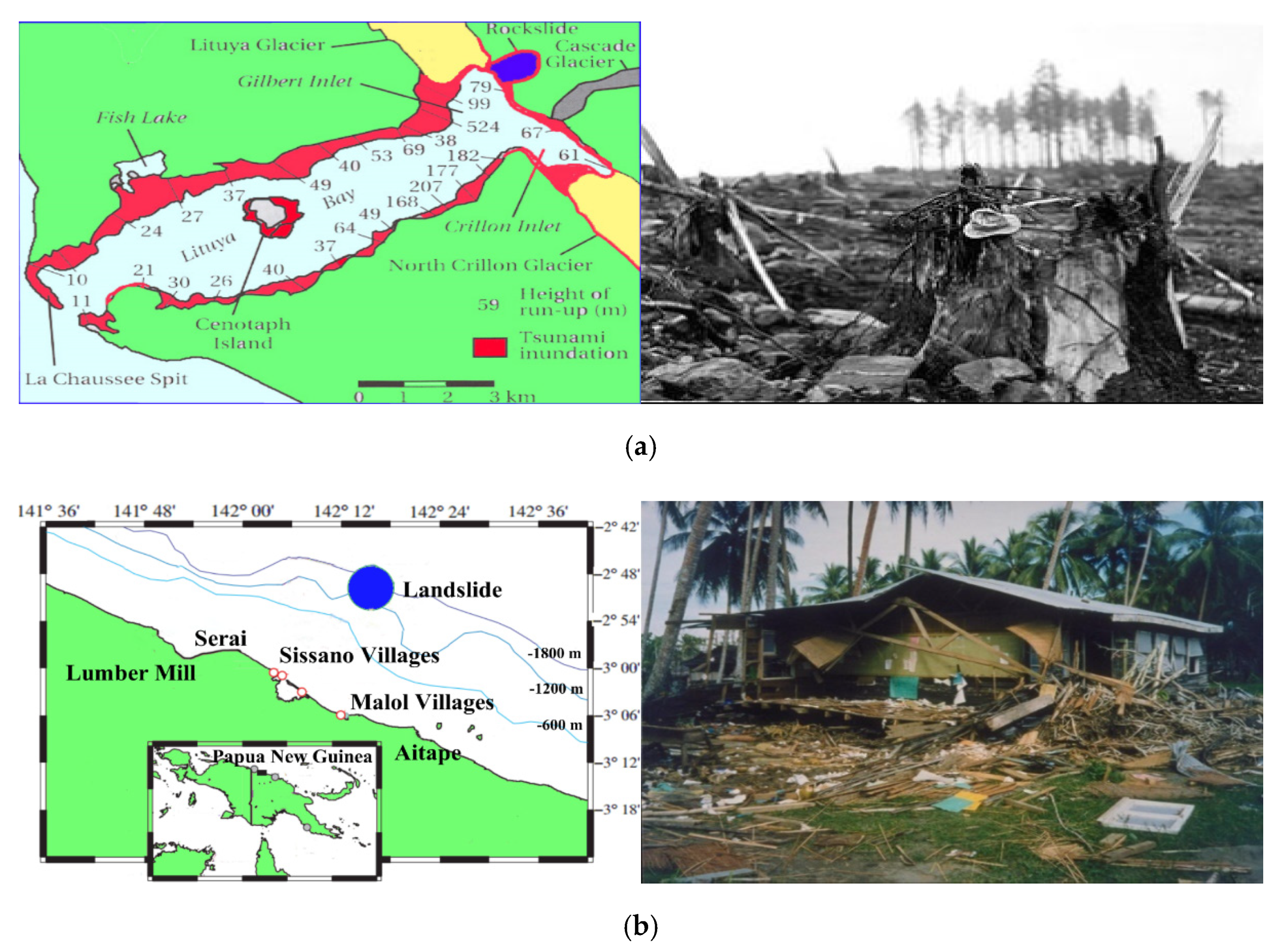
It is generally believed that tsunamis can be divided into landslide-induced tsunamis and earthquake-induced tsunamis according to their causes. Due to the long duration and large spread distance of the earthquake-induced tsunami, it causes massive disasters, such as the Indian Ocean tsunami on 26 December 2004 and the Indonesian tsunami on 17 July 2006. Some large-volume landslide-induced tsunami has the same magnitude of long run-out as earthquake-induced tsunami and also causes substantial regional impact [1,2]. By contrast, landslide-induced tsunamis have three distinctive characteristics: larger run-ups locally, delayed time of arrival and the focusing of inundation along a narrow coastline, which means that it can cause locally larger disasters than the earthquake-induced tsunamis [3,4]. For example, the Lituya Bay tsunami (9 July 1958), the largest tsunami ever recorded, produced a run-up in excess of 400 m. In fact, after the Lituya Bay tsunami, there was another tsunami that caused great damage locally. It was the Papua New Guinea (PNG) tsunami, which was caused by an underwater landslide of a total volume of 6.4 km3 and resulted in a 15 m run-up and 2000 deaths [5]. These two landslides-induced tsunamis have attracted the attention of the international tsunami organization and a large number of researchers. Until today, some research results and understandings related to the generation and propagation of tsunami waves have been obtained. The relevant information and the damage of the Lituya Bay tsunami and the PNG tsunami are in Figure 1.
The tsunami caused by landslides can be divided into three types according to the initial submerged status of the slide block (submarine, subaerial, partial subaerial). The submarine landslides, which have less moving material in total but 100 times in vertically moving distance compared to the earthquakes, have caused the same comparable and damaging tsunami [6]. For example, the 1998 Papua New Guinea [4,7], the 1992 Flores Island [8]. In general, landslides in deep water areas are subcritical. Tsunamis caused by such landslides usually do not accumulate heavily, but run away from the landslide center. Bondevik et al. 2005 further studied the wave patterns caused by subcritical landslides and found that a free surface drop would occur where the slider enters the water, followed by a symmetric sickle-shaped free surface [1]. Løvholt et al. 2005 also studied the tsunami characteristics caused by subcritical landslides, and found that, under strong subcritical conditions, the maximum free surface elevation increased with the increase in landslide volume and slide acceleration, and decreased with the increase in slide velocity, while the uplifted water volume was in direct proportion to the landslide volume and Froude number [9]. For the submarine landslide-induced tsunami in the shallow water area, higher and sharper waves are usually formed due to the slower wave velocity and higher Froude number. Tsunami spread caused by the submarine landslides with rapid acceleration or deceleration has a common characteristic which is the frequency dispersion; for example, the Tsunami generated by the Papua New Guinea Landslide in 1998 [7,10]. The importance of dispersion was also demonstrated in some studies [11,12], which found that there was at least a 50% relative error of a non-dispersion model in the maximum free surface elevation simulation compared with the dispersion model.
Subaerial landslide-induced tsunami is also a research hotspot [13,14]. Tinti et al., 2005 gives a detailed description of the initial stage of landslide tsunami, and mainly discovering that, when the sliding block enters the water, it will squeeze the water and push the water forward, forming an offshore wave that spreads attenuating to the far field. At the same time, a depression appears where the shoreline retreats and will result in a significant stress gradient. Affected by these pressure gradient forces, a massive amount of water poured into the depression and rebounded to form two traveling waves propagating along the coastline [15]. Sammarco and Renzi systematically studied the generation and propagation characteristics of landslide-induced tsunamis from 2008 to 2012. The study in 2008 found that the large amplitude waves did not appear in the front of the wave list, but in the middle, which was different from the earthquake-induced tsunami and caused great disaster in the early stage, when people did not know much about the landslide-induced tsunami [16]. The 2010 study of Renzi and Sammarco found that traveling waves around the conical islands do not travel completely along the coastline and are partly free from the constraints of the circular coastline, but still have run-up [17]. They found in 2012 that irregular landslide geometry could lead to sharp twin peaks of waves and that the continental shelf could reduce the severity of the tsunami [18].
However, most studies in the past have focused on traveling waves, and few have studied the generation and propagation of offshore waves. An in-depth study of this part is necessary. Because, on the one hand, the amplitude of an offshore wave as it travels from the near field to the far field does not decay as quickly as earlier studies suggested [19,20]. This suggests that, in the limited near field and the part of far field, offshore waves actually have non-negligible energy and destruction, especially in enclosed basins (to as fjords, reservoirs, and lakes), which were seriously underestimated in the past study [13]. On the other hand, in the path of offshore wave propagation to the far-field, there are usually some important offshore structures, such as submarine pipelines, risers, cross-sea Bridges, and offshore platforms, which will lead to huge economic losses and environmental pollution if they are damaged. In order to protect these important structures, it is necessary to study the characteristics of the generation and propagation of near-sea waves and their interactions with these structures. In addition to ignoring the importance of studying the near-sea waves, most past research has focused on a single initial inundation condition [21,22]. Few studies have investigated and compared the effects of the three different initial submersion conditions (submarine, subaerial, and partial subaerial) on tsunamis, and few studies have explained the differences in the characteristics of the generation and propagation of the three landslide tsunamis.
In this paper, considering the importance of the vertical physics acceleration in the initial stage of the landslide-induced tsunami [23,24,25] and the importance of the whole development process of the landslide [26], the general moving-object module and hydrodynamic and turbulence module are coupled to numerically simulate the production and propagation of landslide-induced tsunamis, which compares the physical experiment to verify the model. Through a large number of simulation cases with different settings, this paper analyzes the characteristics of the generation and propagation of offshore waves and studies the influence of different initial submergence conditions of sliders (submarine, subaerial, and partial subaerial). In addition, the effects of sliding height, sliding angle and slider geometry on landslide-induced tsunami are also studied. The rest of the paper is organized as follows. The second Section introduces the numerical simulation methods and equations. The verification of this model is conducted in the third Section. The systematic simulations are carried out in the fourth Section where the effects of the different initial submergence conditions, sliding heights, sliding angles and slider geometry are analyzed. The conclusions of this work and prospects for the future are given in the fifth Section.
2. Numerical Methods
In the numerical model, the flow and slide mass are coupled by the immersed boundary (IB) method. The mesh of the calculation domain is subdivided into the fixed rectangular cells. The numerical fixed slope and slide mass are fully coupled in the fluid domain by defining the fractional volumes of the objects to cells [27]. In this model, the true volume-of-fluid (VOF) method is used to calculate the free surface motion [28]. The Reynolds-Averaged Navier–Stokes Equations and incompressible flow continuity equation are solved to calculate the fluid flow. The general moving-object module, together with the vertical physical acceleration, is used to simulate the interaction between the moving object and the fluid to reproduce the wave process generated by the landslide.
2.1. Hydrodynamic and Turbulence Module
In this model, the renormalization-group (RNG) k-ε turbulence model was implemented as the turbulence closure, which has been successfully employed to investigate the turbulence field around the structure and the whole computational domain under the interaction between structure and water [29,30]. The volume of fluid (VOF) method was used to capture the interface between the air and water [31,32,33], and the pressure and velocity was coupled by the generalized minimal residual methods (GMRES) pressure-velocity solvers. In the free surface flow, the mass and momentum conservation equations in the flow can be expressed as
where ∇ is a gradient operator; V is the velocity vector; S is the area fraction of the fluid in the system grid in Cartesian coordinate; F is the volume fraction of the fluid (the percentage of the fluid volume to the volume of a single cell). ρ is the fluid density, p is the pressure, Aobjet and Aflow are acceleration vector of object and viscous acceleration vector of flow, respectively.
According to the volume of fluid (VOF) method, the transportation equation of the free surface between water and air is formulated as
where f is the water volume fraction in the cell of a free surface. f = 1, 0 < f < 1, and f = 0 represent the different phases of water, interface and air, respectively.
The viscous acceleration vector of flow Aflow in the three directions of the Cartesian coordinate can be written as
where str (I = x, y, z) is the wall stress in three directions and included in an implicit way to avoid the possible numerical instabilities arising in cells with large wall areas and small flow volumes. The basic approach for the Vz (z direction velocity) equation, for example, is as follows. Wall shears influencing Vz can arise from the wall areas located on x or y cell faces surrounding Vz. For any one of these faces, if the fractional flow area S is less than a unity, the remaining area fraction (1 − S) is considered to be a wall on which a stress is generated. On an 𝑥 face to the right of Vz, for instance, the acceleration due to wall shear in laminar flow, strz, is an approximation to ∂/∂x (μ (∂Vz/∂x)):
where Sx, δx (the cell size) and μ (the viscosity at the cell center) are evaluated in the cell in which Vz is located. The area fraction Sz is estimated at the same control volume face where Vz is located. The velocity Vz0 is either zero or is equal to the z direction tangential velocity at the moving component and mesh boundaries. Because Vz is on the boundary between the two cells, the Sx is an average for these cells. Similar stresses are evaluated at each of the four surrounding cell walls, and their sum is taken as the total stress.
For turbulent shear stress, the formula of strz changes to:
where Vx * is the local shear velocity. The quadratic expression for the tangential velocity is linearized, with the Vz in the parenthesis on the right-hand side taken at time level n + 1.
The terms of shear stress are calculated as
To calculate the turbulent viscosity u, two-equation κ-ε turbulence model is introduced as
where k is the turbulent kinetic energy; ε is turbulent energy dissipation rate; Vx, Vy and Vz are the velocities in x, y, and z directions; Prot is the turbulent kinetic energy production; Tbuoyancy,t is the buoyancy production term; Tdiffusion and Tdiffusion,ε demonstrate diffusion terms and C1ε, C2ε and C3ε are constant values, respectively.
2.2. General Moving-Object Module
The area and volume fractions are recalculated at each time step, according to the updated position and direction of the object. In the module, the collision is assumed to be instantaneous and is allowed to occur between the fixed slope and the slider as well as between the slider and the wall of the computational domain. The collision is completely plastic.
According to the kinematics, the general motion of the slider can be divided into translational motion and rotational motion. The velocity at any point on the slider (P) is equal to the velocity at the geometric center point of the slider (G) due to no rotation occurring in this model. The velocity relationship can be expressed as
where the VP represents the velocity at any point on the slider, and VG represents the velocity at the geometric center on the slider. Equation of motion governing is:
where the F is the total force including the gravity, supporting force and friction in the air, and the extra buoyancy and the flow resistance in the water, m is the mass of the slider. The flow resistance can be written as
where the D is the drag force, L is the lift force, CD and CL are the drag coefficient and lift coefficient, respectively, and B is the area of incoming flow.
The effects of volume and area fractions of slider on incompressible fluid flow are considered. The general form of the continuity equation can be written as
where Vf and A are the volume and area fractions of the slider, respectively; Vcell is volume of a mesh cell; Sobj, n and Vobj are, respectively, the surface area, unit normal vector and the velocity of the moving object in the mesh cell.
3. Model Validation
3.1. Model Setup
Since this paper mainly analyzes the generation and propagation characteristics of landslide-induced tsunami waves, it is very important to verify the calculation accuracy of our numerical model in predicting the wave and flow induced by the landslide and simulating wave attenuation propagation depending on the comparisons between numerical and physical results. The experiments were conducted by Romano et al. (2016) to obtain the free surface elevation time series collected using the movable system at three angular positions and four radial distances [28]. The scale of 1:1 is used in numerically simulating the physical experiment carried by Romano et al. 2016. The numerical experimental layout based on Romano et al. (2016) is displayed in Figure 2.
The length, height, and still water depth of the numerical wave tank are 20, 2, and 0.8 m, respectively. The mesh resolution in the slider zone is 0.001 m. The origin of the coordinate system is defined at the bottom of the numerical flume. The slope angle () is kept constant at (i.e., one vertical and three horizontal) in the numerical verification example. The size and angle of the slope will change with the setting of other examples to ensure that the slider will slide normally on the slope and fall into the water. Due to only the offshore wave generation and propagation being considered in the numerical simulation, the conical islands in the physical experiment are simplified as flat beaches and the sliders are simplified as rectangles in the cross-section. The long axis b, width c and short axis a of the slider in the numerical verification example are 0.8, 0.134 and 0.05 m, respectively. The slider long axis and short axis will change without changing the total volume when the influence of slider geometry is discussed. The volume of the slider is controlled at 0.0084152 m3, with a relative error of 0.18% compared to 0.0084 m3 in the physics experiment. The density of the slider is a constant of 1833.33 kg/m3. Seven wave sensors are located behind the slope to measure the temporal elevation of the wave surface profiles, and their distance from the undisturbed shoreline are (S1: r = 0.23 m; S2: r = 0.38 m; S3: r = 0.53 m; S4: r = 0.73 m; S5: r = 1.03 m; S6: r = 1.43 m; S7: r = 1.83 m), which is the same as the sensor position in the physics experiments. Two additional wave gauges are added to the numerical simulation to study the characteristics of wave propagation and the locations are (G1: x = 2 m, G2: x = 4 m). The friction coefficient of both the slider and the slope is 0.206, which is consistent with the physics experiments in Romano et al. (2016). In the simulation, the vertical distance from the lowest point of the slider to the seabed is , and the initial is 0.94 m. The still water depth is 0.8 m. When the numerical verification experiment begins, the slider is released and moves towards the still water surface. Replace the velocities of the fluid in the x and z direction at the center of the cell with the average velocities of the fluid flowing through the cell in the x and z direction. The TECPLOT post-processing software is then used to calculate the total flow rate of the fluid and color the values to form the velocity cloud diagram. Figure 3 depicts the velocity cloud diagram when the slider enters the water and when the slider is completely immersed.
3.2. Model Validation
As shown in Figure 3b, the front of the slide block extrudes a crest when it enters the water and the maximum velocity appears on the front edge and surface of the landslide, as well as the surface of the crest. As shown in Figure 3a, when the slide block is completely submerged, the flow velocity on the middle surface of the slide block decreases and the high-speed flow area appears on the rear edge of the landslide except for the leading edge. At the same time, there was a depression near the shoreline with the high-speed flow area moving from the crest to the trough, which means that a massive amount of water was poured into this depression. The development process of landslide-induced tsunami is consistent with that described in previous studies [16], which can well demonstrate the accuracy of the numerical model in predicting the wave and flow induced by the landslide. Figure 4 depicts the temporal evolution of water elevation between the simulation and experiment results at the locations of S1, S3, S4 and S5. The measured and computational results about the wave peak and its temporal variation are generally in good agreement [28], which can well demonstrate the accuracy of the numerical model in simulating wave attenuation propagation.
4. Results and Discussions
In the following sections, the effects of the slider with different falling heights, different falling angles and different slider geometries are investigated to reveal the wave generation and propagation characteristics of the tsunami wave and the interaction mechanism between the wave and the landslide. The impacts of three different initial submergence conditions (submarine, subaerial, and partial subaerial) are discussed in detail in each set of experiments. The slope angle () changes with the setting of the falling angles. The slider long axis and short axis change with the setting of the slider geometries but without changing the total volume. The ratio of the long axis to the short axis of the slider is R. The vertical distance from the lowest point of the slider to the seabed is which changes with the setting of the falling heights, The volume of the slider is controlled at 0.0084152 m3 and the density of the slider is a constant of 1833.33 kg/m3. The friction coefficient of both the slider and the slope is 0.206. The mesh resolution around the landslide is 0.002 m and the total number of cells is 1.5 million. Two wave gauges (G1 and G2) are located at the r = 2 and 4 m from the undisturbed shoreline to monitor the changes in the water level before and after the slider comes to move. Table 1 lists the parameter setup for all simulation runs.
4.1. Effect of Falling Height under Different Submergence Conditions
In this section, the effects of the falling heights with different submergence conditions on the landslide-induced tsunami are investigated. The long axis b, short axis a and width c of the slider are 0.8, 0.134 and 0.05 m, respectively. According to the initial submerged state of the slide block, the landslide is divided into subaerial landslides, partial subaerial landslides and submarine landslides. Each of the different landslides were used to simulate the landslide-induced tsunamis at six different falling heights. The slope angle was fixed at 18.43 and the depth of the still water was 0.8 m. The schematic diagram of setups is displayed in Figure 5.
4.1.1. Cases of Subaerial Landslides
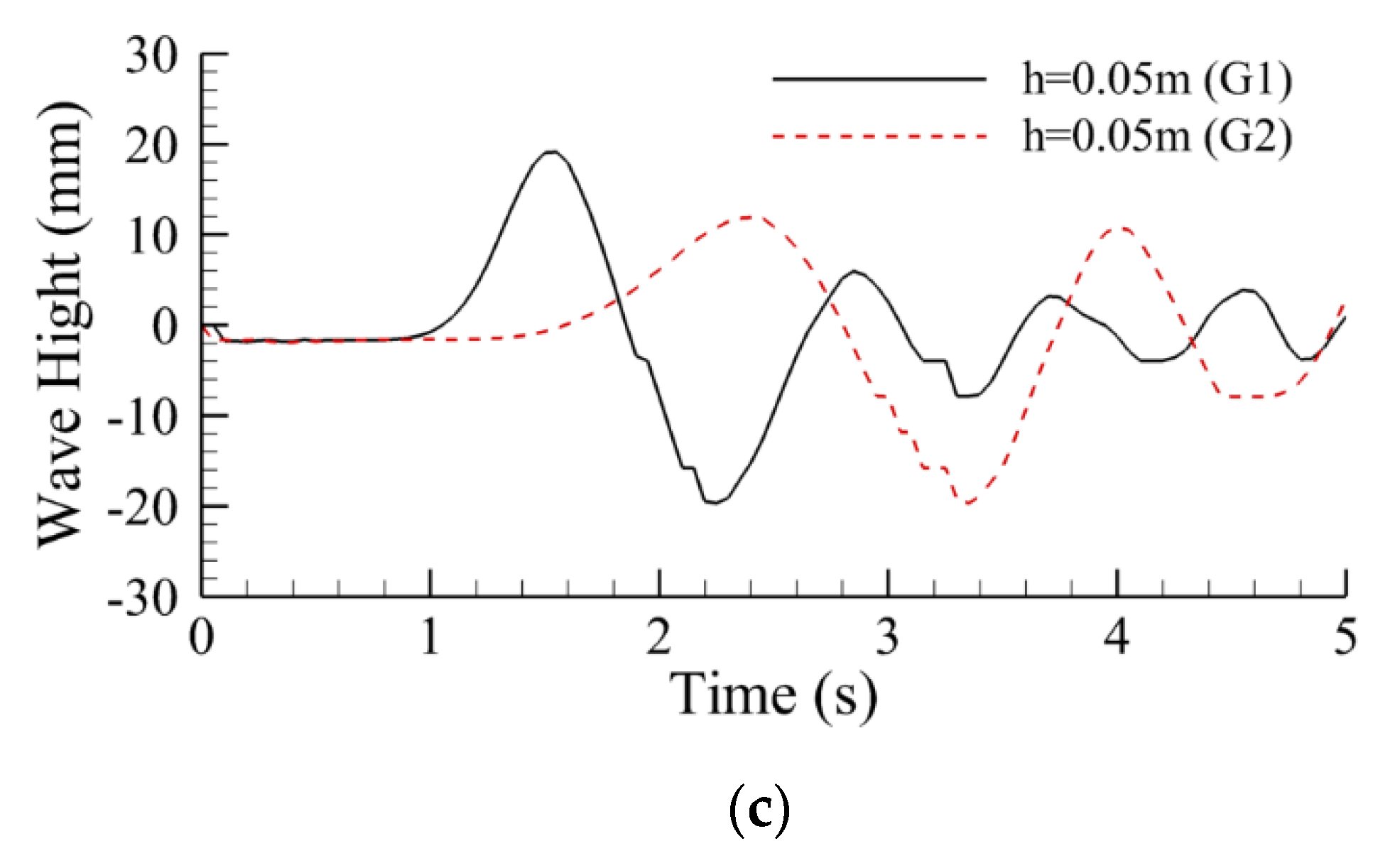
The falling heights (h) refer to the vertical distance between the initial lowest point of the slider and the still water surface, which are set as 0.05, 0.1, 0.15, 0.2, 0.25 and 0.3, respectively, and the submergence condition of landslide is a subaerial landslide. When the falling heights (h) are 0.05, 0.15 and 0.25 m, the temporal evolution of the water elevation in the G1 and G2 point are shown in Figure 6. The first crest in the wave list of the offshore component of the landslide-induced tsunami is attenuated when propagating from G1 to G2 (from the solid lines to the dotted lines in Figure 6), but the second crest in the wave train is not attenuated or even increased (Figure 6). Because, on the one hand, the first crest of the wave train is caused by squeezing and pushing the shallow water as the slider enters the water. After the slider completely enters the water, the extrusion effect moves from the shallow water to the deep water, which leads to the fact that after the first crest is generated, there is no new energy input and only energy dissipation. On the other hand, the second crest of the wave train is caused by water pouring into the depression. When the slider completely enters the water, there will still be a pressure gradient above the trailing edge of the moving slider, causing the water to move downward and rebound upward, which means that the second crest will be affected by the water moving above the trailing edge of the slider in the process of propagation. With energy input during propagation, the second crest is larger at G2 than at G1. Similarly, the first trough of the wave train is also affected by the change of flow field caused by the slider, so the attenuation is not obvious when propagating from G1 to G2 (from the solid lines to dotted lines in Figure 6).
4.1.2. Cases of Partial Subaerial Landslides
The falling heights (h) are set as −0.05, −0.1, −0.15, −0.2, −0.25 and −0.3, respectively, and the submergence conditions of the landslides are partial subaerial landslides. When the falling heights (h) are −0.05, −0.15 and −0.25 m, the temporal evolution of the water elevation in G1 and G2 point are shown in Figure 7. Compared with Figure 6, the overall law of the tsunami wave train caused by subaerial landslide does not vary with the falling height, while that caused by the partial subaerial landslide will change with the decrease in the falling height. Specifically, from h = −0.05 m to h = −0.25 m, the initial submerged range of the slider becomes larger, and the gap between the first and second peak of the wave train decreases until the second peak exceeds the first peak and becomes the new highest peak in the wave train. However, in fact, in terms of value, only the first crest of the wave train decreases while the second crest does not change significantly, which leads to the phenomenon that the gap between the two is reduced, or even that the latter is reversed. This indicates that when the slider is initially submerged, the squeezing and pushing effect of the initial slider motion on the water decreases and decreases more with the increase in the initial submerged area. It can be seen from Figure 7 that the effect of the slider movement on the first trough and the second peak are weakened during the propagation process with the increases in the initial submersion range of the slider. Specifically, the amplitude of the second peak and the first trough propagating to G2 decreases as the initial submersion range of the slider increases.
4.1.3. Cases of Submarine Landslides
The falling heights (h) are set as −0.3, −0.35, −0.4, −0.45, −0.5 and −0.55, respectively, and the submergence conditions of the landslides are submarine landslides. When the falling heights (h) are −0.35, −0.45 and −0.55 m, the temporal evolution of water elevation in the G1 and G2 points are shown in Figure 8. With the decrease in the falling height, the mode of tsunami wave train caused by the submarine landslide becomes more and more complicated and is no longer a regular oscillation mode, and when h = −0.55 m, the wave height increases unexpectedly at 4.2 s. The overall tsunami amplitude caused by the submarine landslides is smaller than that of the subaerial and partial subaerial landslides, of course, in the case of that the landslide volume is the same. In reality, the scope and volume of the submarine landslides are often larger than that of the subaerial and partial subaerial landslides, which leads to the fact that submarine landslides can also cause extremely harmful tsunamis. Submarine landslides usually occur with earthquakes, so in theory, they can occur anywhere in the ocean, rather than just near the coast. When submarine landslides occur on continental slopes or continental bases, the depth of the landslide is large, but the initial wave amplitude is not large, and it is difficult to detect on the sea surface. The large ratio of the wave length to wave height, the extremely fast propagation speed and the imperceptibility of such tsunamis often lead to huge disasters.
4.1.4. Effect of Falling Heights
Six different falling heights were calculated for each initial submergence condition, for a total of 18 cases. The change of maximum wave height with falling height is shown in Figure 9. The maximum wave heights measured at G1 are marked as the solid lines in Figure 9 and that at G2 are marked as the dotted lines. The triangle, square and circle, respectively, represent the subaerial landslide, partial subaerial landslide and submarine landslide in Figure 9. It is worth noting that, in general, the tsunami wave height of the partial subaerial landslide is the largest, followed by that of the subaerial landslide, and the smallest is that of the submarine landslide. However, when the falling height of the submarine landslides is less than −0.5 m, the maximum wave height at G2 is close to that of partial subaerial landslides and even slightly exceeds that of subaerial landslides. The variation of maximum wave height caused by the subaerial landslide with the falling height of the slide block is relatively simple, that is, the greater the falling height, the smaller the maximum wave height. This phenomenon is reflected in many reservoir landslides, and there is an optimal falling height range within which landslides cause the maximum surge height. On the contrary, generally speaking, the maximum wave height caused by a submarine landslide and partial subaerial landslides increases with the increase in initial falling height of the slide block, except for the accidental elevation of submarine landslide-induced tsunamis at smaller falling heights. When the tsunami wave propagates from G1 to G2 (from the solid lines to dotted lines in Figure 9), the attenuation phenomenon of the maximum wave height of subaerial landslide has no significant change, while that of the partial subaerial landslide will be reduced with the increase in initial submersion range. For submarine landslides, the attenuation phenomenon almost disappeared when the initial falling height was higher. However, when the initial falling height is small (h = −0.4 m ~−0.6 m), the maximum wave height of the wave train increases unexpectedly during the propagation. This unexpected increase in wave height may be due to the fact that the landslide occurs in deep sea area and the landslide disturbs the high-pressure seawater while the upper low-pressure seawater is less affected. Then, with the propagation of the tsunami, the disturbed high-pressure seawater from the lower layer is gradually released to the upper layer and affects the upper layer of the seawater. As a result, in the beginning, the wave height of the tsunami is small because the surface water is less disturbed and then increases because the effect of the disturbed high-pressure seawater.
4.2. Effect of Falling Angle under Different Submergence Conditions
In this section, the effects of the falling angles with different submergence conditions on the landslide-induced tsunami are investigated. The long axis b, short axis a and width c of the slider are 0.8, 0.134 and 0.05 m respectively. According to the initial submerged state of the slide block, the landslide is divided into subaerial landslide, partial subaerial landslide and submarine landslide. Each of the different landslides is used to simulate the landslide-induced tsunami at six different falling angles. The of subaerial landslide, partial subaerial landslide and submarine landslide are fixed at 0.8, 0.6 and 0.4 m, and the initial falling heights of them are 0, −0.2 and −0.4 m, respectively. The depth of the still water was 0.8 m. The schematic diagram of setups is displayed in Figure 10.
4.2.1. Cases of Subaerial Landslides
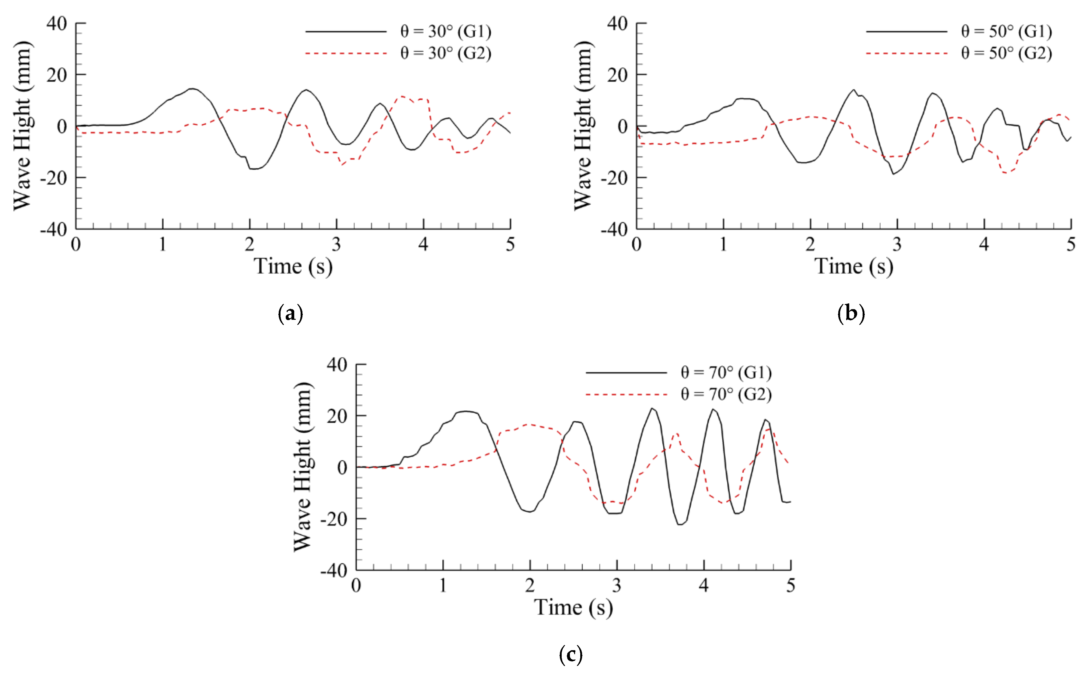
The falling angles () refer to the angle between the sliding direction of the slider along the slope and the positive x direction and are set as 20, 30, 40, 50, 60 and 70, respectively, and the submergence conditions of the landslides are subaerial landslide (the falling height is 0 m). When the falling angles are 30, 50 and 70, the temporal evolution of water elevation in the G1 and G2 point are shown in Figure 11. The most obvious wave propagation feature is that the oscillation at the back of the wave train intensifies as the falling angle increases at G1. Specifically, there has been a significant attenuation of the fluctuation between 4 and 5 s at 30 at the back of the wave list, which diminishes at 50, and almost disappears at 70 (each wave has almost the same large amplitude in the entire wave train at 70). This continuous large amplitude wave train caused by the sliding block falling with a large angle has serious perniciousness. Compared with G1, the most obvious propagation feature at G2 is attenuation, as the initial falling height of the slider is 0 m, which can also be reflected in Figure 9. It is worth noting that the maximum wave heights at G1 and G2 do not simply vary linearly with the falling angle. The maximum wave heights of 30 and 50 are basically the same and the maximum wave height of 70 is greater than either of them, which indicated that there is a complex pattern in the effect of falling angle on the generation and propagation of tsunami waves. This pattern will be discussed later in conjunction with the change of maximum falling angles with falling height.
4.2.2. Cases of Partial Subaerial Landslides
The falling angles () refer to the angle between the sliding direction of the slider along the slope and the positive x direction, and are set as 20, 30, 40, 50, 60 and 70, respectively, and the submergence conditions of landslides are partial subaerial landslides (the falling height is −0.2 m). When the falling angles are 30, 50 and 70, the temporal evolution of water elevation in the G1 and G2 point are shown in Figure 12. Similar to the case of subaerial landslide, the oscillation amplitude of partial subaerial landslide-induced wave behind the wave train at G1 increases with the increase in falling angle, and the significant attenuation of the fluctuation also existed at G2. Different from subaerial landslides, the wave train amplitude of partial subaerial landslide-induced wave at G1 and G2 are generally smaller than that of subaerial landslide-induced waves, which, of course, is also related to the smaller initial falling height of partial subaerial landslides. The other particular thing is that the maximum amplitude of G1 at 30, 50 and 70 is not significantly different (only slightly reduced at 70 compared with 30 and 50), which is completely different from subaerial landslides. Compared to the maximum amplitude at G1, there is a slightly noticeable attenuation of that at G2 with the increase in the falling angle. This pattern of maximum amplitude variation is quite different from that of subaerial landslides and will be discussed later in conjunction with the change of maximum falling angles with falling height.
4.2.3. Cases of Submarine Landslides
The falling angles () refer to the angle between the sliding direction of the slider along the slope and the positive x direction, and are set as 20, 30, 40, 50, 60 and 70, respectively, and the submergence conditions of the landslides are submarine landslides (the falling height is −0.4 m). When the falling angles are 30, 50 and 70, the temporal evolution of water elevation in the G1 and G2 point is shown in Figure 13. The front part of the wave train at G1 decays significantly and the rear part decays first and then slightly increases as the falling angle increases. Specifically, the first peak, the second peak and the first trough in the front of the wave train can be identified at 30. When the falling angle is 50, the first peak is almost gone and the second peak and the first trough are reduced in amplitude. The two peaks and the first trough are already very small at 70. Compared to the G1, the front and rear part of the wave list at G2 are both attenuated significantly as the falling angle increases, which suggests that, for underwater landslides near the continental shelf, an increased falling angle would reduce the tsunami hazard because the slide stays on the continental shelf earlier and the slide continuing to slide at a small angle would cause greater harm.
4.2.4. Effect of Falling Angles
Six different falling angles were calculated for each initial submergence condition, for a total of 18 cases. The change of maximum wave height with falling height is shown in Figure 14. The maximum wave heights measured at G1 are marked as the solid lines in Figure 14 and that at G2 are marked as dotted lines. The triangle, square and circle, respectively, represent the subaerial landslide, partial subaerial landslide and submarine landslide in Figure 14. It can be seen that as the falling angle increases, the maximum wave height of the tsunami caused by the subaerial landslide first decreases and then increases, and the maximum wave height difference between G1 and G2 first increases and then decreases, among which the turning point is about 45. This indicates that, for the subaerial landslide-induced tsunami, the horizontal movement of the slider is the dominant factor that causes the tsunami when the falling angle is small (below 45) by squeezing and pushing the water horizontally. As the falling angle of the slider increases from 20 to 45, although the horizontal acceleration component of gravity of the slider increases, that of the flow resistance increases more intensely due to the increase in the area of horizontal incoming flow (Bx), which causes the total horizontal acceleration of the slider to decrease. This decrease in the total horizontal acceleration component and the decrease in horizontal movement distance result in the attenuation of the horizontal influence of the slider on the water and the decrease in the maximum wave height. When the falling angle exceeds 45, the vertical acceleration component becomes the main component of the slider motion, and the influence of the vertical motion of the slider on the wave is dominant. As the falling angle of the slider increases from 45 to 70, the vertical acceleration component of the gravity of the slider increases, that of the flow resistance decreases due to the decrease in the area of vertical incoming flow (Bz), which causes the total horizontal acceleration of the slider to increase. The maximum wave increases due to the increase in the total vertical acceleration of the slider. Of course, this is only the qualitative analysis, while quantitative analysis requires many formulae derivations and experimental data to verify, which will be further studied in future work. In addition, the critical angle does not have to be 45, which also needs further research. However, when the initial submersion condition of the slider is partial submersion and complete submersion, the situation changes. Specifically, the maximum wave height of the partial subaerial and submarine landslide-induced tsunamis will still decrease as the falling angle increases (increasing but not exceeding 45) but the increase in the maximum wave height after 45 is not obvious to them. In other words, the hazard of the subaerial landslide-induced tsunami is greater under a small or large falling angle and that of the partial subaerial and submarine landslide-induced tsunami is greater under a small falling angle.
4.3. Effect of Slider Geometry under Different Submergence Conditions
In this section, the effects of the slider geometry with different submergence conditions on the landslide-induced tsunami were investigated. The width c of the slider is 0.134 m and the ratio of the long axis to the short axis of the slider (R) is from 6 to 16. According to the initial submerged state of the slide block, the landslides are divided into subaerial landslides, partial subaerial landslides and submarine landslides. Each of the different landslides is used to simulate the landslide-induced tsunami at six different R. The of the subaerial landslide, partial subaerial landslide and submarine landslide are fixed at 0.8, 0.6 and 0.4 m, respectively, and their initial falling heights are 0, −0.2 and −0.4 m, respectively. The slope angle was fixed at 18.43 and the depth of still water was 0.8 m. The schematic diagram of setups is displayed in Figure 15.
4.3.1. Cases of Subaerial Landslides
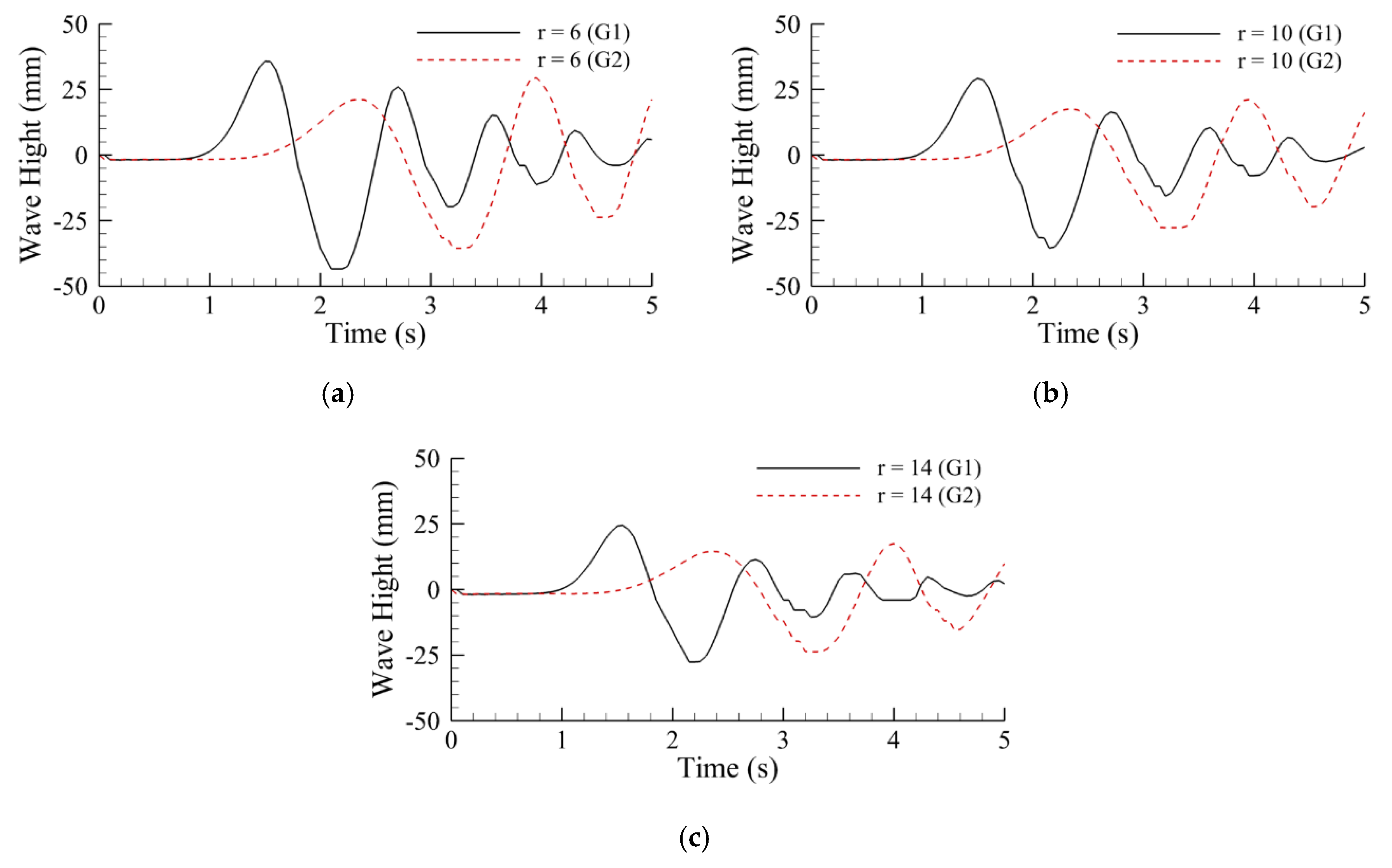
The ratio of the long axis to the short axis of the slider (R) are set as 6, 8, 10, 12, 14 and 16, respectively, and the submergence conditions of landslides are subaerial landslides (the falling height is 0 m). When the falling angles are 6, 10 and 14, the temporal evolution of water elevation in the G1 and G2 point are shown in Figure 16. The first crest in the wave list of the offshore component of the landslide-induced tsunami is attenuated when propagating from G1 to G2 (from the solid lines to dotted lines in Figure 16), but the second crest in the wave train is not attenuated or even increased (Figure 16). Similarly, the first trough of the wave train has a slight attenuation when propagating from G1 to G2. These patterns of transmission in Figure 16a–c do not change as the ratio changed and the temporal evolution of water elevation in G1 and G2 point is exactly similar in Figure 16a–c. However, with the increase in the ratio, the wave height caused by the subaerial landslide decreases, which means that although the ratio does not change the wave propagation mode, it will reduce the total energy contained in the wave.
4.3.2. Cases of Partial Subaerial Landslides
The ratio of the long axis to the short axis of slider (R) are set as 6, 8, 10, 12, 14 and 16, respectively, and the submergence condition of the landslides is partially subaerial (the falling height is −0.2 m). When the falling angles are 6, 10 and 14, the temporal evolution of water elevation in the G1 and G2 point are shown in Figure 17. When the wave train propagates from G1 to G2 (from the solid lines to the dotted lines in Figure 17), the first peak and the first trough have some attenuation, while the second peak increases. As the ratio increases, the first peak and the second peak in the wave series at G1 decay only slightly. By contrast, that of the first trough decays more sharply as the ratio increases. Similarly, the first crest in the wave train at G2 has some slight attenuation as the ratio increases. However, the second peak and the first trough attenuate obviously when the ratio changes from 6 to 10 and attenuate slightly when the ratio changes from 10 to 14, which indicates that the increase in the ratio has a greater influence on the trough in the wave train than the peak and that on the second peak is greater than the first peak (especially from the 6 and 10 of the ratio).
4.3.3. Cases of Submarine Landslides
The ratio of the long axis to the short axis of slider (R) are set as 6, 8, 10, 12, 14 and 16, respectively, and the submergence condition of the landslides is submarine (the falling height is −0.4 m). When the falling angles are 6, 10 and 14, the temporal evolution of the water elevation in G1 and G2 point are shown in Figure 18. Combining Figure 16, Figure 17 and Figure 18, it can be found that the influence of ratio on wave generation and propagation is the same under the different initial submergence conditions. In summary, firstly, the first peak and the first trough of the wave train attenuate during its propagation (from the solid lines to the dotted lines in Figure 16, Figure 17 and Figure 18), while the second peak increases. Secondly, as the ratio increases, the wave propagation law remains unchanged but the total energy decreases. Specifically, as the ratio increases, the amplitude at G1 or G2 decreases, and the trough decreases more than the peak and the second peak decreases more than the first peak.
4.3.4. Effect of Slider Geometry
Six different R were calculated for each initial submergence condition, for a total of 18 cases. The change of maximum wave height with R is shown in Figure 19. The maximum wave heights measured at G1 are marked as the solid line in Figure 19 and that at G2 are marked as a dotted line. The triangle, square and circle, respectively, represent the subaerial landslide, partial subaerial landslide and submarine landslide in Figure 19. It can be seen that the wave height of the subaerial landslide (h = 0 m) is the largest, followed by the partial subaerial landslide (h = −0.2 m), and that of the submarine landslide (h = −0.4 m) is the smallest, which is consistent with the conclusion proven in Figure 9. As the ratio increases, the maximum wave heights all decrease at the three different initial submerged states at G1 and G2, which indicates that the total wave energy decreases as the ratio increases.
5. Conclusions
In this paper, the generation and propagation of a landslide-induced tsunami with different initial submergence condition were investigated, which consider three aspects. In the first aspect, because the essence of landslide-induced tsunami is that the gravitational potential energy of landslide is converted into wave energy, the effect of falling height with a different initial submergence condition is considered. In the second aspect, due to the different slope angles of landslides in reality, the investigations on the effect of the falling angle of the slider with different initial submergence conditions are conducted. In the third aspect, under different geotechnical characteristics of coasts, the geometry of a landslide is various, therefore, the effect of the ratio of the long axis to the short axis of the slider is also studied. The conclusions of this paper are as follows.
As the slider moves in the water, it squeezes and pushes the water in the horizontal direction, while creating a pressure gradient in the vertical direction causing the water to rush downward and bounce upward. The effects of squeezing and pushing produce a naturally attenuated wave at the front of the wave train. The effects of the vertical moving of the slider cause the increase in the amplitude at the back of the wave train.
- For a subaerial landslide-induced tsunami, the maximum wave height decreases with the increase in the initial falling height, and there is an optimal falling height range within which landslides cause the maximum surge height. For submarine landslides and partial subaerial landslide-induced tsunamis, the maximum wave height increases with the increase in initial falling height, except for the accidental elevation of submarine landslide-induced tsunamis at smaller falling heights. When the slider is initially partially submerged, the attenuation of landslide-induced waves appears in the propagation process, and the attenuation becomes more serious with the increase in the initial submersion range.
- Since there is a greater total horizontal acceleration at a smaller falling angle and a greater total vertical acceleration at a larger falling angle, the hazard of the subaerial landslide-induced tsunami is greater under a small or large falling angle. However, when it comes to a submarine and partial subaerial landslide, the horizontal acceleration is the main factor affecting the wave height, so the hazard of the partial subaerial and submarine landslide-induced tsunami is greater under a small falling angle.
- The total wave energy decreases and the shape of the wave train proportionally reduces as the ratio of the long axis to the short axis of the semi-elliptical slider increases, while the wave propagation mode does not change.
However, the sliders of soil landslides have rheological properties and the sliders of rock landslides have irregular properties, which leads to the landslide process is no longer simply that the sliders slide steadily along the slope. Compared with the semi-elliptic rigid body slider in this paper, these slider characteristics will lead to the different generation and propagation characteristics of the landslide-induced tsunami [34,35]. These situations are not considered in this paper but are worth further studying in the future.
It is anticipated that the findings in this paper can provide the reference for the disaster prevention and mitigation of landslide-induced tsunamis. Reducing tsunami damage to offshore structures such as submarine pipelines, risers, cross-sea bridges, and offshore platforms will be further discussed in future studies.
Author Contributions
Conceptualization, E.Z.; methodology, E.Z.; software, J.S.; validation, J.S.; formal analysis, J.S.; investigation, J.S.; resources, E.Z.; data curation, Y.W.; writing—original draft preparation, J.S.; writing—review and editing, E.Z., Y.W., C.H., W.W., H.W.; visualization, Y.W.; supervision, C.H.; project administration, Y.W.; funding acquisition, Y.W., C.H. All authors have read and agreed to the published version of the manuscript.
Funding
This research was funded by Comprehensive Geological Survey of Chaoshan Coastal Zone, grant number DD20208013; Special open Foundation for Shandong Key Laboratory of Marine Engineering 2019, grant number 4.
Conflicts of Interest
The authors declare no conflict of interest. The funders had no role in the design of the study; in the collection, analyses, or interpretation of data; in the writing of the manuscript, or in the decision to publish the results.
References
- Bondevik, S.; Løvholt, F.; Harbitz, C.; Mangerud, J.; Dawson, A.; Svendsen, J.I. The Storegga Slide tsunami—comparing field observations with numerical simulations. In Ormen Lange–An Integrated Study for Safe Field Development in the Storegga Submarine Area, 1st ed.; Solheim, A., Bryn, P., Berg, K., Sejrup, H.P., Mienert, J., Eds.; Elsevier: Amsterdam, The Netherlands, 2005; pp. 195–208. [Google Scholar]
- Geist, E.L.; Lynett, P.J.; Chaytor, J.D. Hydrodynamic modeling of tsunamis from the Currituck landslide. Mar. Geol. 2009, 264, 41–52. [Google Scholar] [CrossRef] [Green Version]
- Kanoglu, U.; Synolakis, C. Tsunami dynamics, forecasting, and mitigation. In Coastal and Marine Hazards, Risks, and Disasters, 1st ed.; Ellis, J.T., Sherman, D.J., Eds.; Elsevier: Amsterdam, The Netherlands, 2015; pp. 15–57. [Google Scholar]
- Bardet, J.P.; Synolakis, C.E.; Davies, H.L.; Imamura, F.; Okal, E.A. Landslide tsunamis: Recent findings and research directions. In Landslide Tsunamis: Recent Findings and Research Directions, 1st ed.; Bardet, J.P., Synolakis, C.E., Davies, H.L., Imamura, F., Okal, E.A., Eds.; Birkhäuser: Basel, Swizerland, 2003; pp. 1793–1809. [Google Scholar]
- Farrell, E.J.; Ellis, J.T.; Hickey, K.R. Tsunami case studies. In Coastal and Marine Hazards, Risks, and Disasters, 1st ed.; Ellis, J.T., Sherman, D.J., Eds.; Elsevier: Amsterdam, The Netherlands, 2015; pp. 93–128. [Google Scholar]
- Zhao, E.J.; Sun, J.K.; Tang, Y.Z.; Mu, L.; Jiang, H.Y. Numerical investigation of tsunami wave impacts on different coastal bridge decks using immersed boundary method. Ocean Eng. 2020, 201, 107–132. [Google Scholar] [CrossRef]
- Tappin, D.; Watts, P.; Grilli, S.T. The Papua New Guinea tsunami of 17 July 1998: Anatomy of a catastrophic event. Nat. Hazard Earth Syst. Sci. 2008, 8, 243–266. [Google Scholar] [CrossRef] [Green Version]
- Yeh, H.; Imamura, F.; Synolakis, C.; Tsuji, Y.; Liu, P.; Shi, S. The Flores Island Tsunami. EOS 1993, 74, 369–373. [Google Scholar] [CrossRef]
- Løvholt, F.; Harbitz, C.B.; Haugen, K.B. A parametric study of tsunamis generated by submarine slides in the Ormen Lange/Storegga area off western Norway. In Ormen Lange–An Integrated Study for Safe Field Development in the Storegga Submarine Area, 1st ed.; Solheim, A., Bryn, P., Sejrup, H.P., Mienert, J., Eds.; Elsevier: Amsterdam, The Nertherlands, 2005; pp. 219–231. [Google Scholar]
- Ruffini, G.; Heller, V.; Briganti, R. Numerical modelling of landslide-tsunami propagation in a wide range of idealised water body geometries. Coast. Eng. 2019, 153, 103518. [Google Scholar] [CrossRef]
- Urgeles, R.; Leynaud, D.; Lastras, G.; Canals, M.; Mienert, J. Back-analysis and failure mechanisms of a large submarine slide on the Ebro slope, NW Mediterranean. Mar. Geol. 2006, 226, 185–206. [Google Scholar] [CrossRef]
- Imran, J.; Harff, P.; Parker, G. A numerical model of submarine debris flow with graphical user interface. Comput. Geosci. 2001, 27, 717–729. [Google Scholar] [CrossRef]
- Kim, G.B.; Cheng, W.; Sunny, R.C.; Horrillo, J.J.; McFall, B.C.; Mohammed, F.; Fritz, H.M.; Beget, J.; Kowalik, Z. Three Dimensional Landslide Generated Tsunamis: Numerical and Physical Model Comparisons. Landslides 2020, 17, 1145–1161. [Google Scholar] [CrossRef]
- Renzi, E.; Sammarco, P. The hydrodynamics of landslide tsunamis: Current analytical models and future research directions. Landslides 2016, 13, 1369–1377. [Google Scholar] [CrossRef] [Green Version]
- Tinti, S.; Manucci, A.; Pagnoni, G.; Armigliato, A.; Zaniboni, F. The 30 December 2002 landslide-induced tsunamis in Stromboli: Sequence of the events reconstructed from the eyewitness accounts. Nat. Hazard Earth Syst. Sci. 2005, 5, 763–775. [Google Scholar] [CrossRef]
- Sammarco, P.; Renzi, E. Landslide tsunamis propagating along a plane beach. J. Fluid Mech. 2008, 598, 107–119. [Google Scholar] [CrossRef]
- Renzi, E.; Sammarco, P. Landslide tsunamis propagating around a conical island. J. Fluid Mech. 2010, 605, 251–285. [Google Scholar] [CrossRef]
- Renzi, E.; Sammarco, P. The influence of landslide shape and continental shelf on landslide generated tsunamis along a plane beach. Nat. Hazard Earth Syst. Sci. 2012, 12, 1503–1520. [Google Scholar] [CrossRef] [Green Version]
- Gisler, G.; Weaver, R.; Gittings, M. Sage calculations of the tsunami threat from La Palma. Sci. Tsunami Hazards 2006, 24, 288–301. [Google Scholar]
- Løvholt, F.; Pedersen, G.; Gisler, G. Modeling of a potential landslide generated tsunami at La Palma Island. J. Geoph. Res. 2008, 113, C09026. [Google Scholar] [CrossRef] [Green Version]
- Vanneste, M.; Forsberg, C.F.; Glimsdal, S.; Harbitz, C.B.; Issler, D.; Kvalstad, T.J.; Løvholt, F.; Nadim, F. Submarine landslides and their consequences: What do we know, what can we do? In Landslide Science and Practice, 1st ed.; Margottini, C., Canuti, P., Sassa, K., Eds.; Springer: Berlin, Germany, 2013; pp. 5–17. [Google Scholar]
- Løvholt, F.; Pedersen, G.; Harbitz, C.B.; Glimsdal, S.; Kim, J. On the characteristics of landslide tsunamis. Philos. Trans. R. Soc. A Math. Phys. Eng. Sci. 2015, 373, 20140376. [Google Scholar]
- Fritz, H.M. Initial Phase of Landslide Generated Impulse Waves. Ph.D. Thesis, ETH Zurich, Zurich, Switzerland, 2002. [Google Scholar]
- Grilli, S.T.; Vogelmann, S.; Watts, P. Development of a 3D numerical wave tank for modeling tsunami generation by underwater landslides. Eng. Anal. Bound Elem. 2002, 26, 301–313. [Google Scholar] [CrossRef]
- Kowalik, Z.; Horrillo, J.J.; Kornkven, E. Tsunami runup onto a plane beach. In Advanced Numerical Models for Simulating Tsunami Waves and Runup, 1st ed.; Yeh, H., Synolakis, C., Eds.; World Scientific Publishing Co.: Hackensack, NJ, USA, 2005; pp. 269–272. [Google Scholar]
- Liu, P.L.F.; Lynett, P.; Synolakis, C.E. Analytical solutions for forced long waves on a sloping beach. J. Fluid Mech. 2003, 478, 101–109. [Google Scholar] [CrossRef] [Green Version]
- Hirt, C.W.; Sicilian, J.M. A porosity technique for the definition of obstacles in rectangular cell meshes. In Proceedings of the International Conference on Numerical Ship Hydrodynamics, Washington, DC, USA, 24–27 September 1985. [Google Scholar]
- Darwish, M.; Moukalled, F. Convective schemes for capturing interfaces of free-surface flows on unstructured grids. Numer Heat Tranf. B Fundam. 2006, 49, 19–42. [Google Scholar] [CrossRef]
- Zhao, E.J.; Qu, K.; Mu, L. Numerical study of morphological response of the sandy bed after tsunami-like wave overtopping an impermeable seawall. Ocean Eng. 2019, 186, 106076. [Google Scholar] [CrossRef]
- Zhao, E.J.; Sun, J.K.; Jiang, H.Y.; Mu, L. Numerical Study on the Hydrodynamic Characteristics and Responses of Moored Floating Marine Cylinders Under Real-World Tsunami-Like Waves. IEEE Access 2019, 7, 122435–122458. [Google Scholar] [CrossRef]
- Zhao, E.J.; Qu, K.; Mu, L.; Kraatz, S.; Shi, B. Numerical study on the hydrodynamic characteristics of submarine pipelines under the impact of real-world tsunami-like waves. Water 2019, 11, 221. [Google Scholar] [CrossRef] [Green Version]
- Zhao, E.J.; Mu, L.; Qu, K.; Shi, B.; Ren, X.Y.; Jiang, C.B. Numerical investigation of pollution transport and environmental improvement measures in a tidal bay based on a Lagrangian particle-tracking model. Water Sci. Eng. 2018, 11, 23–38. [Google Scholar] [CrossRef]
- Zhao, E.J.; Tang, Y.Z.; Shao, J.; Mu, L. Numerical Analysis of Hydrodynamics Around Submarine Pipeline End Manifold (PLEM) Under Tsunami-Like Wave. IEEE Access 2019, 7, 178903–178917. [Google Scholar] [CrossRef]
- Ren, Z.; Zhao, X.; Liu, H. Numerical study of the landslide tsunami in the south china sea using herschel-bulkley rheological theory. Phys. Fluids 2019, 31, 056601. [Google Scholar]
- Mader, C.L.; Gittings, M.L. Modeling the 1958 lituya bay mega-tsunami. Nat. Hazards Earth Syst. Sci. 2002, 20, 241. [Google Scholar]
Figure 1.
The relevant information and the damage of the Lituya Bay tsunami and the Papua New Guinea tsunami: (a) Lituya Bay tsunami; and (b) Papua New Guinea tsunami.
Figure 1.
The relevant information and the damage of the Lituya Bay tsunami and the Papua New Guinea tsunami: (a) Lituya Bay tsunami; and (b) Papua New Guinea tsunami.

Figure 2.
The schematic diagram of the numerical experimental layout based on Romano et al. (2016).

Figure 3.
The velocity cloud diagram at t = 0.75 s and t = 0.97 s: (a) t = 0.97 s; and (b) t = 0.75 s.
Figure 3.
The velocity cloud diagram at t = 0.75 s and t = 0.97 s: (a) t = 0.97 s; and (b) t = 0.75 s.

Figure 4.
Validation of the temporal evolution of water elevation: (a) S1; (b) S2; (c) S3; and (d) S4.
Figure 4.
Validation of the temporal evolution of water elevation: (a) S1; (b) S2; (c) S3; and (d) S4.

Figure 5.
Setting diagram of the cases of falling height under different submergence conditions.

Figure 6.
The temporal evolution of the water elevation in G1 and G2 with the subaerial landslide: (a) h = 0.25 m; (b) h = 0.15 m; and (c) h = 0.05 m.
Figure 6.
The temporal evolution of the water elevation in G1 and G2 with the subaerial landslide: (a) h = 0.25 m; (b) h = 0.15 m; and (c) h = 0.05 m.


Figure 7.
The temporal evolution of the water elevation in G1 and G2 with partial subaerial landslide: (a) h = 0.25 m; (b) h = 0.15 m; and (c) h = −0.05 m.
Figure 7.
The temporal evolution of the water elevation in G1 and G2 with partial subaerial landslide: (a) h = 0.25 m; (b) h = 0.15 m; and (c) h = −0.05 m.


Figure 8.
The temporal evolution of the water elevation in G1 and G2 with submarine landslide: (a) h = 0.25 m; (b) h = 0.15 m; and (c) h = 0.05 m.
Figure 8.
The temporal evolution of the water elevation in G1 and G2 with submarine landslide: (a) h = 0.25 m; (b) h = 0.15 m; and (c) h = 0.05 m.


Figure 9.
The change of maximum wave height with falling height.

Figure 10.
Setting diagram of the cases of falling angle under different submergence conditions.

Figure 11.
The temporal evolution of the water elevation in G1 and G2 with the subaerial landslide: (a) = 30; (b) = 50; and (c) = 70.
Figure 11.
The temporal evolution of the water elevation in G1 and G2 with the subaerial landslide: (a) = 30; (b) = 50; and (c) = 70.

Figure 12.
The temporal evolution of the water elevation in G1 and G2 with the partial subaerial landslide: (a) = 30; (b) = 50; and (c) = 70.
Figure 12.
The temporal evolution of the water elevation in G1 and G2 with the partial subaerial landslide: (a) = 30; (b) = 50; and (c) = 70.

Figure 13.
The temporal evolution of the water elevation in G1 and G2 with the submarine landslide: (a) = 30; (b) = 50; and (c) = 70.
Figure 13.
The temporal evolution of the water elevation in G1 and G2 with the submarine landslide: (a) = 30; (b) = 50; and (c) = 70.


Figure 14.
The change of maximum wave height with the falling angle.

Figure 15.
Setting diagram of cases of slider geometry under different submergence conditions.

Figure 16.
The temporal evolution of the water elevation in G1 and G2 with the subaerial landslide: (a) r = 6; (b) r = 10; and (c) r = 14.
Figure 16.
The temporal evolution of the water elevation in G1 and G2 with the subaerial landslide: (a) r = 6; (b) r = 10; and (c) r = 14.

Figure 17.
The temporal evolution of water elevation in G1 and G2 with the partial subaerial landslide: (a) r = 6; (b) r = 10; and (c) r = 14.
Figure 17.
The temporal evolution of water elevation in G1 and G2 with the partial subaerial landslide: (a) r = 6; (b) r = 10; and (c) r = 14.


Figure 18.
The temporal evolution of the water elevation in G1 and G2 with the submarine landslide: (a) r = 6; (b) r = 10; and (c) r = 14.
Figure 18.
The temporal evolution of the water elevation in G1 and G2 with the submarine landslide: (a) r = 6; (b) r = 10; and (c) r = 14.

Figure 19.
The change of the maximum wave height with R.


Table 1.
The parameter setup for all simulation runs.
| Setup | Subaerial | Partial Subaerial | Submarine |
|---|---|---|---|
| (m) | 0.85 to 1.2, interval 0.05 | 0.55 to 0.8, interval 0.05 | 0.25 to 0.5, interval 0.05 |
| () | 20 to 70, interval 10 | 20 to 70, interval 10 | 20 to 70, interval 10 |
| R | 6 to 16, interval 2 | 6 to 16, interval 2 | 6 to 16, interval 2 |
© 2020 by the authors. Licensee MDPI, Basel, Switzerland. This article is an open access article distributed under the terms and conditions of the Creative Commons Attribution (CC BY) license (http://creativecommons.org/licenses/by/4.0/).
Share and Cite
MDPI and ACS Style
Sun, J.; Wang, Y.; Huang, C.; Wang, W.; Wang, H.; Zhao, E. Numerical Investigation on Generation and Propagation Characteristics of Offshore Tsunami Wave under Landslide. Appl. Sci. 2020, 10, 5579. https://doi.org/10.3390/app10165579
AMA Style
Sun J, Wang Y, Huang C, Wang W, Wang H, Zhao E. Numerical Investigation on Generation and Propagation Characteristics of Offshore Tsunami Wave under Landslide. Applied Sciences. 2020; 10(16):5579. https://doi.org/10.3390/app10165579
Chicago/Turabian StyleSun, Junkai, Yang Wang, Cheng Huang, Wanhu Wang, Hongbing Wang, and Enjin Zhao. 2020. "Numerical Investigation on Generation and Propagation Characteristics of Offshore Tsunami Wave under Landslide" Applied Sciences 10, no. 16: 5579. https://doi.org/10.3390/app10165579
Note that from the first issue of 2016, this journal uses article numbers instead of page numbers. See further details here.