Hyperspectral Image Super-Resolution Based on Spatial Group Sparsity Regularization Unmixing

Abstract

A hyperspectral image (HSI) contains many narrow spectral channels, thus containing efficient information in the spectral domain. However, high spectral resolution usually leads to lower spatial resolution as a result of the limitations of sensors. Hyperspectral super-resolution aims to fuse a low spatial resolution HSI with a conventional high spatial resolution image, producing an HSI with high resolution in both the spectral and spatial dimensions. In this paper, we propose a spatial group sparsity regularization unmixing-based method for hyperspectral super-resolution. The hyperspectral image (HSI) is pre-clustered using an improved Simple Linear Iterative Clustering (SLIC) superpixel algorithm to make full use of the spatial information. A robust sparse hyperspectral unmixing method is then used to unmix the input images. Then, the endmembers extracted from the HSI and the abundances extracted from the conventional image are fused. This ensures that the method makes full use of the spatial structure and the spectra of the images. The proposed method is compared with several related methods on public HSI data sets. The results demonstrate that the proposed method has superior performance when compared to the existing state-of-the-art.

1. Introduction

Hyperspectral imagery (HSI) can profile materials and organisms due to hundreds of narrow spectral bands that correspond to different wavelengths, which is not provided by traditional images. Hyperspectral imaging has been significantly developed and utilized in many computer vision tasks in recent years, including remote sensing [1], medical imaging [2], object classification [3,4], and target tracking [5,6].

To obtain an HSI with a good signal-to-noise ratio, the hyperspectral camera must use a long exposure time to ensure that enough photons are captured. Constrained by sensor technology, the current HSIs usually have low spatial resolution [7] and suffer from the spectral mixing effect, which leads to every single pixel consisting of spectra from several materials. This makes the exploitation of hyperspectral images a big challenge, which is difficult to overcome due to physical limits. HSI super-resolution is a fundamental and essential problem in the field of hyperspectral imaging, based on the simple idea of fusing the spectral information of hyperspectral images with the spatial information of conventional images. In order to avoid misunderstandings, the term “conventional images” is used in this paper to represent RGB images and multispectral images (MSIs) which have at least an order of magnitude less spectra than HSIs. Thus, HSI super-resolution can also be referred to as hyperspectral and multispectral image fusion (HS–MS image fusion).

There have been many HSI super-resolution approaches in recent years. The spatial and spectral regularization is an essential idea that widely used [8]. Most of the HSI super-resolution methods intend to seek breakthroughs in making full use of spatial and spectral information. From the point of view of image processing, the problem is a special case of image fusion. In particular, the HSI super-resolution problem can be seen as a generalisation of pan-sharpening [9,10,11]. However, this technique does improve the spatial resolution to some extent. To further improve the quality of super-resolution, other fusion methods such as matrix factorization-based methods [12,13] maintain spatial structures of the HSI. Unmixing-based [12,13] unmix the latent HSI into endmember and abundance matrices and then constrain the appropriate structures for those factored matrices to regularize the super-resolution problem. Tensor factorization-based [14,15] and Deep Learning-based methods have also been developed in the literature [16,17]. A brief review on the related works is given in Section 2.

An equivalent definition of an HSI is given by the acquisition of a stack of images representing the radiance in the respective spectral band. Pixels in an HSI often include a mixture of multiple materials. Hence, the HSIs also seem as three-dimensional data cubes, which contain the spatial dimension and the spectral dimension. It leads to an observation that hyperspectral super-resolution is linked to the well-known problem of hyperspectral unmixing. Hyperspectral unmixing characterizes the complex mixture in a spectral signal as a combination of pure spectral compositions (which are called endmembers) and their corresponding weights (which are called abundances) [18]. There are two types of mixing models to describe HSIs: the linear mixing model and various nonlinear mixing models. The simplest model that meets the data are usually the most effective. The linear mixing model has been widely used, as it is simple and has clear physical meaning [19]. It assumes that each pixel of the HSI is a linear combination of endmembers [19], which leads to computationally efficient solutions.

In the HSI super-resolution method proposed in this paper, we unmix the low spatial resolution HSI and high spatial resolution conventional image separately, following which the high spatial resolution HSI is estimated. The hyperspectral unmixing method introduced in this paper is based on spatial group sparsity regularization and the ${\ell }_{2,1}$ norm. Simple Linear Iterative Clustering (SLIC) superpixels are introduced to build a spatial group sparsity regularizer, which is combined with the sparse unmixing framework to investigate the effectiveness of the spatial structure and sparsity. Furthermore, the ${\ell }_{2,1}$ norm is adopted in the loss function to restrain noise and outliers. Finally, the alternative direction method of multipliers (ADMM) algorithm is utilized to solve the robust sparse unmixing problem.

In summary, this work mainly contributes in the following aspects:

• We propose an HSI super-resolution approach by simultaneously unmixing the two input images into their endmembers and associated abundances.
• The advantage of the proposed unmixing lies in taking the spatial correlation, as well as noise and outliers, into consideration and providing a solution that combines SLIC superpixels and robust sparse unmixing.
• We test our approach with a widely used standard benchmark, the “Harvard data set”, and several remotely sensed hyperspectral images. The results of the experiments demonstrate that the proposed approach is superior to other related state-of-the-art methods.

The rest of this paper is organized as follows. Section 2 presents some related works. Section 3 details the proposed method. Section 4 gives the experimental settings. The results and analysis are presented in Section 5, and the conclusions are given in Section 6.

2. Related Work

Hyperspectral imaging has been widely adopted in the field of remote sensing over the past two decades, and has become popular in the field of traditional computer vision. It is difficult to obtain a high spatial resolution HSI, due to hardware limitations [20], which has led to a notable amount of research into HSI super-resolution. HSI super-resolution is also referred to as HS–MS image fusion as it fuses the high-resolution spectral information of an HSI and high-resolution spatial information of an MSI. We roughly divide the related work into the following categories: (1) Pan-sharpening-based methods; (2) Matrix factorization-based methods; (3) Tensor factorization-based methods; and (4) Deep Learning-based methods. The recent development of HS–MS image fusion is illustrated as follows.

Pan-sharpening fuses an HSI with a high spatial resolution panchromatic image. It is considered a special case of HS–MS image fusion. Gomez et al. [9] first introduced a pan-sharpening-based fusion method by using a wavelet transform. Then, Zhang et al. [10] proposed an improved method using a 3D wavelet transform. However, the performance of wavelet transform-based methods is highly restricted by spectral resampling. With the development of pan-sharpening techniques, more advanced attempts have been made to solve HS–MS image fusion problems. For example, a framework has been proposed in [11] that uses pan-sharpening to divide the spectrum of the hyperspectral data into several regions. A synthetic image resampled from an MSI is then used as a high-resolution image in the spectral range covered by the hyperspectral bands. Selva et al. [21] proposed a new framework, termed hypersharpening. It adapts multi-resolution analysis (MRA)-based pan-sharpening methods to HS–MS fusion. In this work, a high-resolution image is synthesized for each hyperspectral band, as a linear combination of MSIs, by linear regression.

Matrix factorization-based methods are mainly based on the assumption that an HSI can be approximated by a basis and corresponding coefficients. Based on different bases, Matrix factorization- based methods can be divided into two sub-categories: methods based on the spectral basis are also known as spectral unmixing-based methods, which transform the HS–MS fusion problem into a coupled matrix factorization problem. The spectral basis and coefficients are updated using HS–MS images with specific priors. The HSI is unmixed into endmembers and abundances with suitable spatial and spectral constraints. For example, Berné et al. [12] fused HS and MS images to a super-resolution image by spectral unmixing. In this work, Non-negative Matrix Factorization (NMF) and least-squares regression were separately used to unmix the input HSI and MSI. An improved method, termed coupled NMF (CNMF), was proposed by Yokoya et al. [13]. The improvement of this method was mainly in conducting spectral unmixing based on NMF with the constraints of an observation model, combining both spectral response functions (SRFs) and point spread functions (PSFs). Akhtar et al. [22] proposed a method that uses non-parametric Bayesian sparse representations for HS–MS image fusion, which contributed to inferring distributions for the spectra of endmembers in the scene. Lanaras et al. [23] addressed HSI super-resolution as a coupled matrix factorization problem, jointly solving HSI super-resolution and unmixing.

The other sub-category of matrix factorization-based methods tries to make full use of the spatial structures of the HSI, in order to obtain better super-resolution performance. For example, Akhtar et al. [24] proposed a method, in which G-SOMP+ dictionary learning and sparse coding were used with the extracted spectra to reconstruct the super-resolution HSI. Wei et al. [25] presented an unsupervised spectral unmixing-based HS–MS image fusion algorithm. The problem was formulated as an inverse problem with non-negativity and sum-to-one constraints. Zhang et al. [26] exploited the clustering manifold structure in HS–MS image fusion based on the knowledge that the manifold structure is well-preserved in the spatial domain of the MSI. Some Matrix factorization-based methods considering the spectral basis and spatial structures have been proposed; for example, Chen et al. [27] proposed a joint spatial–spectral resolution method with spectral matrix factorization and spatial sparsity constraints. The property that real-world HSI are locally low-rank is used to partition the hyperspectral image into patches and helps the optical computing of HSIs [28].

Tensor factorization-based methods are based on the prior that an HSI can be described by a 3D tensor. Dian et al. [14] proposed a non-local sparse tensor factorization for HS-MS image fusion, where an HSI cube can be approximated by core tensor multiplication. It transforms the problem into the estimation of a sparse core tensor and dictionaries. Li et al. [15] proposed a coupled sparse tensor factorization-based super-resolution method which formulated the HS–MS image fusion problem as the estimation of a core tensor and dictionaries of three modes, which is solved by coupled tensor factorization of the input HSI and MSI. Zhang et al. [29] proposed a spatial–spectral graph-regularized low-rank tensor decomposition-based method, which infers the spectral smoothness of the HSI and spatial consistency of the MSI. The low tensor-train rank (LTTR) prior has been shown to outperform Tucker rank-based methods [30]. In the method proposed in [31], the input HSI and MSI are first clustered according to their structure, constituting a highly correlated 4D tensor. Then, a new LTTR prior is introduced to learn the correlations among the spatial, spectral, and non-local modes. Finally, the regularized optimization problem is solved using the alternating direction method of multipliers (ADMM) algorithm.

Deep learning has become a popular tool in many fields, including HS–MS image fusion. Qu et al. [16] made the first attempt to solve the HSI image super-resolution problem using an unsupervised sparse Dirichlet-Net, which reduces the amount of training set data. Xie et al. [17] provided a new HS–MS image fusion network, which was based on observation models and unfolding the algorithm into an optimization-inspired deep network. Zhang et al. [32] presented an effective convolutional neural network (CNN)-based method which learns the deep prior from the external data set, as well as the internal information of input coded image with spatial–spectral constraints.

3. Proposed Method

The proposed HSI super-resolution method is detailed in this section. First, we formulate the problem. Then, a solution based on spatial group sparsity regularization unmixing is presented.

3.1. Problem Formulation

Our final goal is to estimate a high spatial resolution hyperspectral image $S_{3D}\in {\mathbb{R}}^{M\times N\times L}$ from a low resolution hyperspectral image $H_{3D}\in {\mathbb{R}}^{m\times n\times L}$ and a high spatial resolution conventional image $C_{3D}\in {\mathbb{R}}^{M\times N\times l}$, where $M\times N$ and $m\times n$ represent the spatial dimensions, and L and l denote the number of the spectral bands. For the proposed problem, $m\times n$ is generally several times lower than $M\times N$, L for the hyperspectral image is in the range of 100 to 200 bands, and $l\ll L$. This makes the problem severely ill-posed.

HSIs and MSIs are 3D image cubes. The 3D image cubes are resized into 2D matrices. Each column of the matrix corresponds to the spectrum of a pixel and each row corresponds to the complete image in a specific spectral band. Thus, $S\in {\mathbb{R}}^{L\times N_c}$, $H\in {\mathbb{R}}^{L\times N_h}$, and $C\in {\mathbb{R}}^{l\times N_c}$, where $N_c=M\times N$, $N_h=m\times n$.

The number of endmembers in an HSI scene is lower than the total number of spectral bands. The linear mixing model indicates that the mixed spectrum in a given HSI is a linear combination of abundances. Thus, a pixel $s\in {\mathbb{R}}^L$ of the HSI S can be approximated as:

$$s\approx \sum _{j=1}^P{e}_j{a}_j,$$

(1)

where $e_j\in {\mathbb{R}}^L$ represents the reflectance of the $j^{\mathrm{th}}$ endmember and $a_j$ is the corresponding abundance of the endmember. P is the highest possible number of endmembers in the scene. Equation (1) can be written, in matrix form, as follows:

$$S\approx EA,$$

(2)

where $E=[e_1,e_2,\cdots ,e_P]$ and $A=[a_1,a_2,\cdots ,a_{N_c}]$. The endmember matrix E is an non-orthogonal basis which can represent S in a lower dimensional space ${\mathbb{R}}^{L\times P}$.

The input HSI H and the conventional image C describe the same scene as S. However, H has a smaller spatial size, which can be seen as a spatially downsampled version of S. Similarly, C is a downsampled version of S in the spectral dimension. They are formulated as follows:

$$H\approx S{T}_h=EA{T}_h=E\widehat{A},$$

(3)

$$C\approx T_{c}S=T_{c}EA=\widehat{E}A,$$

(4)

where $\widehat{A}=A{T}_h$ is the abundance with lower spatial resolution and $T_h\in {\mathbb{R}}^{N_h\times N_c}$ is the downsampling operator for spatial pixels. Similarly, $\widehat{E}=T_{c}E$ is the spectrally downsampled endmembers and $T_c\in {\mathbb{R}}^{l\times L}$ is the downsampling operator for spectral bands. $T_h$ and $T_c$ are respectively determined by the cameras.

If E and A are known, the super-resolution hyperspectral image can be estimated, which means that the HSI super-resolution problem can be transformed into an unmixing problem. Thus, two physical constraints should be considered: The abundance vector obeys the non-negative constraint and sum-to-one constraint, given by:

$$\begin{array}{c}{a}_i\ge 0\forall a_i=1,\cdots ,L\\ \sum _{i=1}^L{a}_i=1\end{array},$$

(5)

where $a_i$ are the elements of A. These constraints include the desired sparsity of the abundances.

3.2. Problem Solution

As suggested above, if E (of the HSI) and A (of the conventional image) are known, a super-resolution HSI can be estimated. This subsection introduces a solution for sparse unmixing based on spatial group sparsity regularization.

Suppose $Y\in {\mathbb{R}}^{L\times N}$ denotes an HSI with L spectral bands and N pixels, $E=[e_1,\cdots ,e_P]\in {\mathbb{R}}^{L\times P}$ denotes the endmember matrix, and the abundance vector is $A=[a_1,\cdots ,a_N]\in {\mathbb{R}}^{P\times N}$, where P is the number of endmembers and n represents the additive noise. Then, the unmixing can be formulated as follows:

$$Y=EA+n.$$

(6)

In the sparse unmixing model, hyperspectral vectors can be approximated by a linear combination of a small number of spectral signatures in the spectral library and, so, the non-zero abundance should appear in only a few lines, which indicates sparsity along the pixels of an HSI [33]. Traditional sparse unmixing approaches usually adopt the least square error function; however, it is vulnerable to noise or outliers, as the error term is squared, which means that even small disturbances play a significant role in the objective function. Furthermore, the abundance has a collaborative sparse property [13], which means it can be characterized by the ${\ell }_{2,1}$ norm. This can also impose sparsity, which is more rotation invariant than the ${\ell }_1$ norm. Sparse unmixing is equivalent to solving the following optimization problem:

$$\underset{A}{min}\left|\right|EA-{Y\left|\right|}_{2,1}+{\lambda \left|\right|A\left|\right|}_{2,1}s.t.A\ge 0,$$

(7)

where the ${\ell }_{2,1}$ norm is described as:

$${\left|\right|A\left|\right|}_{2,1}=\sum _{i=1}^L\sqrt{\sum _{j=1}^P{A}_{ij}^2}.$$

(8)

According to geography theory, the pixels in a local spatial group have a similar sparse model. This section presents the process of taking advantage of the spatial information and sparsity priors by coupling a spatial group sparsity regularizer with sparse unmixing.

To improve the dependence between adjacent pixels and make full use of the spatial information, the original HSI needs to be transformed to a superpixel scale before the unmixing process. Let $T\in {\mathbb{R}}^{M\times K}$ denote a spatial transform operator for the HSI and abundance library, and $Y_s\in {\mathbb{R}}^{L\times K}$ and $E_s\in {\mathbb{R}}^{P\times K}$ be the superpixel scale approximation of the original HSI Y and the original abundance A, respectively. The transformation result is inserted into Equation (7):

$$Y_s=YT{A}_s=AT$$

(9)

The goal of the superpixel transformation is to cluster spatially adjacent pixels, which are structurally similar and share the same sparse model. We introduce a representative gradient ascent-based algorithm, SLIC [34], to obtain superpixels, which also have the advantage of preserving the structures or features of non-clustered pixels.

The SLIC superpixel algorithm was originally designed for color images, but has been applied in HSI analysis in recent years. SLIC has a similar function to k-means clustering, but it is applied in a feature domain consisting of spatial and color features. To adapt it to hyperspectral data, color features are replaced by spectral features. We used an improved SLIC method to produce the superpixels, which is summarized as follows:

Step 1: Create a feature vector $\mathsf{\Phi }(x,y)$:

$$\mathsf{\Phi }(x,y)=\left[\begin{array}{c}{\lambda }_x\\ {\lambda }_y\\ I(x,y))\end{array}\right],$$

(10)

where $(x,y)$ is the spatial location of the pixel, $\lambda =m/S$ is a parameter denoting the trade-off between the spatial and spectral priors, and $I(x,y)$ contains the values of each spatial band. IN $\lambda$, m is a parameter related to superpixel regularity and S is the size of superpixels.

Step 2: Construct a set of cluster centers $C_k=\mathsf{\Phi }(x_k,y_k)$. Traditional SLIC for a color image uses a square grid to overlap the whole image. However, considering that hexagonal grids have more non-diagonal neighbors than square grids, which leads to less distance distortion loss when processing boundary pixels, a hexagonal grid is introduced to promote the accuracy of clustering. In addition, as the number of spectral bands in the HSI is much more than the number of channels in the conventional color image, we directly use the spectral channels in the clustering process while the color channels of the color image are used for color space transformation. This has the benefit of minimizing the loss of spectral information. The cluster center is defined by the following formula:

$$C_i={[x_{1i},\cdots ,x_{Li},m^i,n^i]}^T\in {\mathbb{R}}^{L+2},$$

(11)

where ${[x_{1i},\cdots ,x_{Li}]}^T$ is the average spectral reflectance of the $i^{\mathrm{th}}$ cluster and ${[m^i,n^i]}^T$ denotes the location of the cluster center.

Step 3: Suppose $d=\left|\right|\mathsf{\Phi }(x,y)-\mathsf{\Phi }(x_k,y_k)\left|\right|$ is the distance between a pixel $(x,y)$ and the cluster center. Assign the pixel to the closest cluster center.

Step 4: Update cluster centers based on the spatial centroid of the clustered pixels under the current iteration.

Step 5: Repeat until the distance is less than a pre-determined threshold.

Step 6: Assign the disjoint segments to the largest nearby cluster.

The Alternating Direction Method of Multipliers (ADMM) [9] algorithm is used to solve the optimization problem shown in Equation (7):

$$\begin{array}{c}\underset{A}{min}\left|\right|EA-{Y\left|\right|}_{2,1}+{\lambda \left|\right|A\left|\right|}_{2,1}+{\mathsf{ł}}_{R_{{}_{+}}}\left(A\right)\\ {\mathsf{ł}}_{R_{{}_{+}}}\left(A\right)=\sum _{i=1}^P{\mathsf{ł}}_{R_{{}_{+}}}\left(A_i\right)\end{array},$$

(12)

where ${\mathsf{ł}}_{R_{{}_{+}}}\left(A\right)$ is the indicator function for the non-negative orthant $R_{{}_{+}}$ and $A_i$ is the $i^{\mathrm{th}}$ atom of the abundance vector. It should be noted that when ${\mathsf{ł}}_{R_{{}_{+}}}\left(A_i\right)=0$, $A_i$ is in the non-negative orthant or $+\infty$. Adding three auxiliary matrices V1, V2, and V3, the problem in Equation (12) can be reformulated as follows:

$$\begin{array}{c}\underset{A}{min}\left|\right|V_1{\left|\right|}_{2,1}+\lambda \left|\right|V_2{\left|\right|}_{2,1}+{\mathsf{ł}}_{R_{{}_{+}}}\left(A\right)s.t.V_1=E{V}_3-Y{V}_3=V_2{V}_3=A\end{array}.$$

(13)

Equation (13) can be compacted as:

$$\begin{array}{c}\underset{I,V_3}{min}g\left(I\right)s.t.G{V}_3+HI=J\\ g\left(I\right)=|V_1{\left|\right|}_{2,1}+\lambda \left|\right|V_2{\left|\right|}_{2,1}+{\mathsf{ł}}_{R_{{}_{+}}}\left(A\right)\\ G=\left[\begin{array}{c}E\\ I\\ I\end{array}\right]H=\left[\begin{array}{ccc}-I& 0& 0\\ 0& -I& 0\\ 0& 0& -I\end{array}\right]J=\left[\begin{array}{c}Y\\ 0\\ 0\end{array}\right]\\ I\equiv (V_1,V_2,A)\end{array}$$

(14)

.

Thus, the augmented Lagrangian function is:

$$\mathfrak{L}(I,V_3,\Lambda )=g\left(I\right)+\frac{\mu }{2}\left|\right|G{V}_3+HI-J-\mathsf{\Lambda }{\left|\right|}_F^2,$$

(15)

where $\mathsf{\Lambda }/\mu$ are the Lagrange multipliers and $\mu >0$ is the Lagrange multiplier regularization parameter. The $\mathfrak{L}$ can be optimized by updating $V_1$, $V_2$, A, and $V_3$.

(1) To update $V_1$,

$$V_1^{k+1}=arg\underset{V_1}{min}\left|\right|V_1{\left|\right|}_{2,1}+\frac{\mu }{2}\left|\right|E{V}_3^k-Y-V_1-{\mathsf{\Lambda }}_1^k{\left|\right|}_F^2.$$

(16)

Introducing the vect-soft threshold [10]:

$$\begin{array}{c}{V}_1^{k+1}(r,:)=vect-soft(\xi (r,:),\frac{1}{\mu })\\ \xi =E{V}_3^k-Y-{\mathsf{\Lambda }}_1^k\end{array},$$

(17)

where r represents the row of $V_1$ and vect-soft$(*,*)$ is the vect-soft threshold function.

(2) To update $V_2$, a formula similar to Equation (17) needs to be solved. The difference is that $\xi$ is replaced by $\gamma =V_3-{\mathsf{\Lambda }}_2^k$.

(3) To update $V_3$,

$$\begin{array}{c}{V}_3^{k+1}=arg\underset{V_3}{min}\left|\right|E{V}_3-Y-V_1^{k+1}-{\mathsf{\Lambda }}_3^k{\left|\right|}_F^2+\left|\right|V_3-V_2^{k+1}\\ -{\mathsf{\Lambda }}_2^k{\left|\right|}_F^2+\left|\right|V_3-A^{k+1}-{\mathsf{\Lambda }}_3^k{\left|\right|}_F^2\end{array}.$$

(18)

(4) To update A,

$$A^{k+1}=arg\underset{A}{min}{ł}_{R_{{}_{+}}}\left(A\right)+\frac{\mu }{2}\left|\right|V_3^k-A-{\mathsf{\Lambda }}_3^k{\left|\right|}_F^2.$$

(19)

The termination condition of the iteration is $\left|\right|G{V}_3^k+H{I}^k-J{\left|\right|}_F^2<\epsilon \times {\left((r*c)\right)}^{1/2}$ and the error tolerance is $\epsilon >0$, where r and c are the number of rows and columns of J, respectively. Once A is acquired, E can be computed as described by Equation (6).

We apply the unmixing approach detailed above to both the input HSI and conventional image, such that E of the HSI and A of the conventional image are obtained, leading to an HSI with a high resolution both in spectral and spatial domains.

4. Experiments

To verify the superiority of our HSI super-resolution method, we compared the proposed method with the following state-of-the-art works: (1) FUSE [35]; (2) Bayesian Sparse Representation (BSR); (3) Coupled Spectral Unmixing Hyperspectral Super-Resolution (CSU) [23]; (4) Clustering Manifold Structure (CMS) [26]; and (5) Learning a Low Tensor-Train Rank Representation (LTTR) [31]. The experiments were carried out using two open-source HSI data sets. All experiments in this paper were implemented in MATLAB R2018b on a server with 24 2.20 GHz Intel Xeon CPUs and 60.0 GB RAM. In this section, we introduce the data sets used in the experiments, followed by the results and discussions.

4.1. Data Sets and Quantitative Metrics

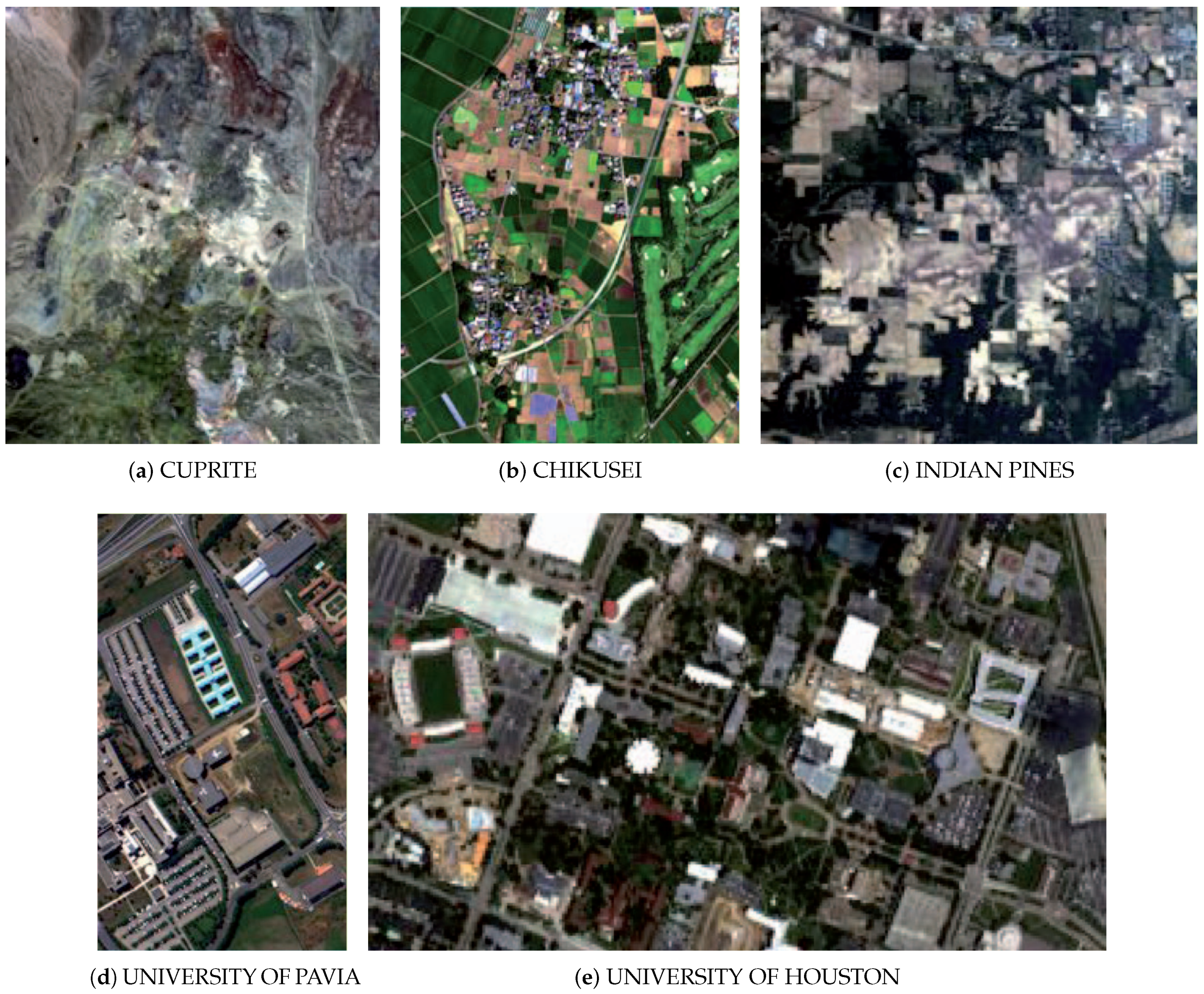
We used real-world images from standard HSI data sets, namely, the “Harvard” data set [36] and remote sensing image data sets. The remote sensing data we used were “CUPRITE”, “CHIKUSEI”, “INDIAN PINES”, “UNIVERSITY OF PAVIA”, and “UNIVERSITY OF HOUSTON”.

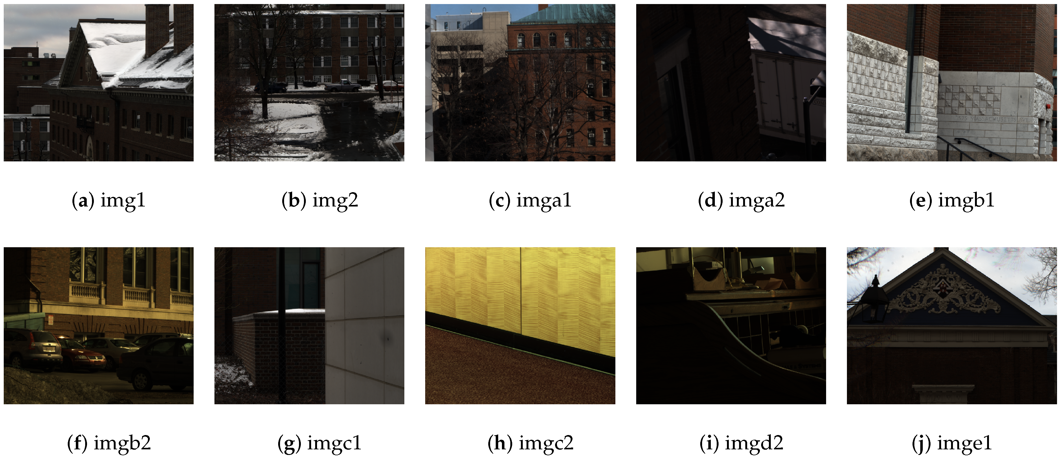
Images in the “Harvard” data set have a spatial resolution of $1392\times 1040$ and contain 31 spectral bands ranging from 420 nm to 720 nm. RGB color images from the “Harvard” data set are shown in Figure 1. In our experiments, the original images in the data sets served as ground truth. The observed low spatial resolution HSIs were downsampled by a factor of 8. Similarly, the conventional images (RGB color images) were downsampled in the spectral domain with a spectral response matrix R derived from a Nikon D700 digital camera (Nikon D700 Study http://www.maxmax.com/nikon_d700_study.htm).

CUPRITE is a data set which was captured in 1995 by the AVIRIS sensor over the Cuprite mining district in Nevada, shown in Figure 2a; CHIKUSEI was acquired in 2014 by a Headwall Hyperspectral Visible and Near-Infrared imaging sensor, shown in Figure 2b; INDIAN PINES is a data set captured in 1992 by the Airborne Visible/Infrared Imaging Spectrometer (AVIRIS) sensor over the Indian Pines test site in northwestern Indiana, shown in Figure 2c; UNIVERSITY OF PAVIA was taken by The Reflective Optics Spectrographic Imaging System (ROSIS)-3 optical airborne sensor over the University of Pavia in 2003, as shown in Figure 2d; and the UNIVERSITY OF HOUSTON data set was acquired by an ITRES Compact Airborne Spectrographic Imager (CASI)-1500 sensor over the University of Houston campus in 2013, as shown in Figure 2e. The main specifications of all the remote sensing data sets are summarized in

Table 1. Main specifications of the remote sensing data sets.

Data Sets	CUPRITE	CHIKUSEI	INDIAN PINES	PAVIA	HOUSTON
Spectral range ($\mathsf{\mu }\mathrm{m}$)	0.4–2.5	0.36–1.02	0.4–2.5	0.43–0.84	0.36–1.05
Total bands	224	128	224	115	144
Used bands	185	128	192	103	144
Total image size	512 × 614	2517 × 2335	512 × 614	610 × 340	349 × 1905
Used image size	420 × 360	540 × 320	360 × 360	560 × 320	320 × 540
Ground Sampling Distance	20	2.5	20	1.3	2.5
SNR	35	35	35	35	35

. It must be noted that we used cropped images with selected spectral bands, instead of the original images. Lines 4 and 6 in Table 1 show the number of selected bands and the size of the cropped image, which are essential parameters for the algorithms.

Six widely accepted quantitative metrics were used in this work to quantitatively measure the results. The basic idea of Structural Similarity (SSIM) [1] is to evaluate the similarity of two images through the following three aspects: luminance, contrast, and structure. It is formulated as follows:

$$\begin{array}{cc}\hfill SSIM& =f(l(S,\widehat{S}),c(S,\widehat{S}),s(S,\widehat{S}))\hfill \\ \hfill l(S,\widehat{S})=\frac{2{\mu }_S{\mu }_{\widehat{S}}+C_1}{{\mu }_S^2+{\mu }_{\widehat{S}}^2+C_1},c(S,\widehat{S})& =\frac{2{\sigma }_S{\sigma }_{\widehat{S}}+C_2}{{\sigma }_S^2+{\sigma }_{\widehat{S}}^2+C_2},s(S,\widehat{S})=\frac{{\sigma }_{S\widehat{S}}+C_3}{{\sigma }_S{\sigma }_{\widehat{S}}+C_3},\hfill \end{array}$$

(20)

where ${\mu }_S$ and ${\mu }_{\widehat{S}}$ represent the average values of the estimated image and ground truth, $\sigma$ is the standard deviation, and ${\sigma }_{S\widehat{S}}$ is the covariance of S and $\widehat{S}$. A SSIM value close to one indicates high image quality.

The root mean square error (RMSE) [1] measures the absolute error between the estimated image and the ground truth. A smaller RMSE value indicates better quality:

$$RMSE=\sqrt{\frac{\left|\right|\widehat{S}-S{\left|\right|}_F^2}{L{N}_c}},$$

(21)

where L is the number of bands and $N_c$ is the total number of pixels.

Peak signal-to-noise ratio (PSNR) [1] is used to measure the numerical similarity of spatial reconstruction between the result and the ground truth. It is defined as follows:

$$PSNR=10\times lo{g}_{10}\left(\frac{max{\left(S_i\right)}^2}{{∥S_i-{\widehat{S}}_i∥}_2^2/L}\right),$$

(22)

where $S_i$ and ${\widehat{S}}_i$ denote the pixel value of the ith spectral band separately in the reconstructed image and ground truth, respectively, and L is the total number of bands. The larger the PSNR value, the closer the spatial quality of the reconstructed image is to that of the reference image.

Spectral angle mapper (SAM) [1] is a metric which evaluates the spectral preservation quality, indicating the spectral similarity between the result and the ground truth. The SAM of the jth pixel is defined as the angle between the vectors of the estimated and the ground truth spectrum, as follows:

$$SAM=arccos\left(\frac{S_j^T{\widehat{S}}_j}{\left|\right|S_j{\left|\right|}_2\left|\right|{\widehat{S}}_j{\left|\right|}_2}\right).$$

(23)

A smaller SAM value indicates higher spectral quality.

The relative dimensionless global error in synthesis (ERGAS) [1] is a global statistical metric, which is defined as follows:

$$ERGAS=\frac{100}{d}\sqrt{\frac{1}{L}{\sum }_{i=1}^L\frac{MSE(S_i,{\widehat{S}}_i)}{mean{\left({\widehat{S}}_i\right)}^2}},$$

(24)

where $MSE(S_i,{\widehat{S}}_i)$ represents the mean square error, d is the downsampling scale factor, and $mean\left({\widehat{S}}_i\right)$ is the mean pixel value of ${\widehat{S}}_i$.

Hypercomplex quality assessment ($Q{2}^n$) [37] is another metric used to evaluate HSIs. $Q{2}^n$ has been improved based on the universal image quality index (UIQI), which has been widely used in many other related works. The UIQI is defined as:

$$\begin{array}{cc}\hfill & Q(x,y)=\frac{{\sigma }_{xy}}{{\sigma }_x{\sigma }_y}\frac{2\overline{x}\overline{y}}{{\overline{x}}^2{\overline{y}}^2}\frac{2{\sigma }_x{\sigma }_y}{{\sigma }_x^2+{\sigma }_y^2}\hfill \\ \hfill & \overline{x}=\frac{1}{L}\sum _{i=1}^L{x}_i,\overline{y}=\frac{1}{L}\sum _{i=1}^L{y}_i\hfill \\ \hfill {\sigma }_x=\sqrt{\frac{1}{L}\sum _{i=1}^L{(x_i-\overline{x})}^2},{\sigma }_y& =\sqrt{\frac{1}{L}\sum _{i=1}^L{(y_i-\overline{y})}^2},{\sigma }_{xy}=\frac{1}{L}\sum _{i=1}^L(x_i-\overline{x})(y_i-\overline{y}),\hfill \end{array}$$

(25)

where x and y are the band of ground truth and band of the reconstructed HSI. The three components of $Q(x,y)$ respectively represent the correlation, luminance distortion, and contrast distortion of the image. However, the UIQI was specifically designed for monochromatic images. $Q{2}^n$ overcomes this problem by modeling each pixel’s spectrum vector $x_j$ as a hypercomplex number, which is formulated as follows:

$$x_j=x_{j,0}+x_{j,1}{i}_1+x_{j,2}{i}_2\cdots +x_{j,2^n}{i}_{2^n-1}.$$

(26)

Thus, $Q{2}^n$ is a universal image metric, a larger value of which indicates higher quality of the image.

4.2. Experimental Setting

The basic procedure of the experiment was to first obtain the input images based on the ground truth image by simulation and then running various super-resolution algorithms to obtain high spatial resolution HSIs. Finally, the results were compared with the ground truth. The data sets provided an original HSI cube. There is no ground truth in the real world, so the literature typically uses the HSI in the data set as a reference. The input low spatial resolution HSIs and high spatial resolution conventional images were obtained by downsampling, based on these references.

The source code of all the related works for comparison are open-source. The code for FUSE is available at http://wei.perso.enseeiht.fr/publications.html; the code for BSR is available at http://openremotesensing.net/wp-content/uploads/2016/12/Supplementary.zip; the code for CSU is available at https://github.com/lanha/SupResPALM; the code for CMS is available at https://sites.google.com/site/leizhanghyperspectral/publications; and the code for LTTR is available at https://github.com/renweidian/LTTR.

We kept the default parameters for the related works. For the unmixing-based methods, the number of endmembers (P in Equation (1)) was set to 30, which was sufficient for all data sets. As for our spatial group sparsity regularization-based unmixing, the Lagrange multiplier regularization parameter $\mu$, the iteration number r, and the error tolerance $\epsilon$ were respectively set to $\mu ={10}^{-2}$, $r=1000$, and $\epsilon ={10}^{-6}$. Furthermore, the average width of the superpixels for SLIC was set to 10. The regularization parameter $\lambda$ plays an important role related to the trade-off between accuracy and sparsity, and was set to ${10}^{-2}$.

For images in the “Harvard” data set, all downsampling scale factors were set to 8. The conventional images had three spectral bands, which means that we estimated images with dimensions of $31\times 1392\times 1040$ from low spatial resolution hyperspectral images with dimensions of $31\times 174\times 130$ and conventional images with dimensions of $3\times 1392\times 1040$. For images in the remote sensing data sets, the downsampling scale factors and the numbers of conventional image bands were various, as shown in

Table 2. Parameters for the remote sensing data sets.

Data Sets	CUPRITE	CHIKUSEI	INDIAN PINES	PAVIA	HOUSTON
Bands of ground truth images	185	128	192	103	144
Bands of conventional images	16	8	16	4	4
Size of ground truth images	420 × 360	540 × 420	360 × 360	560 × 320	320 × 540
Size of hyperspectral images /Scale factor	84 × 72 /5	90 × 70 /6	90 × 90 /4	70 × 40 /8	64 × 108 /5

.

5. Results and Analysis

We present and analyze the performance of the proposed HSI super-resolution method in this section. Due to space limitations, not all results are presented. First, we give a visual result of our unmixing and super-resolution method. Then, examples of visual comparison results of images in the “Harvard” and “UNIVERSITY OF PAVIA” data sets are shown. Finally, we present the tables of objective image quality metrics of all the compared methods.

5.1. Hyperspectral Unmixing

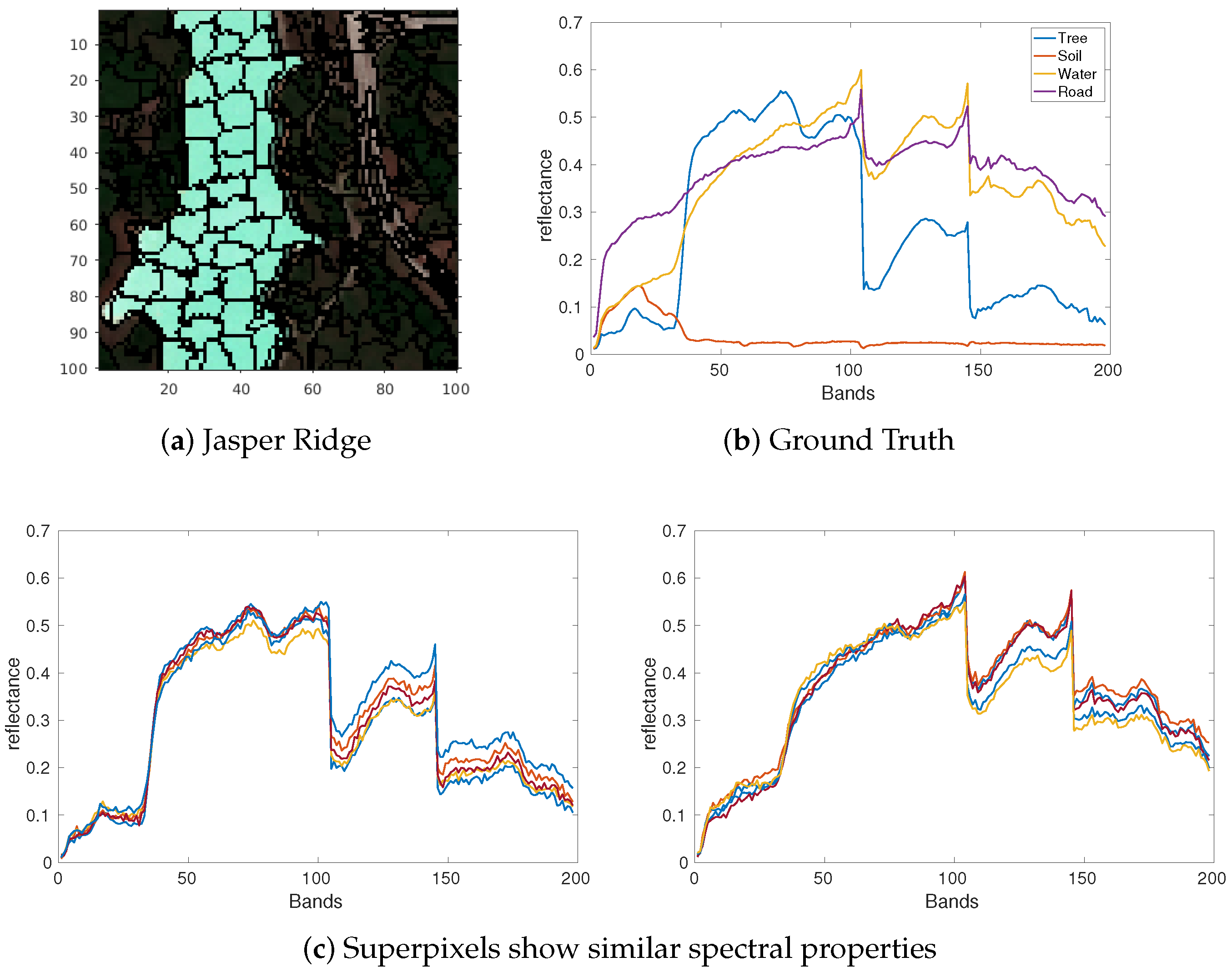
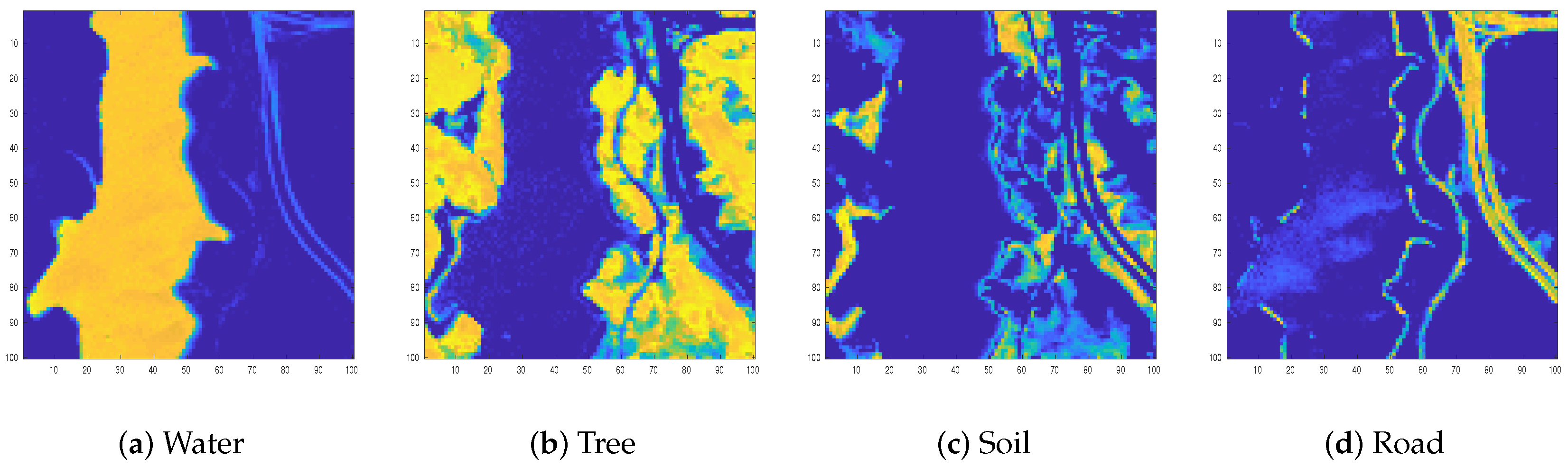
We selected a popular benchmark named “Jasper Ridge” as an example to qualitatively demonstrate the performance of the proposed hyperspectral unmixing method. It contained $100\times 100$ pixels with bands ranging from 380 nm to 2500 nm. The spectral resolution was up to 9.46 nm. Channels 1–3, 108–112, 154–166, and 220–224 were removed, in order to eliminate water absorption and atmospheric effects. Finally, 198 bands remained, and there were four latent endmembers in this data: “Water”, “Tree”, “Soil”, and “Road”. The SLIC superpixels of the benchmark “Jasper Ridge” are illustrated in Figure 3. The SLIC superpixels are shown in Figure 3a, whose shape and size are adaptive and related to the spectral similarity of the neighboring pixels. Figure 3b shows the ground truth spectral reflectances, while Figure 3c gives two examples that indicate pixels within a superpixel share similar spectral properties. The abundances were well estimated by the proposed method and were close to the ground truth. Figure 4 shows the estimated abundance.

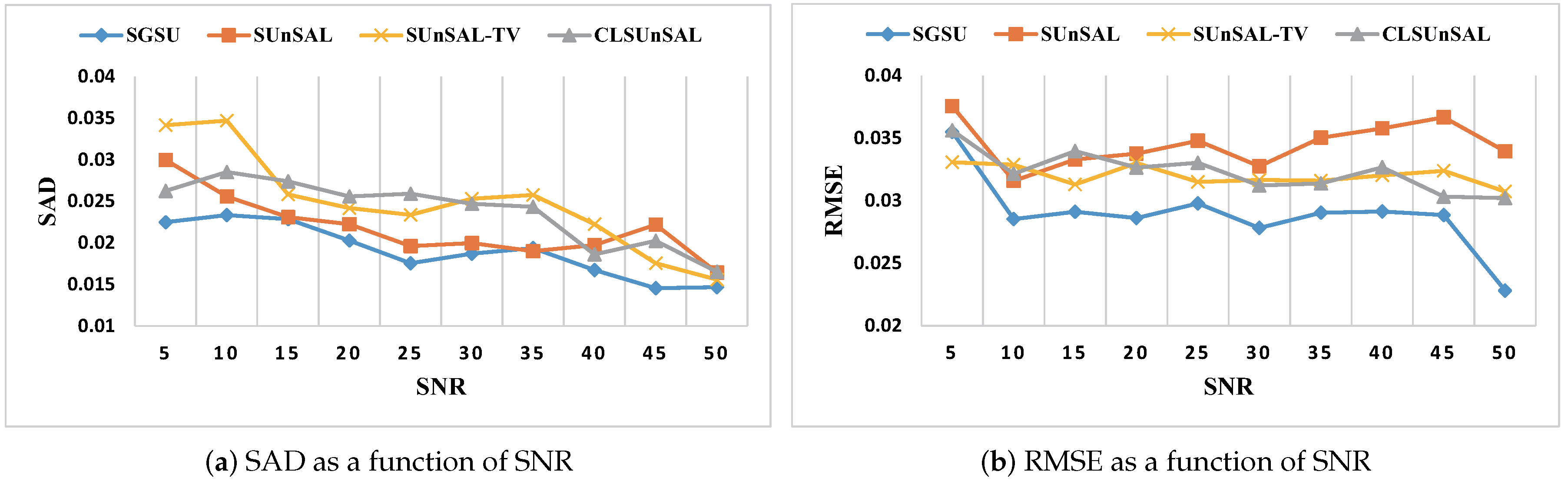
To verify the efficiency of the proposed Spatial Group Sparsity Regularization based unmixing (SGSU) algorithm, simulated experiments were performed. Synthetic HSIs with $100\times 100$ pixels contained six endmembers. The endmembers were randomly selected from the USGS library and randomly distributed. The proposed unmixing was compared to that of several typical sparse-based unmixing algorithms, such as SUnSAL [38], CLSUnSAL [39], and SUnSAL-TV [40]. The synthetic data were formed by spectra randomly selected from the digital spectral library of the United States Geological Survey (USGS), which is available at: https://www.usgs.gov/labs/spec-lab. We adopt two metrics to quantificationally evaluate the unmixing performance: the spectral angle difference (SAD) [41] and the root-mean-square error (RMSE) [41]. SAD and RMSE are typically used to evaluate the performance of hyperspectral unmixing. SAD is similar to SAM, as in Equation (20), but changes the input variable to endmembers. The input variable for RMSE is abundances. SAD was applied to evaluate the spectral angle between the estimated endmember and the ground truth endmember. RMSE is an evaluation metric for signal reconstruction, which represents the difference between the reconstructed signal and the original signal. Generally, smaller SAD and RMSE indicate better unmixing performance.

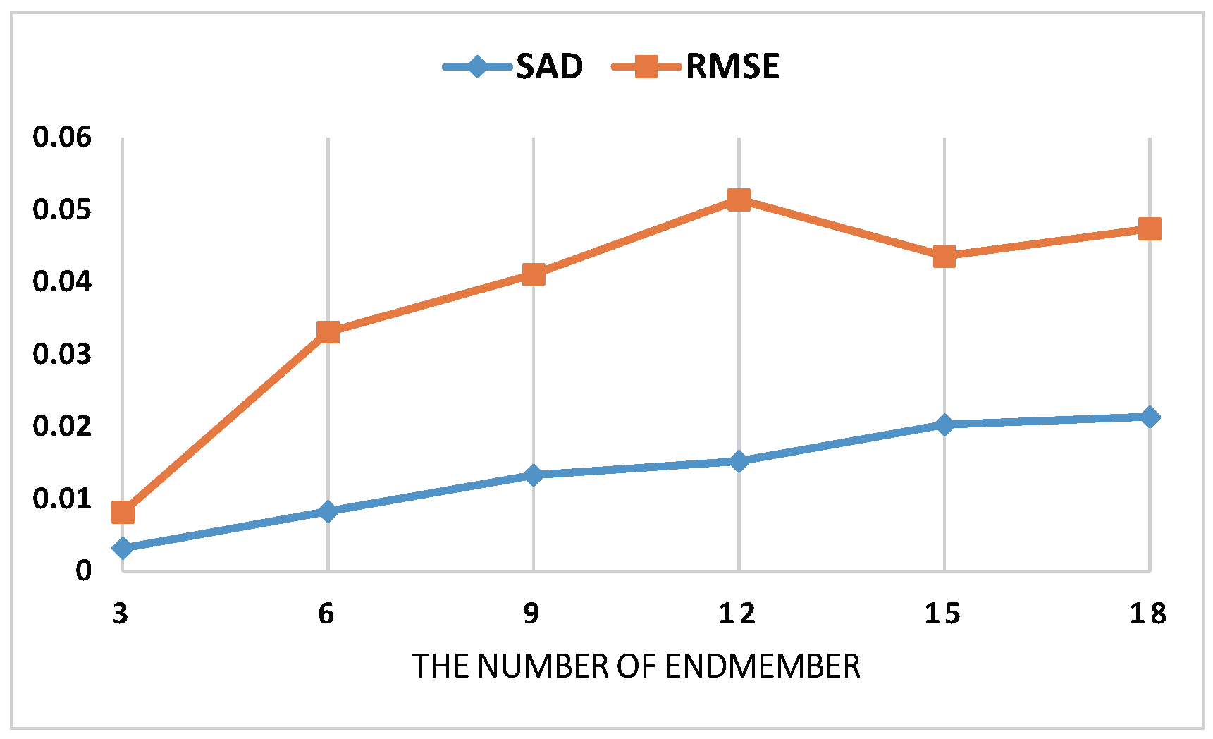
We conducted a experiment with the simulated data to analyze the sensitivity of the proposed unmixing method with regard to different endmember numbers. The number of endmembers was varied from 3 to 18 with a step length of 3. As Figure 5 shows that the values of SAD and RMSE increase as the number of endmembers increases, which means the difficulty of the unmixing increases as the number of endmembers increases. Noise and outliers also have significant impacts on hyperspectral unmixing. To study how the level of noise affects the unmixing performance and prove the superiority of the proposed unmixing method, we added Gaussian white noise with a signal-to-noise ratio (SNR) varying from 5 db to 50 db, and compared the proposed SGSU with some classical unmixing methods. Figure 6 shows the SAD and RMSE values as a function of the SNR of Gaussian white noise. We can see, from Figure 6a, that the SAD of all methods decreased with the increase of SNR, which indicates that noise had a bad effect on the hyperspectral unmixing. However, the proposed unmixing method obtained the best RMSE in most conditions; Figure 6b indicates that the proposed unmixing method performed better than other state-of-the-art methods.

5.2. Super-Resolution

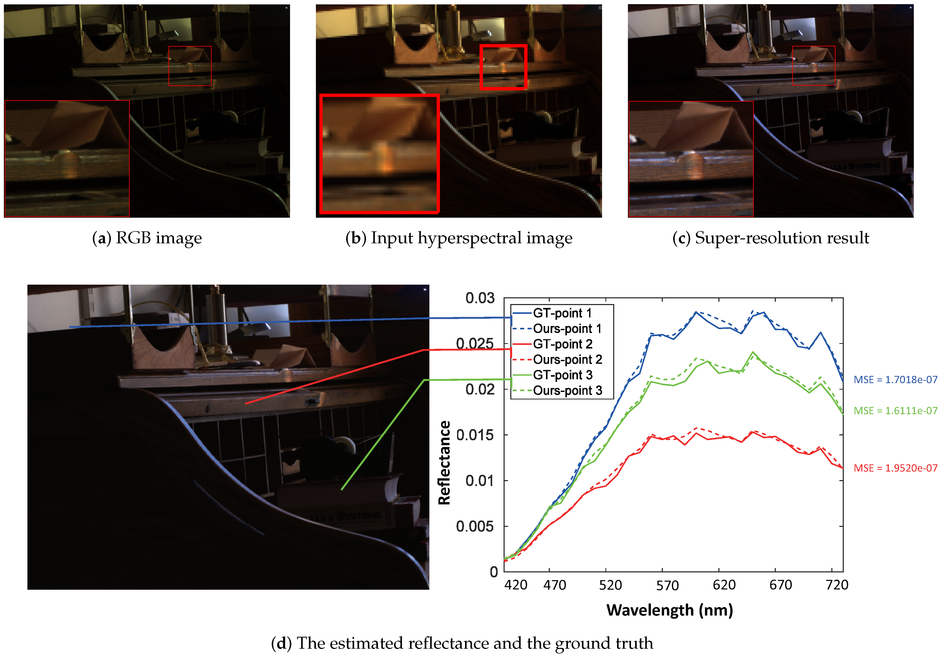
We show an example of the estimated super-resolution results in Figure 7. It was produced by using the proposed method on imgd2 of the “Harvard” data set, as shown in Figure 1i. Figure 7a–c show the input conventional (RGB) image, the low spatial resolution hyperspectral image, and the super-resolution result, respectively, where (b) and (c) are pseudo-color images with RGB bands set as (30,17,7).

A region of interest is magnified in each reconstructed image for better visual comparison. As can be seen from the magnified regions, Figure 7c shows that the reconstructed image had a good visual result and the same high spatial resolution as the RGB image. We also randomly selected three pixel points in the reconstructed image and the corresponding ground truth. The spectral responses of all the pixel points are shown in Figure 7d, where the solid lines are related to the ground truth and the dashed lines are related to the reconstructed image. The mean square error (MSE) values of the reconstructed spectral reflectance and the ground truth reflectance are presented in colors corresponding to the curves. The MSE values are very small, indicating that the reconstructed data were close to the ground truth data. In fact, in addition to the three example pixel-points, the spectral reflectances of other pixels were also reconstructed with high accuracy. Overall, these results show that our method has an efficient reconstruction performance in both spatial and spectral domains.

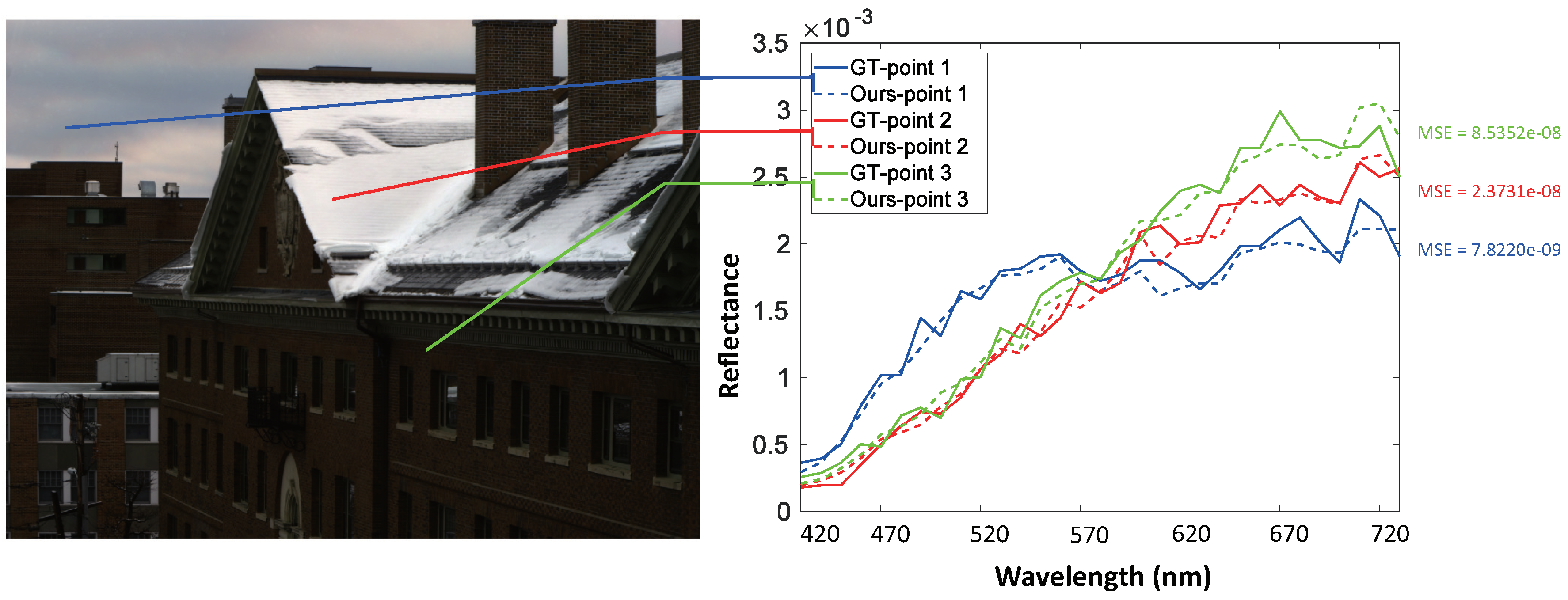
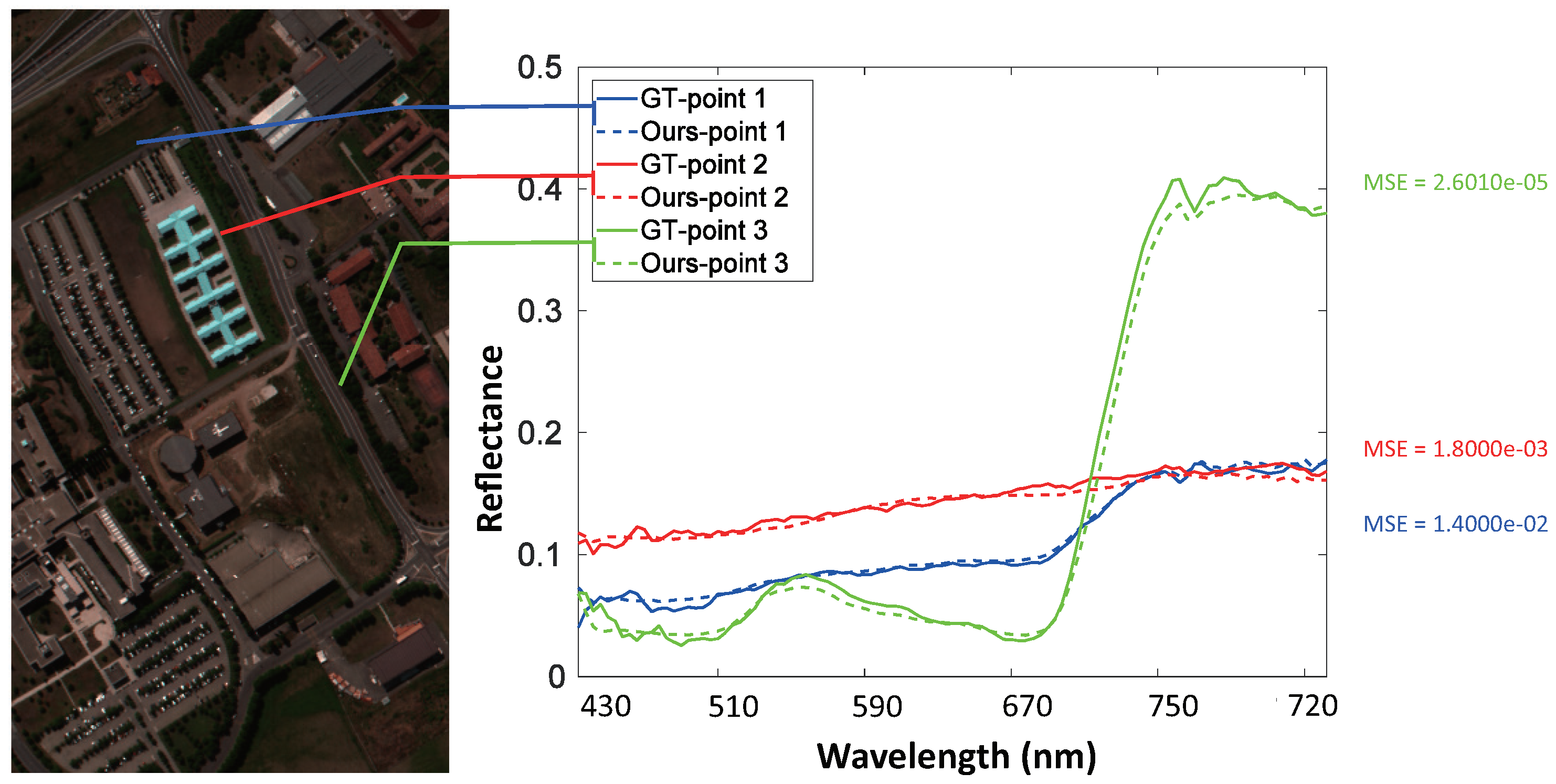
Figure 8 shows the estimated spectral reflectance of three randomly selected pixel points and their corresponding ground truths. The left image is the pseudo-color image of the super-resolution HSI of image1 in the “Harvard” data set. It has the same high spatial resolution as the input conventional image, which was presented in Figure 1a. The estimated reflectance curves visually match the ground truth well. The MSE of the estimated reflectances and the ground truth were very small, which indicates that the spectrum was efficiently reconstructed.

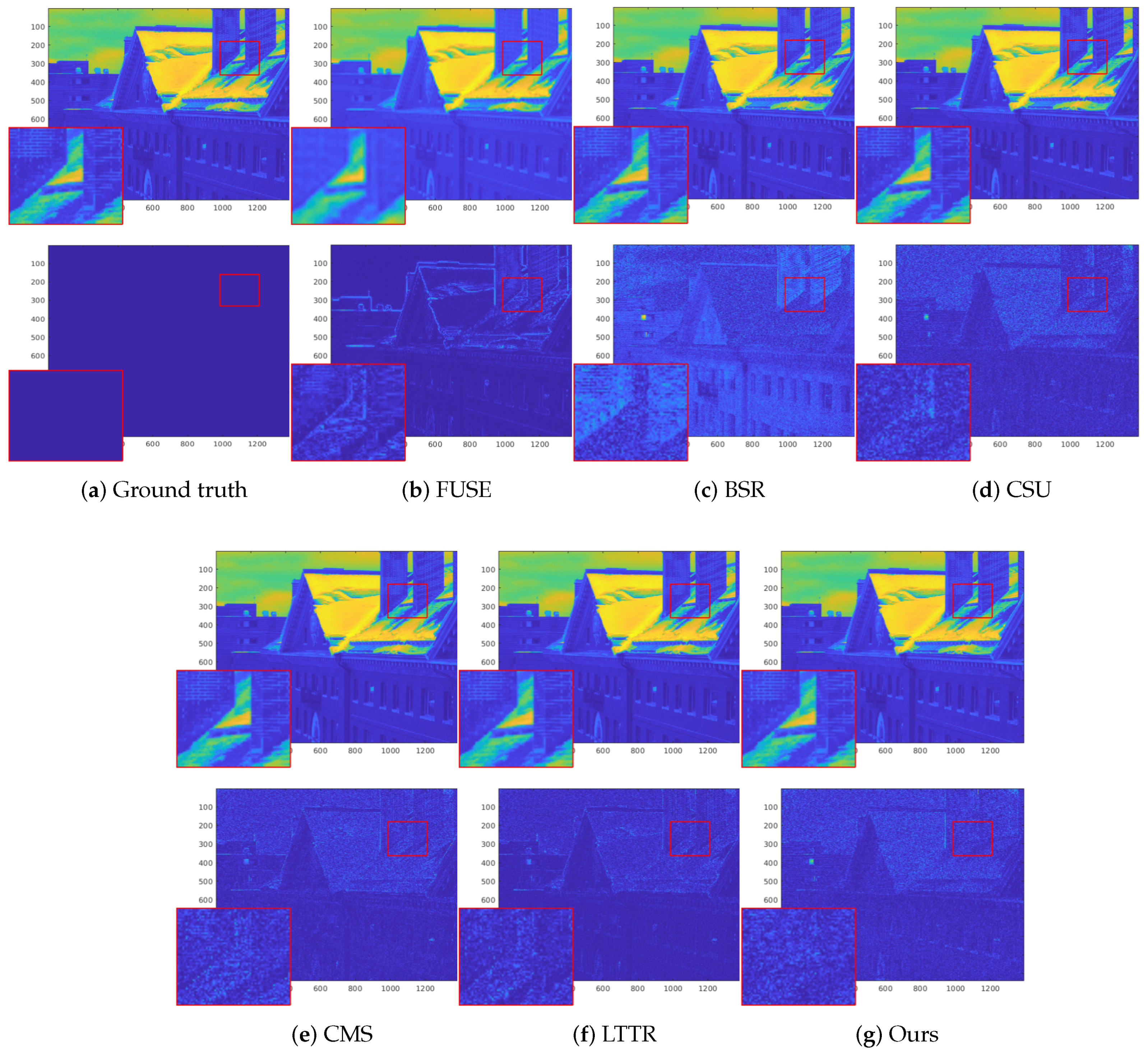
To compare our method with the other state-of-the-art methods, Figure 9 shows a visual comparison of all of the methods for image1 in the “Harvard” data set. For each sub-figure, the image on the top shows the super-resolution results of the corresponding methods in band 21 (620 nm) and image at the bottom is the error map, constructed by comparison with the ground truth. For ease of comparison, a region of interest is magnified in each reconstructed image. The smokestacks on the roof are highlighted by red squares. As we can see from Figure 9b,c, the results of FUSE were more blurry than the ground truth, and the results of BSR had the worst error map. Figure 9d–h show that CSU, CMS, and LTTR get close visual results to our method. However, if we check the region in the red square, the smokestack in the error map of sub-figure (g) is closer to zero than in (d), (e), and (f). This indicates that our method performed better in the reconstruction of detailed textures. Visual comparison by human eye is inevitably subjective and, therefore, quantitative objective evaluation is necessary.

For objective comparison, we carried out all methods to construct high resolution hyperspectral images from the input low spatial resolution hyperspectral images and conventional images. All quality metrics mentioned in Section 4.1 were applied to the resulting images and corresponding ground truth images. In particular, the images in the “Harvard” data set are all ground-based hyperspectral images, which have similar spatial and spectral properties. We give the mean and standard deviation for each quality metric in

Table 3. Average quantitative results of the compared methods on the Harvard data set.

Methods	FUSE	BSR	CSU	CMS	LTTR	Ours
SSIM	0.99902 ± 7.74 × 10${}^{-4}$	0.99943 ±6.9$\times {10}^{-4}$	0.99989 ±1.84× 10${}^{-4}$	0.99995 ±1.13$\times {10}^{-4}$	0.99991 ±1.23$\times {10}^{-4}$	0.99996 ±3.61$\times {10}^{-5}$
RMSE	0.48136 ±0.13070	0.28558 ±0.078466	0.23279 ±0.07063	0.22475 ±0.06109	0.24432 ±0.06109	0.21031 ±0.02689
PSNR	29.56316 ±4.23725	38.62009 ±5.45638	41.01761 ±5.27647	41.81752 ±5.81294	40.41452 ±5.52129	42.74880 ±2.89850
SAM	2.95474 ±0.793651	4.21175 ±1.31910	2.62583 ±0.86600	2.44085 ±0.75043	2.69322 ±0.76777	2.25826 ±0.58335
ERGAS	2.78576 ±1.21321	1.38858 ±0.69591	1.08028 ±0.71299	0.91274 ±0.47246	1.02112 ±0.49095	0.86787 ±0.52625
$Q{2}^n$	0.53836 ±0.10412	0.75601 ±0.09046	0.81238 ±0.06793	0.80453 ±0.06697	0.78496 ±0.07007	0.82477 ±0.05305
Time (s)	10.66	8157.12	1358.69	1388.09	1631.74	2369.83

. The best results are shown in bold.

Note that Table 3 gives an evaluation of the overall image quality, while Figure 9 shows a visual comparison in a single band. Hence, it is reasonable that the subjective evaluation of Figure 9 might be inconsistent with some of the metrics in Table 3. This inconsistency does not affect the conclusions of the quantitative quality evaluation.

It can be seen, from the numerical results in Table 3, that the proposed method had superior performance to the compared methods, in terms of all quality metrics. All of the methods performed well in terms of SSIM. The superiority in SSIM values demonstrates that the spatial structures of the estimated hyperspectral images were well-recovered by the proposed method. Our method achieved a significantly lower average RMSE than all other compared methods. It reduced the error by about 6.4%, compared to the best baseline and improved at least 56.3% against all others. The superiority in RMSE indicates that our estimated image had the closest pixel values to the ground truth in all spectral bands. The average PSNR of the proposed method was 0.93–11.01 db (2.22% to 37.25%) larger than that of the other methods. This indicates that the super-resolution results obtained by the proposed method were closer to the ground truth, in terms of spatial numerical similarity. SSIM, RMSE, and PSNR all mainly evaluate performance in terms of spatial information. This improvement is a result of using the SLIC superpixel algorithm in our method. Spatially adjacent pixels are clustered, in order to take advantage of preserving structures or features with similar structures. SAM evaluates the quality of spectral reconstruction. It can be seen that the average SAM value of the proposed method was lower than that of the compared methods. Our average SAM value was reduced by 46.38% to 7.48%, compared to the other baselines. The superiority in spectral similarity of the proposed method comes from the sparsity priors by coupling a spatial group sparsity regularizer with sparse unmixing. ERGAS and $Q{2}^n$ are global quality metrics, which not only evaluate the spatial structure but also the spectral similarity. As shown in Table 3, the ERGAS produced by our method was 4.92% less than the second-best performed baseline and 68.85% less than the worst-performing baseline.

It should be noted that, in Table 3, the number before the symbol “±” is the average value and the number after the symbol “±” is the standard deviation. The standard deviation indicates how the quality metric values differ from the average value. We can observe that our method obtained the best average values and the smallest standard deviations (except for ERGAS), which means our method not only performed better but was also more stable than the other compared methods.

Similarly, in Figure 10, the estimated spectral responses and the ground truth for the “UNIVERSITY OF PAVIA” data set are shown. The pseudo-color image of the super-resolution HSI is presented on the left side. It was visually well-reconstructed, compared to the input conventional image, as shown in Figure 2d. Our method also obtained a satisfactory result, in terms of spectrum reconstruction. As shown in the reflectance curves on the right side, the spectra of three randomly selected pixel points were well-reconstructed.

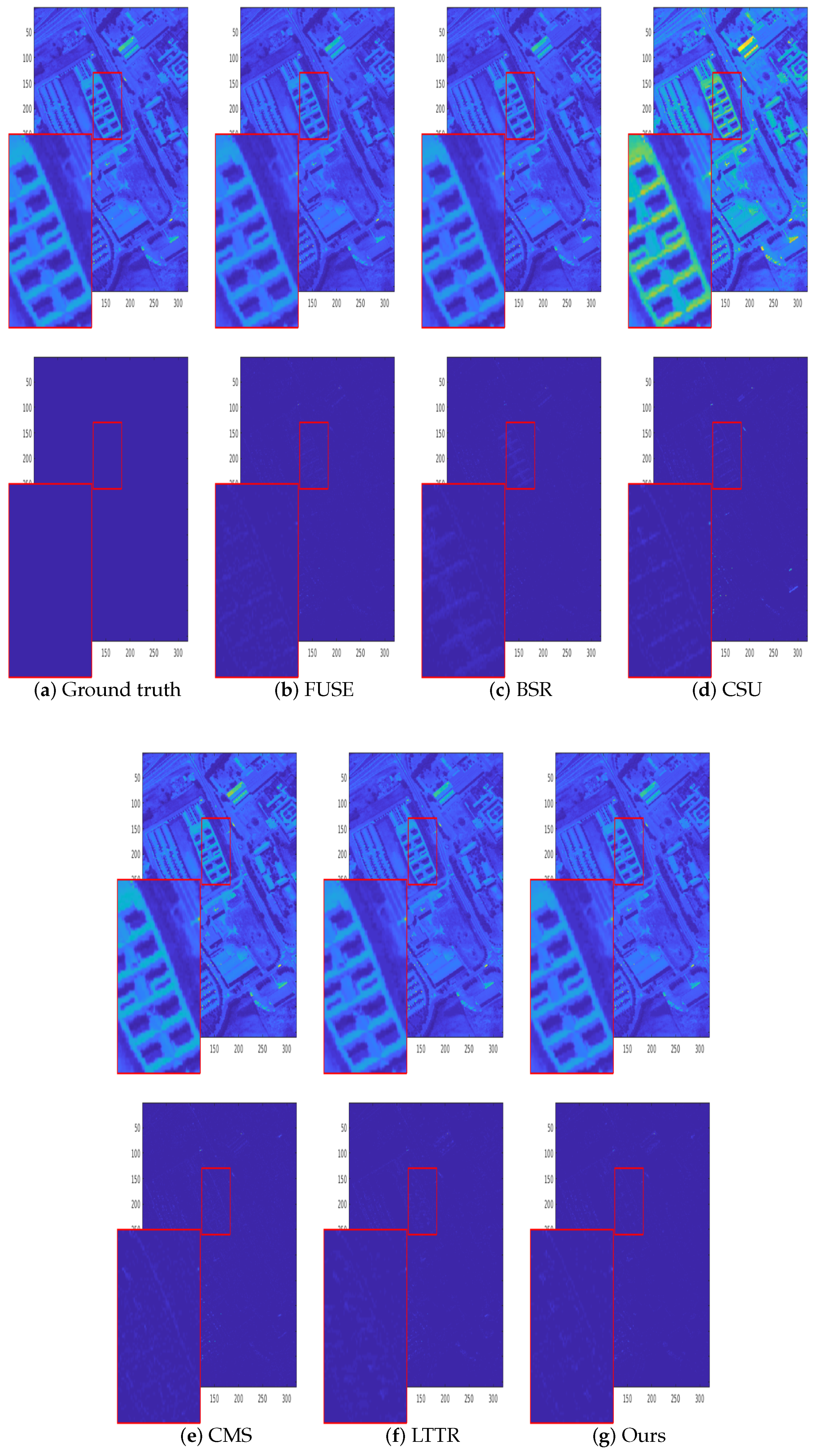
As an example of visual results for the remote sensing data sets considered, Figure 11 shows a visual comparison of the results of all the considered methods for the “UNIVERSITY OF PAVIA” data set. The CSU results show an obvious difference from the ground truth. A careful check of the building in the red square reveals that the error maps of FUSE, BSR, and CSU show an obvious shadow of the building. The error maps of CMS, LTTR, and Ours were closer to the ground truth. The bottom three error maps were very close to each other, but we can still see that our method achieved a smaller reconstruction error, indicating that the proposed method could reconstruct detailed spatial structures more accurately. Considering the visual deviation of the human eye, a quantitative comparison for remote sensing data sets is presented in the following discussion.

Similar to the “Harvard” data set,

Table 4. Quantitative results of the compared methods on the Remote sensing data sets.

	Methods	FUSE	BSR	CSU	CMS	LTTR	Ours
CUPRITE	SSIM	0.83747	0.98963	0.99192	0.97348	0.95545	0.99238
	RMSE	4.9375	1.15290	1.0562	2.08420	2.15130	0.98903
	PSNR	31.6723	41.1775	41.8221	37.0663	40.8065	42.6838
	SAM	3.635	0.76047	0.65195	0.88845	0.93718	0.62051
	ERGAS	1.2788	0.3173	0.29971	0.54418	0.55328	0.26375
	$Q{2}^n$	0.80201	0.97817	0.97233	0.89626	0.97452	0.97993
	Time (s)	1.29	2022.60	111.01	206.09	340.67	131.65
CHIKUSEI	SSIM	0.99651	0.99575	0.99603	0.98038	0.99215	0.99706
	RMSE	1.1972	1.2076	1.1823	2.9822	1.7675	1.0371
	PSNR	45.4159	43.9835	42.4042	38.7097	42.6187	44.4753
	SAM	1.4699	1.5546	1.3871	2.2058	2.0718	1.2426
	ERGAS	1.6222	1.8631	1.7196	1.7487	1.6666	1.6081
	$Q{2}^n$	0.91975	0.94963	0.91864	0.86428	0.87594	0.92592
	Time (s)	2.91	2235.74	233.58	203.61	720.26	265.67
INDIAN PINES	SSIM	0.90796	0.98916	0.98807	0.97736	0.97826	0.99075
	RMSE	9.5287	1.3632	1.5157	2.2509	1.6519	1.3892
	PSNR	35.5488	40.4208	41.3034	40.1867	41.0773	42.9987
	SAM	6.4675	0.79846	0.88154	0.96104	0.83385	0.82111
	ERGAS	1.7171	0.4197	0.41053	0.55839	0.58602	0.33396
	$Q{2}^n$	0.38834	0.76825	0.70134	0.81233	0.88700	0.71257
	Time (s)	2.80	1924.67	157.41	280.83	570.40	173.08
UNIVERSITY OF PAVIA	SSIM	0.9805	0.98122	0.98029	0.94498	0.93797	0.98206
	RMSE	2.0836	2.1192	2.3904	4.3442	4.5258	2.0834
	PSNR	41.6695	41.6288	39.5331	35.8998	35.9253	41.0519
	SAM	2.8931	3.0125	2.7325	4.3366	5.1832	2.6367
	ERGAS	0.83523	0.86948	0.97139	1.5170	1.8383	0.8492
	$Q{2}^n$	0.88702	0.87856	0.80358	0.62222	0.59185	0.84299
	Time (s)	1.98	1648.0	175.0	210.96	424.48	203.73
UNIVERSITY OF HOUSTON	SSIM	0.95808	0.95452	0.96435	0.76379	0.64306	0.96456
	RMSE	7.6814	8.5580	7.3756	20.9834	24.4054	7.3900
	PSNR	32.155	31.574	32.7052	23.8961	28.877	32.7105
	SAM	2.2091	2.2500	2.0754	4.7053	6.2191	2.0917
	ERGAS	3.4876	3.9151	3.255	8.2063	5.1517	3.2605
	$Q{2}^n$	0.90252	0.88463	0.90889	0.69074	0.65189	0.91488
	Time (s)	1.47	1904.26	145.68	93.79	638.94	114.72

shows the results for all of the remote sensing data sets. The best values are highlighted in bold. In addition, if our method did not achieve the best result in a certain metric, but the second-best, it is highlighted and underlined.

All quality metrics of the proposed method on the “CUPRITE” data set outperformed the other methods. For the “CHIKUSEI” data set, the values of PSNR and $Q{2}^n$ for the proposed method were the second-best in all methods, while SSIM, RMSE, SAM, and ERGAS were all the best. For the “INDIAN PINES” data set, our method obtained the best SSIM, PSNR, SAM, and ERGAS, and the second-best RMSE. For the “UNIVERSITY OF PAVIA” data set, our method obtained the best SSIM, RMSE, and SAM, and the second-best $Q{2}^n$. For the “UNIVERSITY OF HOUSTON” data set, all quality metrics were superior, except for RMSE (which was the second-best).

5.3. Impact on Classification

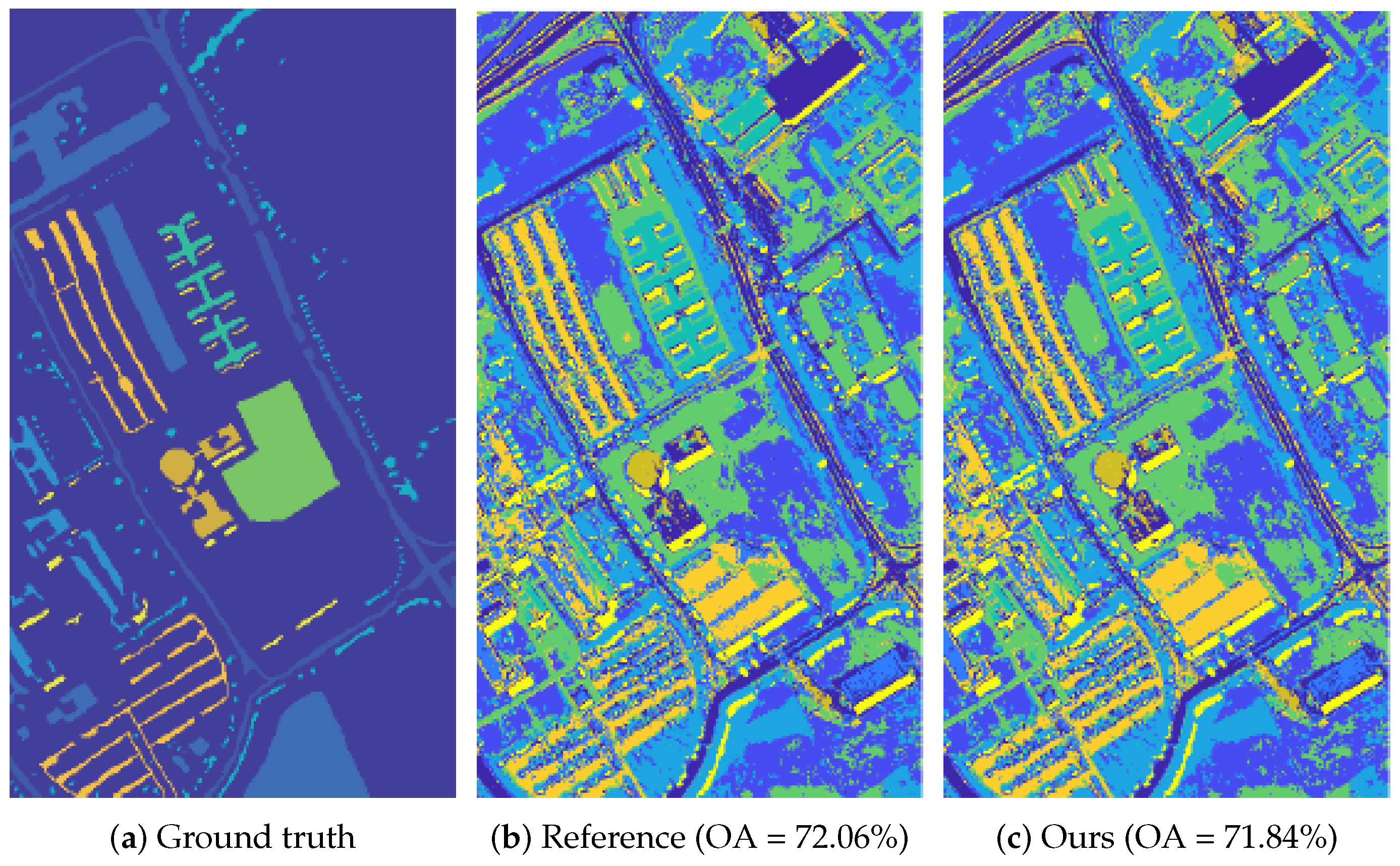
HSI classification is one of the most relevant topics in HSI processing. The quality of the fused images can be indirectly validated by pixel-wise classification. The classification performance was quantitatively validated using the overall accuracy (OA). The classification method we used is based on the K-Nearest Neighbors (KNN) classifier [42]. As the absolute OA value for classification is not mainly concerned in this paper, we set the parameter k as 5 and the ratio of training data as 0.1 for lower processing time. This led to not very high OA results, but this did not affect the verification of our super-resolution method. The “UNIVERSITY OF PAVIA” data set has also been widely used in HSI classification, due to the availability of ground truth data. The classification results of our method are shown in Figure 12, where sub-figure (a) shows the ground truth classification map, sub-figure (b) shows the reference classification map (which is the result of the original high spatial resolution HSI), and sub-figure (c) shows the classification map of our super-resolution HSI.

Table 5. Classification result comparison for the UNIVERSITY OF PAVIA data set.

Methods	Reference	FUSE	BSR	CSU	CMS	LTTR	Ours
OA	72.06%	70.39%	70.07%	71.43%	69.84%	70.82%	71.84%

shows the quantitative numerical results of all methods for comparison. From the results, we can make the observation that our super-resoultion HSI can obtain a closer OA to the original HSI than any of the other considered methods.

5.4. Computational Cost

To evaluate the computational cost of the proposed work, we report the runtime for all methods in Table 3 and Table 4, which were obtained by reconstructing the HSIs from the corresponding data sets. BSR was the most time-consuming method, as it needs to learn a dictionary for sparse coding. FUSE is a simple fusion strategy, making it the fastest method; however, it had poor super-resolution performance. Compared with the rest of the methods, the time consumed by our method was moderate and acceptable. For the “Harvard” data set, our method did not have a superior performance in run-time. This was due to the super-pixel procedure in our method, the run-time of which is mainly influenced by image size. For all remote sensing data sets, the run-time of our method was superior to that of LTTR but worse than that of CSU. Considering both HSI super-resolution and computational cost, the method proposed in this paper can be considered effective.

6. Conclusions

This paper proposed an HSI super-resolution method based on spatial group sparsity regularization unmixing. It can construct a high spatial and spectral resolution HSI from a low spatial resolution HSI and a high spatial resolution conventional image by solving the spectral unmixing problem for both input images. The unmixing-based super-resolution of the HSI helps to alleviate the constraints derived from the imaging process. Under the linear mixing model, the proposed unmixing method integrates the advantages of both spatial group sparsity and the ${\ell }_{2,1}$ norm to produce a more accurate and robust unmixing estimation. The SLIC superpixel algorithm is used to transform the original hyperspectral data, making full use of the spatial information and sparse priors. The SLIC superpixel algorithm is used to transform the original HSI into spatial groups. Then, the distribution of the endmembers is estimated based on the spatial and sparsity priors. The proposed method takes advantage of this distribution estimate as a regularizer for sparse unmixing and solves for the abundances using the ADMM algorithm. The spatial group sparsity regularization unmixing makes full use of the spatial structure and the spectra of the images. In simulations on public data sets—a ground-based data set “Harvard” and five satellite remote sensing data sets—the proposed method showed superior performance, when compared to state-of-the-art methods.

References

- Yokoya, N.; Grohnfeldt, C.; Chanussot, J. Hyperspectral and multispectral data fusion: A comparative review of the recent literature. IEEE Geosci. Remote Sens. Mag. 2017, 5, 29–56. [Google Scholar] [CrossRef]
- Sankararaman, S.P. Tissue Characterization by Deep Learning in Medical Hyperspectral Images; Delft University of Technology: Delft, The Netherland, 2019. [Google Scholar]
- Liu, Y.; Tao, Z.; Zhang, J.; Hao, H.; Peng, Y.; Hou, J.; Jiang, T. Deep-Learning-Based Active Hyperspectral Imaging Classification Method Illuminated by the Supercontinuum Laser. Appl. Sci. 2020, 10, 3088. [Google Scholar] [CrossRef]
- Liu, Y.; Su, M.; Liu, L.; Li, C.; Peng, Y.; Hou, J.; Jiang, T. Deep residual prototype learning network for hyperspectral image classification. In Proceedings of the Second Target Recognition and Artificial Intelligence Summit Forum, Tirana, Albania, 11–13 December 2020; Volume 11427, p. 1142705. [Google Scholar]
- Uzkent, B.; Rangnekar, A.; Hoffman, M. Aerial vehicle tracking by adaptive fusion of hyperspectral likelihood maps. In Proceedings of the IEEE Conference on Computer Vision and Pattern Recognition Workshops, Honolulu, HI, USA, 21–26 July 2017; pp. 39–48. [Google Scholar]
- Bitar, A.W.; Cheong, L.F.; Ovarlez, J.P. Sparse and low-rank matrix decomposition for automatic target detection in hyperspectral imagery. IEEE Trans. Geosci. Remote Sens. 2019, 57, 5239–5251. [Google Scholar] [CrossRef] [Green Version]
- Akgun, T.; Altunbasak, Y.; Mersereau, R.M. Super-resolution reconstruction of hyperspectral images. IEEE Trans. Image Process. 2005, 14, 1860–1875. [Google Scholar] [CrossRef] [PubMed]
- Li, C.; Sun, T.; Kelly, K.F.; Zhang, Y. A compressive sensing and unmixing scheme for hyperspectral data processing. IEEE Trans. Image Process. 2011, 21, 1200–1210. [Google Scholar]
- Gomez, R.B.; Jazaeri, A.; Kafatos, M. Wavelet-based hyperspectral and multispectral image fusion. In Proceedings of the Geo-Spatial Image and Data Exploitation II, Orlando, FL, USA, 1 June 2001; Volume 4383, pp. 36–42. [Google Scholar]
- Zhang, Y.; He, M. Multi-spectral and hyperspectral image fusion using 3D wavelet transform. J. Electron. (China) 2007, 24, 218–224. [Google Scholar] [CrossRef]
- Chen, Z.; Pu, H.; Wang, B.; Jiang, G.M. Fusion of hyperspectral and multispectral images: A novel framework based on generalization of pan-sharpening methods. IEEE Geosci. Remote Sens. Lett. 2014, 11, 1418–1422. [Google Scholar] [CrossRef]
- Berné, O.; Helens, A.; Pilleri, P.; Joblin, C. Non-negative matrix factorization pansharpening of hyperspectral data: An application to mid-infrared astronomy. In Proceedings of the IEEE 2010 2nd Workshop on Hyperspectral Image and Signal Processing: Evolution in Remote Sensing, Amsterdam, The Netherlands, 30 September–2 October 2010; pp. 1–4. [Google Scholar]
- Yokoya, N.; Yairi, T.; Iwasaki, A. Coupled nonnegative matrix factorization unmixing for hyperspectral and multispectral data fusion. IEEE Trans. Geosci. Remote Sens. 2011, 50, 528–537. [Google Scholar] [CrossRef]
- Dian, R.; Fang, L.; Li, S. Hyperspectral image super-resolution via non-local sparse tensor factorization. In Proceedings of the IEEE Conference on Computer Vision and Pattern Recognition, Honolulu, HI, USA, 21–26 July 2017; pp. 5344–5353. [Google Scholar]
- Li, S.; Dian, R.; Fang, L.; Bioucas-Dias, J.M. Fusing hyperspectral and multispectral images via coupled sparse tensor factorization. IEEE Trans. Image Process. 2018, 27, 4118–4130. [Google Scholar] [CrossRef]
- Qu, Y.; Qi, H.; Kwan, C. Unsupervised sparse dirichlet-net for hyperspectral image super-resolution. In Proceedings of the IEEE Conference on Computer Vision and Pattern Recognition, Salt Lake City, UT, USA, 18–22 June 2018; pp. 2511–2520. [Google Scholar]
- Xie, Q.; Zhou, M.; Zhao, Q.; Meng, D.; Zuo, W.; Xu, Z. Multispectral and hyperspectral image fusion by MS/HS fusion net. In Proceedings of the IEEE Conference on Computer Vision and Pattern Recognition, Alexandria, Egypt, 10 January 2019; pp. 1585–1594. [Google Scholar]
- Dobigeon, N.; Tourneret, J.Y.; Richard, C.; Bermudez, J.C.M.; McLaughlin, S.; Hero, A.O. Nonlinear unmixing of hyperspectral images: Models and algorithms. IEEE Signal Process. Mag. 2013, 31, 82–94. [Google Scholar] [CrossRef] [Green Version]
- Imbiriba, T.; Borsoi, R.A.; Bermudez, J.C.M. Generalized linear mixing model accounting for endmember variability. In Proceedings of the 2018 IEEE International Conference on Acoustics, Speech and Signal Processing (ICASSP), Calgary, AB, Canada, 15–20 April 2018; pp. 1862–1866. [Google Scholar]
- Huang, B.; Song, H.; Cui, H.; Peng, J.; Xu, Z. Spatial and spectral image fusion using sparse matrix factorization. IEEE Trans. Geosci. Remote Sens. 2013, 52, 1693–1704. [Google Scholar] [CrossRef]
- Selva, M.; Aiazzi, B.; Butera, F.; Chiarantini, L.; Baronti, S. Hyper-sharpening: A first approach on SIM-GA data. IEEE J. Sel. Top. Appl. Earth Obs. Remote Sens. 2015, 8, 3008–3024. [Google Scholar] [CrossRef]
- Akhtar, N.; Shafait, F.; Mian, A. Bayesian sparse representation for hyperspectral image super resolution. In Proceedings of the IEEE Conference on Computer Vision and Pattern Recognition, Boston, MA, USA, 7–12 June 2015; pp. 3631–3640. [Google Scholar]
- Lanaras, C.; Baltsavias, E.; Schindler, K. Hyperspectral super-resolution by coupled spectral unmixing. In Proceedings of the IEEE International Conference on Computer Vision, Santiago, Chile, 7–13 December 2015; pp. 3586–3594. [Google Scholar]
- Akhtar, N.; Shafait, F.; Mian, A. Sparse spatio-spectral representation for hyperspectral image super-resolution. In Proceedings of the European Conference on Computer Vision, Zurich, Switzerland, 6–12 September 2014; Springer: Berlin/Heidelberg, Germany, 2014; pp. 63–78. [Google Scholar]
- Wei, Q.; Bioucas-Dias, J.; Dobigeon, N.; Tourneret, J.Y.; Chen, M.; Godsill, S. Multiband image fusion based on spectral unmixing. IEEE Trans. Geosci. Remote Sens. 2016, 54, 7236–7249. [Google Scholar] [CrossRef] [Green Version]
- Zhang, L.; Wei, W.; Bai, C.; Gao, Y.; Zhang, Y. Exploiting clustering manifold structure for hyperspectral imagery super-resolution. IEEE Trans. Image Process. 2018, 27, 5969–5982. [Google Scholar] [CrossRef] [PubMed]
- Yi, C.; Zhao, Y.Q.; Chan, J.C.W.; Kong, S.G. Joint Spatial-spectral Resolution Enhancement of Multispectral Images with Spectral Matrix Factorization and Spatial Sparsity Constraints. Remote Sens. 2020, 12, 993. [Google Scholar] [CrossRef] [Green Version]
- Saragadam, V.; Sankaranarayanan, A.C. KRISM—Krylov subspace-based optical computing of hyperspectral images. ACM Trans. Graph. (TOG) 2019, 38, 1–14. [Google Scholar] [CrossRef] [Green Version]
- Zhang, K.; Wang, M.; Yang, S.; Jiao, L. Spatial–spectral-graph-regularized low-rank tensor decomposition for multispectral and hyperspectral image fusion. IEEE J. Sel. Top. Appl. Earth Obs. Remote Sens. 2018, 11, 1030–1040. [Google Scholar] [CrossRef]
- Bengua, J.A.; Phien, H.N.; Tuan, H.D.; Do, M.N. Efficient tensor completion for color image and video recovery: Low-rank tensor train. IEEE Trans. Image Process. 2017, 26, 2466–2479. [Google Scholar] [CrossRef] [Green Version]
- Dian, R.; Li, S.; Fang, L. Learning a low tensor-train rank representation for hyperspectral image super-resolution. IEEE Trans. Neural Netw. Learn. Syst. 2019, 30, 2672–2683. [Google Scholar] [CrossRef]
- Zhang, T.; Fu, Y.; Wang, L.; Huang, H. Hyperspectral Image Reconstruction Using Deep External and Internal Learning. In Proceedings of the IEEE International Conference on Computer Vision, Tokyo, Japan, 12–15 April 2019; pp. 8559–8568. [Google Scholar]
- Ma, Y.; Li, C.; Mei, X.; Liu, C.; Ma, J. Robust Sparse Hyperspectral Unmixing With ell_{2, 1} Norm. IEEE Trans. Geosci. Remote Sens. 2016, 55, 1227–1239. [Google Scholar] [CrossRef]
- Achanta, R.; Shaji, A.; Smith, K.; Lucchi, A.; Fua, P.; Süsstrunk, S. SLIC superpixels compared to state-of-the-art superpixel methods. IEEE Trans. Pattern Anal. Mach. Intell. 2012, 34, 2274–2282. [Google Scholar] [CrossRef] [PubMed] [Green Version]
- Wei, Q.; Dobigeon, N.; Tourneret, J.Y. Fast fusion of multi-band images based on solving a Sylvester equation. IEEE Trans. Image Process. 2015, 24, 4109–4121. [Google Scholar] [CrossRef] [PubMed] [Green Version]
- Chakrabarti, A.; Zickler, T. Statistics of real-world hyperspectral images. In Proceedings of the IEEE CVPR 2011, Seattle, WA, USA, 21–23 June 2011; pp. 193–200. [Google Scholar]
- Garzelli, A.; Nencini, F. Hypercomplex quality assessment of multi/hyperspectral images. IEEE Geosci. Remote Sens. Lett. 2009, 6, 662–665. [Google Scholar] [CrossRef]
- Bioucas-Dias, J.M.; Figueiredo, M.A. Alternating direction algorithms for constrained sparse regression: Application to hyperspectral unmixing. In Proceedings of the IEEE 2010 2nd Workshop on Hyperspectral Image and Signal Processing: Evolution in Remote Sensing, Reykjavik, Iceland, 14–16 June 2010; pp. 1–4. [Google Scholar]
- Iordache, M.D.; Bioucas-Dias, J.M.; Plaza, A. Collaborative sparse regression for hyperspectral unmixing. IEEE Trans. Geosci. Remote Sens. 2013, 52, 341–354. [Google Scholar] [CrossRef] [Green Version]
- Iordache, M.D.; Bioucas-Dias, J.M.; Plaza, A. Total variation regulatization in sparse hyperspectral unmixing. In Proceedings of the IEEE 2011 3rd Workshop on Hyperspectral Image and Signal Processing: Evolution in Remote Sensing (WHISPERS), Cambridge, MA, USA, 6–9 June 2011; pp. 1–4. [Google Scholar]
- Wang, X.; Zhong, Y.; Zhang, L.; Xu, Y. Spatial group sparsity regularized nonnegative matrix factorization for hyperspectral unmixing. IEEE Trans. Geosci. Remote. Sens. 2017, 55, 6287–6304. [Google Scholar] [CrossRef]
- Ma, L.; Crawford, M.M.; Tian, J. Local manifold learning-based k-nearest-neighbor for hyperspectral image classification. IEEE Trans. Geosci. Remote Sens. 2010, 48, 4099–4109. [Google Scholar] [CrossRef]
Figure 1.
Images from the Harvard data set.
Figure 2.
Remote sensing images.
Figure 3.
Illustration of SLIC superpixels.
Figure 4.
Estimated abundances.
Figure 5.
SAD and RMSE with a different number of endmembers.
Figure 6.
SAD and RMSE as functions of SNR.
Figure 7.
Super-resolution results of the proposed method with imgd2 of the Harvard database.
Figure 8.
Super-resolution results for imge1 in the Harvard data set.
Figure 9.
Visual super-resolution results comparison for image1 in the Harvard data set.
Figure 10.
Super-resolution results for the UNIVERSITY OF PAVIA data set.
Figure 11.
Visual super-resolution results comparison for the UNIVERSITY OF PAVIA data set.
Figure 12.
Classification results of our method on the UNIVERSITY OF PAVIA data set.