Optimizing Latent Factors and Collaborative Filtering for Students’ Performance Prediction

Abstract

The problem of predicting students’ performance has been recently tackled by using matrix factorization, a popular method applied for collaborative filtering based recommender systems. This problem consists of predicting the unknown performance or score of a particular student for a task s/he did not complete or did not attend, according to the scores of the tasks s/he did complete and the scores of the colleagues who completed the task in question. The solving method considers matrix factorization and a gradient descent algorithm in order to build a prediction model that minimizes the error in the prediction of test data. However, we identified two key aspects that influence the accuracy of the prediction. On the one hand, the model involves a pair of important parameters: the learning rate and the regularization factor, for which there are no fixed values for any experimental case. On the other hand, the datasets are extracted from virtual classrooms on online campuses and have a number of implicit latent factors. The right figures are difficult to ascertain, as they depend on the nature of the dataset: subject, size, type of learning, academic environment, etc. This paper proposes some approaches to improve the prediction accuracy by optimizing the values of the latent factors, learning rate, and regularization factor. To this end, we apply optimization algorithms that cover a wide search space. The experimental results obtained from real-world datasets improved the prediction accuracy in the context of a thorough search for predefined values. Obtaining optimized values of these parameters allows us to apply them to further predictions for similar datasets.

1. Introduction

At present, online campuses are an essential environment to support academic activities. In this context, Learning Management Systems (LMS) generate large amounts of data about their users, mainly students and teachers, with regard to classrooms, exams, tasks, scores, etc. LMS collects data on the relationship between students and subjects in a sustained manner over time, recording numerous characteristics from both sources. The size of many campuses provides a great amount of these data, especially when we consider more than one academic year. In some cases, handling these data and extracting knowledge from them is possible under the scope of Big Data [1].

One of the main interests of Big Data (BD) lies in its ability to extract information in order to predict future or unknown data, after applying Machine Learning (ML) [2] or Data Mining (DM) techniques [3]. Machine learning is a field that covers a wide set of tools and methods that optimize performance criteria according to test data or past experience of the users’ behavior [4]. Among the ML techniques, a Recommender System (RS) based on Collaborative Filtering (CF) [5] reveals itself as a powerful method for elaborating personalized recommendations to users of large databases, as it factors in their behavior when they request and handle information.

There are many databases collecting items from users. There are also tasks where the values for some of these items are unknown. The recommendations for these items that an RS may suggest can be considered predictions for all intents and purposes. This is the foundation on which we anchor the present approach to tackle the Predicting Student Performance (PSP) problem [6]. This problem consists of calculating the unknown scores of certain academic tasks in the cases where the corresponding students have not completed them. Among these cases, we can find exams that have not been set, unsubmitted pieces of work and forms, etc. An unknown score can be predicted if one considers the behavior of the student in his/her completed tasks and the behavior of the other students for that particular task. This prediction is calculated by applying a technique that minimizes the error in the predictions for a sample dataset. The reason for applying CF to solve PSP is simple: we can identify the student, task, and learning score as the user, item, and rating, respectively, which are the usual terms in CF. In other words, we can consider PSP as a rating prediction problem.

This work explores two complementary ways of improving the accuracy of the prediction model based on CF in the PSP context. The first approach deals with the mathematical description of the model, whereas the second one focuses on the academic context.

With regard to the prediction model, the values of certain parameters influence the resulting error in the prediction. The Matrix Factorization (MF) technique [7] is applied in some RS implementations for describing the prediction model, which considers the learning rate $\beta$ and the Gradient Descent (GD) [8] algorithm, as well as the regularization term $\mathit{\lambda }$. Both parameters are constants in the model, although the error in the prediction can be reduced by choosing their values carefully. The simplest way to select the optimal values for $\beta$ and $\mathit{\lambda }$ is to generate several values for both of them (for example, taken at equal intervals from a particular range), building the corresponding models, and finally, measuring the prediction errors; the optimal pair is that for which the error was minimum. Nevertheless, if we have a large range and many possible values are tested, a direct search involves a high computational effort.

The second method has to do with the number of latent factors K implicit in the relationship “student performs a task”. It is difficult to establish the exact number of these latent factors, especially when we deal with heterogeneous datasets of different natures or sizes. Trying to come up with an approach to ascertain the exact number of factors is very complex, especially if one does so by studying in depth the learning process in the students’ context. Therefore, in order to solve the question of how many latent factors there are, we propose a method to be applied together with the optimization of the pair ($\beta$,$\mathit{\lambda }$).

In this study, we propose to find the optimal number of latent factors, the learning rate, and the regularization factor by applying algorithmic methods, which are very useful to solve optimization problems where the computational resources are unable to perform simple direct searches. In our approach, the optimization algorithms are applied to calculate the minimum prediction error by determining the optimal values of K, $\beta$, and $\mathit{\lambda }$.

The remainder of this paper is structured as follows. After a succinct literature review in Section 2, the problem of predicting students’ performance, formulated by means of matrix factorization and gradient descent, is described in Section 3. Here, different strategies to select the training and test datasets are presented, as well as a method to obtain consistent data when extracted from real datasets; in this case, the students’ activity in the online campus. Next, Section 4 details our proposal for improving the prediction, considering two simultaneous methods: selecting the ideal number of latent factors and obtaining the best values for the learning rate, and the regularization factor for the collaborative filtering algorithms. Section 5 presents the experimental results considering several representative datasets that assess the accuracy of the prediction. In light of the discussion of these results, several conclusions, as well some suggestions for further research are drawn in Section 6.

2. Literature Review

Many DM and ML technologies have been applied to tackle the analysis of students’ behavior in academic environments such as online campuses [9,10]. From the point of view of a learning process, there are many potential applications of the prediction techniques. For example, identifying the students’ performance at earlier stages [11]; predicting their success in the current semester based on data from the previous semester and the scores of internal examinations [12]; early warning systems as a means of identifying students at risk [13]; identifying students at risk of dropping out in early stages [14]; predicting the difficulties that students will face in order to inform about digital course design sessions [15]; determining optimal choices of courses for the following term [16]; predicting if students can be warned about their potentially poor performance by looking into both cognitive and non-cognitive features [17]; using chatbots for supporting students on some courses [18]; etc.

As regards the DM and ML algorithms considered in these learning contexts, they have been applied with success according to different approaches. Next, we cite a selection of these applications: CF [19]; Recursive Clustering (RC) [11]; Bayesian Knowledge Tracing (BKT) [20]; Bayesian Additive Regressive Trees (BART), Random Forests (RF), Principal Components Regression (PCR), Neural Networks (NN), and Support Vector Machine (SVM) [13,15,21]; Deep Learning (DL) [22]; survival analysis approaches [14]; decision trees and meta classifiers [23]; Markov Decision Process (MDP) [16]; K-means and hierarchical clustering algorithms [24]; etc. Specifically, there are some approaches to PSP and other similar problems that utilize RS and MF, for different [19,25,26,27,28], specific purposes in the online learning context.

In this work, we apply matrix factorization for solving PSP by improving the prediction accuracy so as to determine, among other questions, the best number of latent factors. Previous studies have analyzed the latent relationship among students, activities, and performances for particular cases; e.g., finding latent structures from questionnaires [29]; modeling latent constructs in order to obtain data that inform research and practice on the measurement of teachers’ performance [30]; latent profile analysis of students with common characteristics, based on teacher ratings of their behavior [31,32]; identifying latent correlations between aggregated student perceptions of the teaching ability of the teachers themselves [33]; etc. Nevertheless, fewer works have focused on identifying the number of latent factors, even for generic environments, which is the main purpose of this paper. To cite but one of the few examples of previous studies in the relevant literature, an empirical approach based on statistical techniques has been applied to the investigation of hidden factors underlying the quality of student-teacher interactions [34].

3. Predicting Students’ Performance in Online Campuses

The PSP problem approaches the prediction of the students’ performance for some tasks in the academic process as a ranking prediction problem in RS. The purpose of this prediction is twofold. On the one hand, we can predict unknown student scores for particular tasks (for example, if a student has not attempted an exercise). On the other hand, we could make recommendations to students for some tasks based on the results of the prediction. In this work, we tackle the static approach of PSP, where there is not a time component. The time feature is considered by other approaches to study the learning process [35], whereas this work is useful when we analyze just the current academic course.

Table 1. Notation in the PSP problem.

Term	Meaning
S	Number of students
I	Number of tasks
K	Number of latent factors
P	Performance matrix ($S\times I$)
$D^{knw}$	Set of known performances
$D^{unk}$	Set of unknown performances
$D^{train}$	Set of training performances, subset of $D^{knw}$
$D^{test}$	Set of test performances, subset of $D^{knw}$

lists the main terms used in the formulation of this problem.

3.1. Matrix Factorization and Gradient Descent

MF is a method used to formulate prediction models for some CF based RS. Consequently, it is also useful to solve the PSP problem. The prediction model is comprised of two matrices, $W_1$ and $W_2$, of sizes ($S\times K$) and ($I\times K$), respectively. MF approaches P to the product $W_1{W}_2^T$, so that the predicted performance ${\widehat{p}}_{s,i}$ of user s and task i is calculated as in (1), where k identifies the latent factor from one to K.

$${\widehat{p}}_{s,i}=\sum _{k=1}^K\left(w{1}_{s,k}w{2}_{i,k}\right)={\left(W_1{W}_2^T\right)}_{s,i}$$

(1)

A training dataset is used to build this prediction model, whereas a test dataset (usually much smaller) is used to validate the training dataset by means of the Root Mean Squared Error ($RMSE$) criterion (2).

$$RMSE=\sqrt{\frac{{\sum }_{s,i\in D^{test}}{(p_{s,i}-{\widehat{p}}_{s,i})}^2}{|D^{test}|}}$$

(2)

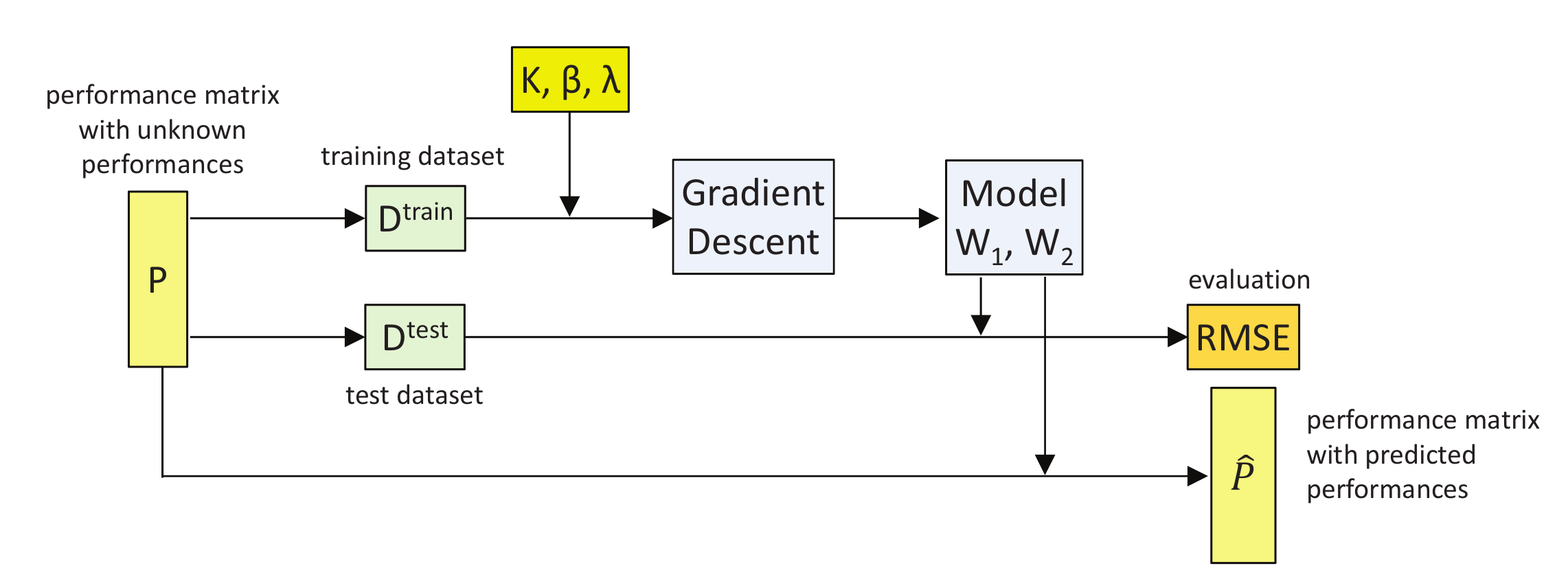
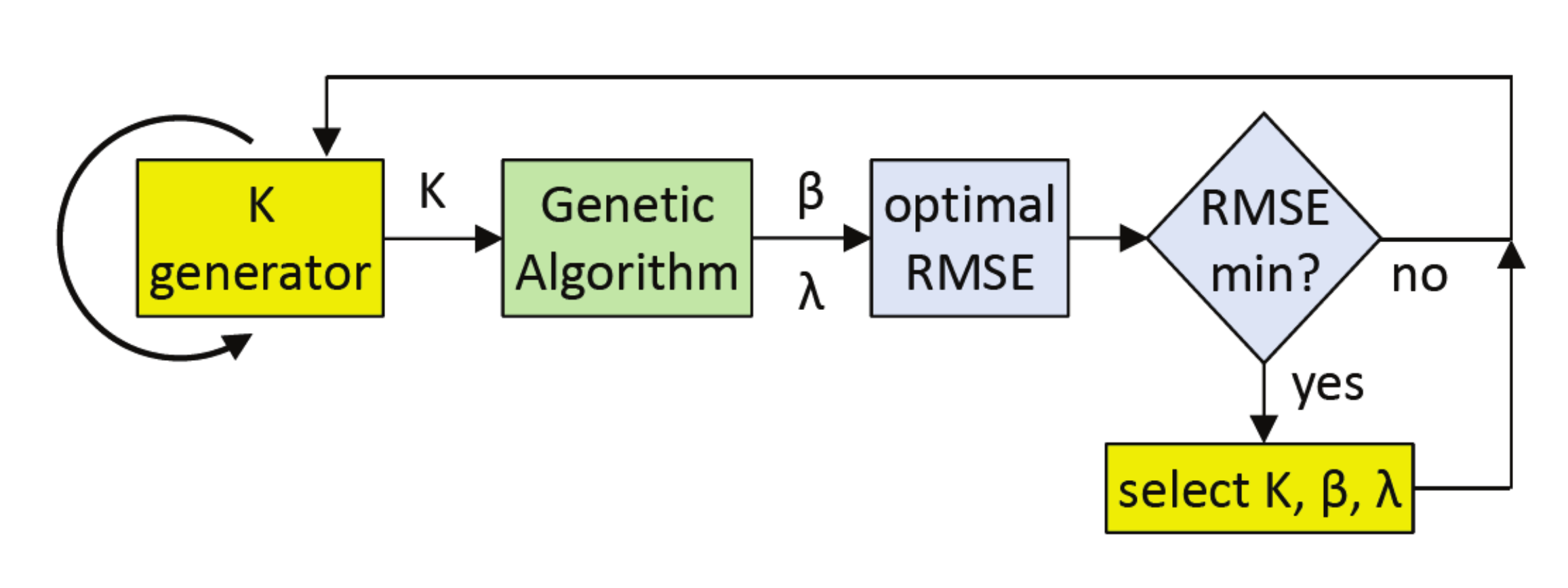
The prediction methodology follows three steps, according to the model described in [6], similar to the well-known Probabilistic Matrix Factorization (PMF) model [36]. First, we find the best parameters for $W_1$ and $W_2$ in the learning phase, through $D^{train}$, by measuring the differences between real and predicted values. Next, we check the validity of the model by predicting the values of $D^{test}$ and calculating the difference from the real values. Last, we calculate the unknown values of P from the optimal model (that with minimum $RMSE$). This process is summarized in Figure 1.

Learning the model means finding the optimal values for $W_1$ and $W_2$ iteratively. Initially, both matrices contain random values as positive real numbers generated from the normal distribution $N(0,{\sigma }^2)$. Then, we calculate the error (3) on the training dataset, where $e_{s,i}$ (4) is the error made by the prediction of $p_{s,i}$, and consequently, $e_{s,i}^2$ is calculated as in (10).

$$err=\sum _{(s,i)\in D^{train}}{e}_{s,i}^2$$

(3)

$$e_{s,i}=p_{s,i}-{\widehat{p}}_{s,i}=p_{s,i}-\sum _{k=1}^K\left(w_{1_{s,k}}{w}_{2_{i,k}}\right)$$

(4)

$$e_{s,i}^2={(p_{s,i}-\sum _{k=1}^K\left(w_{1_{s,k}}{w}_{2_{i,k}}\right))}^2$$

(5)

We can minimize the error in (10) by updating $W_1$ and $W_2$ iteratively, considering GD. This algorithm is very useful for solving problems when handling large datasets [37]. In order to apply GD, we must know, for each data point, in which direction to update the values $w_{1_{s,k}}$ and $w_{2_{i,k}}$ by calculating the gradients of $p_{s,i}$.

$$\frac{\partial }{\partial w_{1_{s,k}}}{e}_{s,i}^2=-2e_{s,i}{w}_{2_{i,k}}=-2(p_{s,i}-{\widehat{p}}_{s,i})w_{2_{i,k}}$$

(6)

$$\frac{\partial }{\partial w_{2_{i,k}}}{e}_{s,i}^2=-2e_{s,i}{w}_{1_{s,k}}=-2(p_{s,i}-{\widehat{p}}_{s,i})w_{1_{s,k}}$$

(7)

Next, we update the values $w_{1_{s,k}}$ and $w_{2_{i,k}}$ in the opposite direction to the gradient (8) and (9).

$${w^{\prime }}_{1_{s,k}}=w_{1_{s,k}}-\beta \frac{\partial }{\partial w_{1_{s,k}}}{e}_{s,i}^2=w_{1_{s,k}}+2\beta e_{s,i}{w}_{2_{i,k}}$$

(8)

$${w^{\prime }}_{2_{i,k}}=w_{2_{i,k}}-\beta \frac{\partial }{\partial w_{2_{i,k}}}{e}_{s,i}^2=w_{2_{i,k}}+2\beta e_{s,i}{w}_{1_{s,k}}$$

(9)

The updating process is iterative. It stops when a certain criterion is satisfied, for example when the error has converged to its minimum value or when a predefined number of iterations has been reached.

A new parameter appears in (8) and (9): the learning rate $\beta$, which is a positive real number, usually in the range $(0,1)$. This parameter affects the convergence of the algorithm. Therefore, several techniques were used to select the best value dynamically [38,39].

In order to prevent over-fitting, a regularization factor $\mathit{\lambda }$ is added to $e_{s,i}^2$ (10). This term also affects the accuracy of the prediction model. The newer gradients (11) and (12) update $W_1$ and $W_2$ according to (13) and (14), respectively.

$$e_{s,i}^2={(p_{s,i}-{\widehat{p}}_{s,i})}^2+\mathit{\lambda }\left(\right||W_1{\left|\right|}^2+\left|\right|W_2{\left|\right|}^2)$$

(10)

$$\frac{\partial }{\partial w_{1_{s,k}}}{e}_{s,i}^2=-2e_{s,i}{w}_{2_{i,k}}+\mathit{\lambda }{w}_{1_{s,k}}$$

(11)

$$\frac{\partial }{\partial w_{2_{i,k}}}{e}_{s,i}^2=-2e_{s,i}{w}_{1_{s,k}}+\mathit{\lambda }{w}_{2_{i,k}}$$

(12)

$${w^{\prime }}_{1_{s,k}}=w_{1_{s,k}}+\beta (2e_{s,i}{w}_{2_{i,k}}-\mathit{\lambda }{w}_{1_{s,k}})$$

(13)

$${w¡}_{2_{i,k}}=w_{2_{i,k}}+\beta (2e_{s,i}{w}_{1_{s,k}}-\mathit{\lambda }{w}_{2_{i,k}})$$

(14)

Once $W_1$ and $W_2$ are available, we calculate $RMSE$ on $D^{test}$ to assess the accuracy of the prediction model.

3.2. Training and Test Datasets

There are many strategies for selecting the training and test datasets [40]. The datasets chosen for a particular problem may eschew the performance results [41]. This is the rationale behind the particular strategy selected here, which pursues two goals.

First, we choose large-sized training datasets, comprising all the observed or known performance values. Since the size of the databases from virtual classrooms are not too big, they can be processed with the usual computer resources. Therefore, considering all the known performances as training data remains manageable.

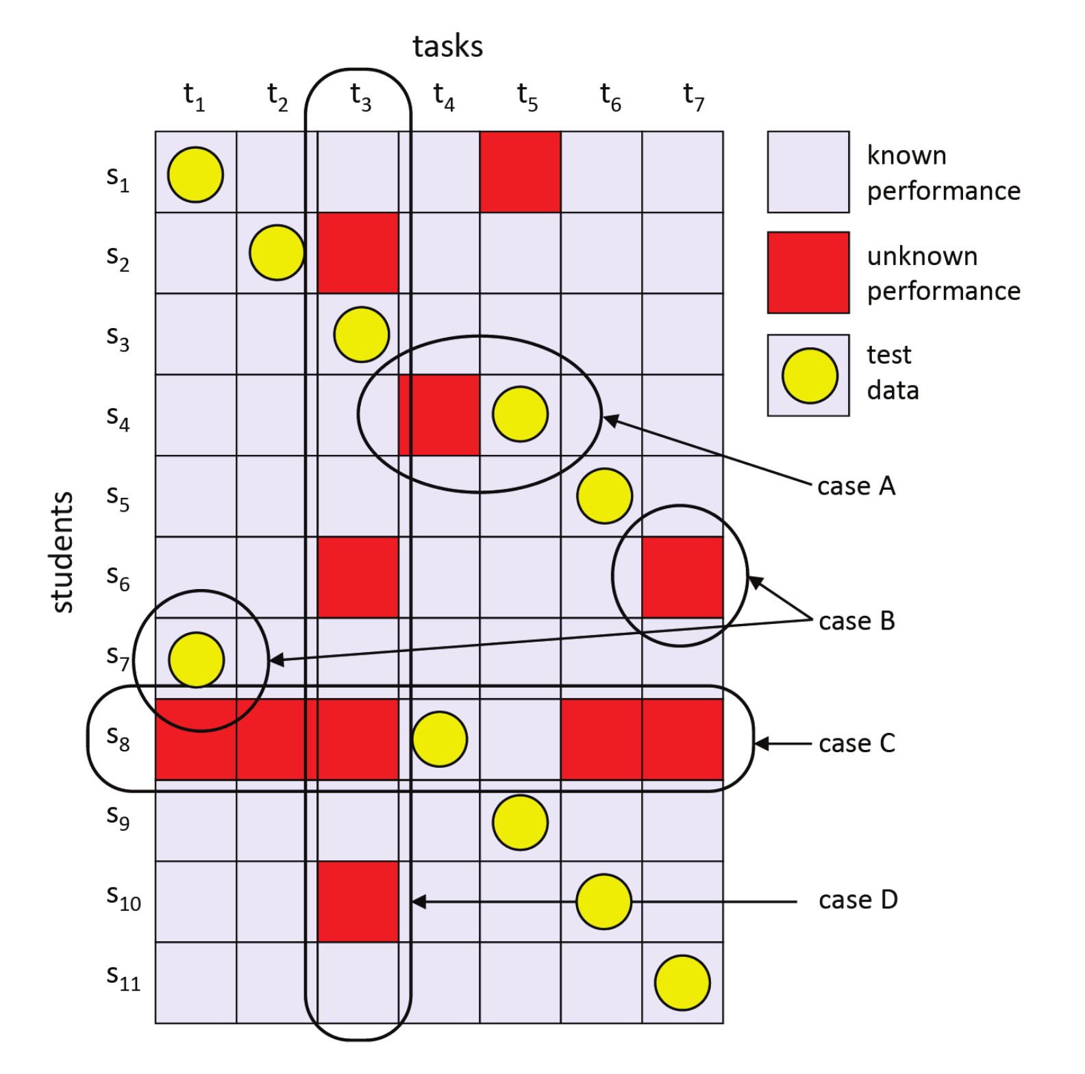
Second, we build the test dataset by selecting one performance value by each student (row) for consecutive tasks (columns). Figure 2 shows an example of this strategy. When the selected test performance is an unknown value, we skip to the next column of the same row (Case A in the figure) unless the end of the row has been reached, in which case, we select the first column of the next row (Case B in the figure). It is important to note that test data must be known data. By following this procedure, we make sure that the test data factor in all the students and all the tasks proportionately.

3.3. Data Filtering

The prediction of the unknown performance corresponding to a particular student-task binomial considers not only the performance of the student in the completed tasks, but also the performance of the remaining students for the same task, according to the collaborative filtering algorithms. Hence, it is important to remove those students and tasks that may eschew the results due to the outlying values. For example, if a student did not attend the majority of the tasks because of a lack of interest or because the subject was partially validated, s/he should not be considered for this activity because the unknown performances are not isolated, random events. By the same token, the tasks attended to by very few students are not to be considered, since it would normally mean that these tasks are not significant enough in the academic progress of the subject.

In view of the above considerations, several filters were applied to the original data extracted from a virtual classroom database. These filters ensure that the unknown performance values are due to valid reasons. Consequently, the collaborative filtering algorithms will make predictions with more possibilities of success.

We selected filters for removing the students with less than $25\%$ of academic activity completed in the subject, and only the tasks attended by at least $75\%$ of the students were considered. The dataset, obtained after applying the filters, provides a good representation of the available data in order to perform the prediction experiments. Figure 2 shows a simple case of how the filter works: student $s_8$ (Case C) with $14\%$ of activity and task $t_3$ (Case D) with $63\%$ of activity should be removed since they do not reach the minimum levels of activity required, $25\%$ and $75\%$, respectively.

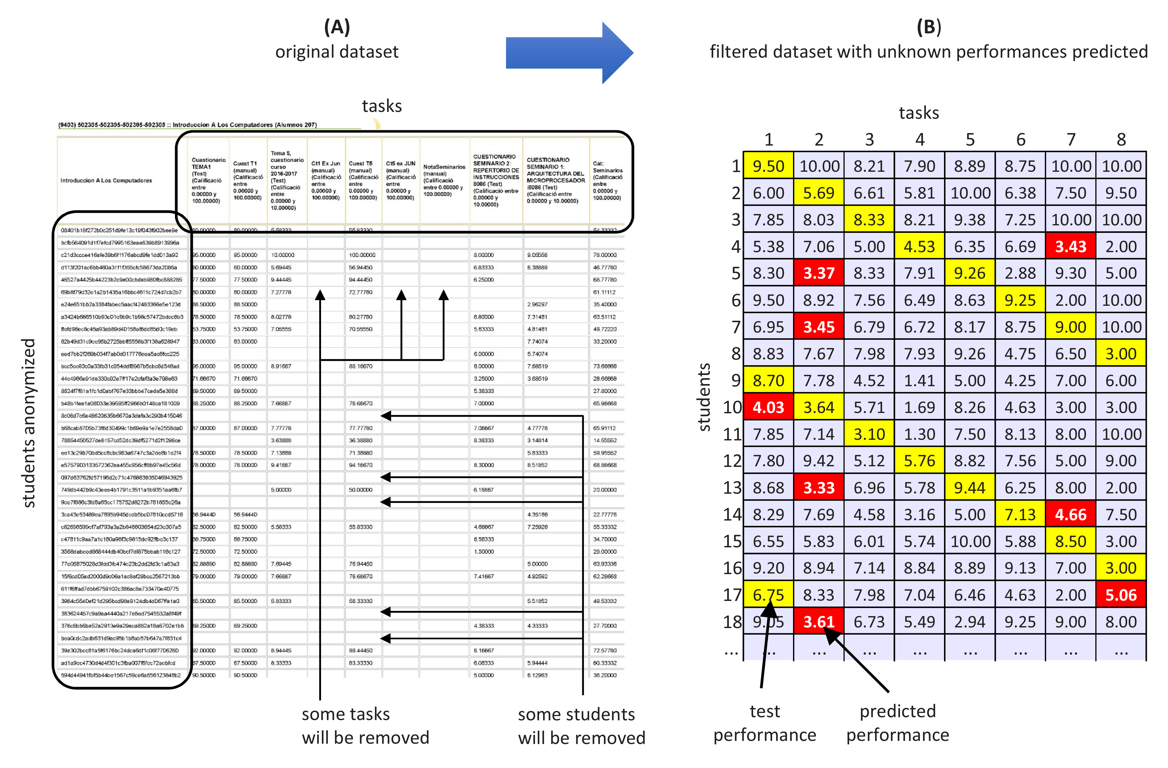
Figure 3 shows a real case of the filtering and prediction of unknown performances. It corresponds to a small virtual classroom (HS) of 128 students and 16 tasks. On the top (A), we can see a section of the performance matrix with the original data as they were collected from the corresponding database. There are some void tasks probably prepared by the teacher, but eventually not assigned to the students, and some students with a low or null level of academic activity. If we apply the prediction algorithms to this performance matrix, the contribution of those tasks and students to the prediction results is negative. Hence, we need to remove them according to the methodology outlined above.

After applying the corresponding filters, we obtain the final performance matrix, a piece of which can be seen at the bottom of (B). Now, the dataset is reduced to 95 students and five tasks that meet $60\%$ and $92\%$ of the minimum academic activity, respectively. The performance matrix contains 475 values, and eighteen of them are unknown. The training and test datasets have 457 and 92 scores respectively, according to the building rules considered in Section 3.2. In this figure, the cells show performance values from zero to 10, and black and gray cells represent unknown and test scores, respectively.

Finally, the model predicted the unknown performances, whose values appear in the bottom picture. These values were calculated considering $K=64$ latent factors, $\beta =0.8$, and $\mathit{\lambda }=0.06$, from which we obtained $RMSE=0.37$.

Note that the prediction considers not only the performance of the student in the completed tasks, but also the performance of the remaining students for the same task. Consequently, we can study the expected behavior of each student by analyzing the predictions in order to detect the strengths and weaknesses of the learning process in the corresponding subject.

4. Proposal for Improving The Prediction

We identified three parameters that affect the prediction accuracy measured as $RMSE$: the number of latent factors (K), the learning rate ($\beta$), and the regularization factor ($\mathit{\lambda }$). We can improve the prediction by finding the optimal values for these parameters that minimize $RMSE$, for a given dataset.

4.1. Efficient Tuning of Collaborative Filtering

In order to show the influence of $\beta$ and $\mathit{\lambda }$ on the prediction accuracy, given a particular number of latent factors, we apply Direct Search (DS). DS is a very simple approach to obtain the optimal pair of values ($\beta$, $\mathit{\lambda }$) among a set of pairs taken from predefined sets for both parameters. Each of $\beta$’s and $\mathit{\lambda }$’s values grow by incremental steps $h_{\beta }$ and $h_{\mathit{\lambda }}$, respectively, from the minimum ${\beta }_{min}$ and ${\mathit{\lambda }}_{min}$ to the maximum ${\beta }_{max}$ and ${\mathit{\lambda }}_{max}$ values, respectively. The search is implemented by two nested loops, where $RMSE$ is calculated for each generated pair.

This method has the disadvantage of limiting the number of evaluated pairs ($\beta$, $\mathit{\lambda }$), since it is directly related to the computing effort that can be made. Because of this, better values could have been ignored and not considered in the search; however, DS allows one to find a good solution among the ones that have been generated, which may lie in the vicinity of the potentially optimal solutions.

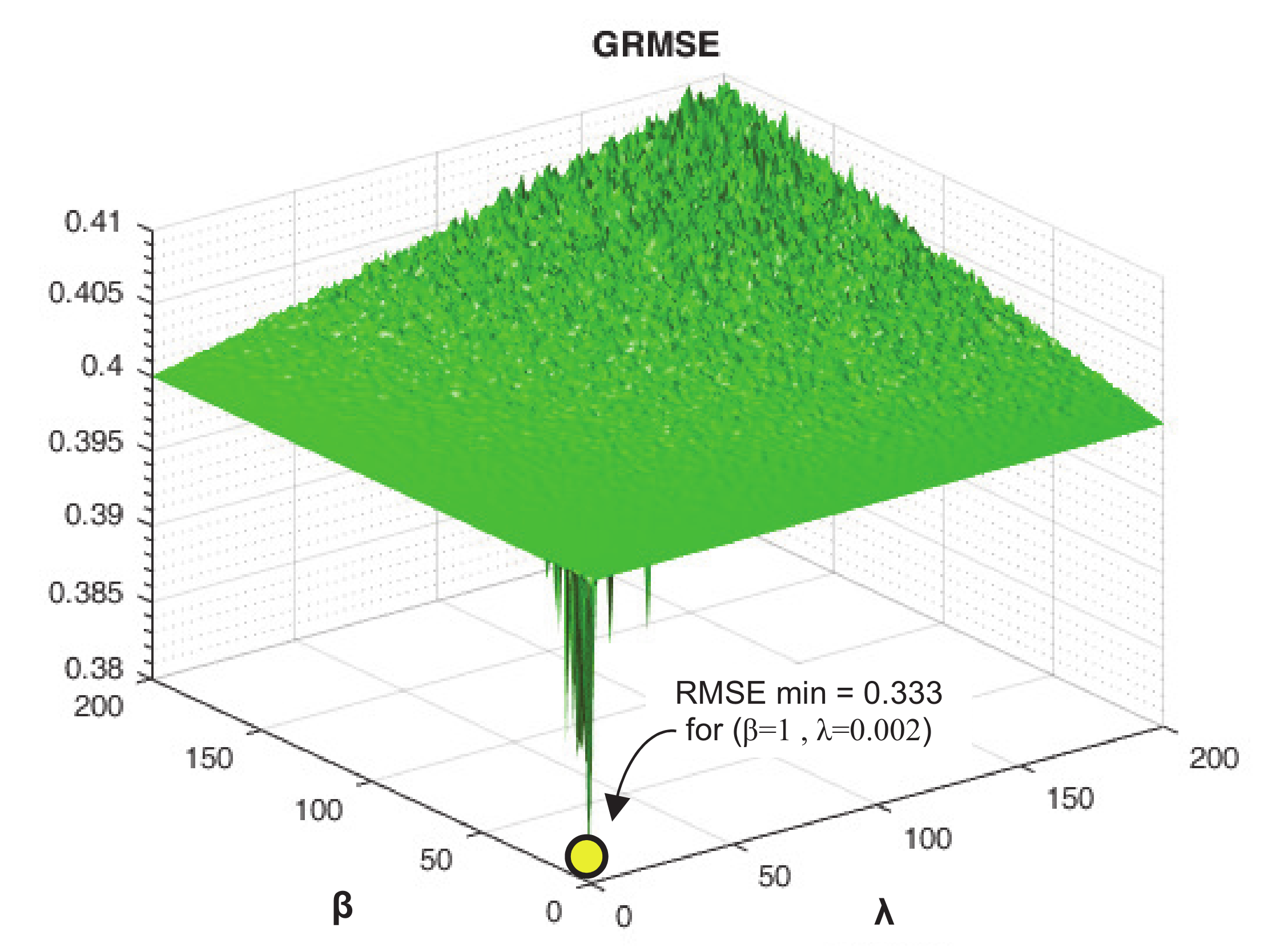
Figure 4 shows an example of DS, where a dataset composed of 107 students and eight tasks was processed, applying predictions for 56 unknown scores, considering the ranges $0.1<\beta <200$ and $0.001<\mathit{\lambda }<200$. The 209 and 227 values for $\beta$ and $\mathit{\lambda }$, respectively, were extracted at equal intervals from these ranges. In total, forty-seven-thousand four-hundred forty-three values of $RMSE$ were calculated, obtaining a minimum value of $0.333$ (yellow circle on the plot), which corresponded to $\beta =1$ and $\mathit{\lambda }=0.002$. The predictions considered $K=64$ latent factors.

This figure displays the $GRMSE$ metric for each pair ($\beta$,$\mathit{\lambda }$). This metric is the same $RMSE$ after applying a linear function that highlights the minimum points, maintaining the proportion among all the points, in order to make minimums easier to detect on the plot. The evidence of several minimum points suggests that the prediction accuracy is very sensitive to the selected pair, so we would need to perform a deeper search. Nevertheless, DS wastes much computational effort when searching in wide areas without minimum values of $RMSE$. This consideration led us to suggest more efficient optimization alternatives in order to find the value of K and the pair ($\beta$,$\mathit{\lambda }$) for which $RMSE$ is minimum.

4.1.1. Optimization Techniques

As there are no solid methods to determine the optimal values for K, $\beta$ and $\mathit{\lambda }$, we tackled this problem by applying two optimization techniques: genetic algorithms and pattern search.

4.1.2. Genetic Algorithm

Metaheuristics [42] are approximate algorithms that explore the space of solutions efficiently, by focusing the search on the vicinity of a promising solution. This is the rationale behind the application of metaheuristics to solve large optimization problems. Metaheuristics are classified as trajectory or population algorithms. Among population- based metaheuristics, Evolutionary Algorithms (EAs) [43] search the optimal solutions by tracing the evolution of individuals according to rules inspired by biological phenomena.

Genetic Algorithms (GAs) [44] are popular EAs that perform stochastic searches after postulating an individual solution to the optimization problem. The individual X is composed of several decision variables $x_i$ that define its genotype. In our case, we have two decision variables: $x_1=\beta$ and $x_2=\mathit{\lambda }$. A population is a set of individuals that evolves along generations. The genetic pool of the population is composed of the genotypes of their individuals. The population evolves by minimizing a fitness function $f\left(X\right)$; in our problem, it is $RMSE$.

GA starts generating an initial population and evaluating its individuals. From here on, the population evolves along generations. Each generation consists of several sequential phases. The first phase assigns a fitness value to each individual. Next, the selection phase chooses the best individuals (parents) for crossover according to their fitness values. The third phase (recombination) crosses the parents to generate new individuals (offspring), thus updating their fitness values. After that, some individuals among the offspring develop mutations, their fitness being updated accordingly. The evaluation phase evaluates the offspring and eventually incorporates it back into the population (reinsertion phase). Then, the assignment phase starts again in order for the next generation to begin. The GA ends when it reaches a stopping criterion (usually a predefined number of generations).

The GA was tuned for the experiments by selecting the following values for the main hyper-parameters, among others: population size of 150 individuals; 60 generations as the stopping criterion; (0.0001,10) as the range of search for $\beta$; (0.0001,1) as the range of search for $\mathit{\lambda }$; (2,200) as the range of search for K; random initial population with a uniform distribution; rank as the fitness scaling function; stochastic uniform as the selection function; scattered crossover function; elite count (number of individuals that are guaranteed to survive to the next generation) of $5\%$ of the population size; crossover fraction of 0.8; Gaussian mutation function; and 31 runs for each experiment.

4.1.3. Pattern Search

Pattern Search (PS) [45] is a direct search method for solving optimization problems. Unlike other optimization algorithms, PS does not require any information about the gradient or higher derivatives of the $RMSE$ function when searching for an optimal set of optimization parameters (in our case, K, $\beta$, and $\mathit{\lambda }$), but it searches a set of values of the optimization parameters around the current set, looking for one where the value of $RMSE$ is lower than the value at the current set.

In other words, PS is a pattern search algorithm that computes the $RMSE$ corresponding to a sequence of sets of the optimization parameters that approach an optimal set. At each step, PS searches a mesh, around the current set (obtained at the previous step of the algorithm). The mesh is built from adding the current set to a scalar multiple of a set of vectors called a pattern. If PS finds a set in the mesh that improves $RMSE$ at the current set, the new set becomes the current set at the next step of the algorithm.

4.2. Three Approaches for The Optimization

In light of a DS approach, it is necessary to keep in mind two considerations. First, there are many different possibilities when selecting the values of the pair ($\beta$, $\mathit{\lambda }$), since they are real numbers chosen from different ranges, where the precision of the floating point values can be important. On the contrary, there are not many possible values for K since it is an integer number chosen from a relatively restricted range, for example between two and 256 [6] in the PSP context. Therefore, we propose three approaches for solving the optimization problem of finding the optimal values of K, $\beta$, and $\mathit{\lambda }$ for which $RMSE$ is minimum:

• GAK: This method implements a loop of predictions where for each K value, the GA algorithm is applied in order to obtain the optimal pair ($\beta$, $\mathit{\lambda }$), as outlined in Figure 5. This way, the minimum $RMSE$ found would correspond to the optimal values of K, $\beta$, and $\mathit{\lambda }$.
• GA3: This method applies the same GA algorithm than in GAK, but including K as the third optimization parameter. This way, there is no need for a K loop, since GA optimizes in each run the three parameters K, $\beta$, and $\mathit{\lambda }$ together.
• PS3: This method follows the same idea as GA3, although replacing GA by PS as the optimization algorithm.

5. Experimental Results

In this section, we show the experimental results after applying the three optimization methods GAK, GA3, and PS3, considering different datasets, each of them extracted from virtual classrooms. For each framework (dataset), the optimal solution is given by such a value of K that the best $RMSE$ found was minimum, as were the corresponding values of $\beta$ and $\mathit{\lambda }$.

5.1. Datasets

We built several datasets to perform the experiments of predicting students’ performance. They are available at the Mendeley Data repository [46]. These datasets were prepared from virtual classrooms of a series of university-level courses, the data of which were adequately filtered according to the method explained in Section 3.3. The purpose of preparing this suite of datasets was having different cases for different academic contexts: number of students and tasks, degree levels (first, middle, or final years), academic nature (theoretical or practical contents), etc. This heterogeneous suite also contributes to considering a different number of latent factors, which is important in order to test the optimization algorithms proposed in Section 4.

The virtual classrooms of the online campus of the University of Extremadura (UEX) provided the necessary data for the datasets. This online campus is composed of several software services working together in order to cater to the needs of the users:

• Portal: It welcomes users and allows them to log in. It also implements the only communication channel between the users and tech support.
• Avuex: It consists of a large set of virtual classrooms corresponding to the different bachelor’s and master’s degrees, oriented toward the learning process.
• Evuex: It consists of a set of virtual spaces oriented toward different purposes for the university community (short courses, seminars, workshops, etc.).

Table 2. Experimental datasets.

Dataset	IC	HS	TO	EN	BE	PR	SR	SJ
Virtual	Introduction	Food Hygiene	Clinical	Women’s	Biostatistics for	Internet	Network	Youth
Classroom	to Computers	and Safety	Toxicology	Nursing	Biotechnology	Programming	Security	Subcultures
	Original data
S (students)	207	128	123	90	47	78	17	26
I (tasks)	38	16	6	18	30	17	24	6
P (scores)	7866	2048	738	1620	1410	1326	408	156
	Filtered data
S (students)	107	95	116	78	47	65	10	26
I (tasks)	8	5	3	9	10	2	24	6
P (scores)	7856	475	348	702	470	130	240	156
	Subsets
$D^{knw}$ (known data)	800	457	324	657	440	116	214	155
$D^{unk}$ (unknown data)	56	18	24	45	30	14	26	1
$D^{train}$ (training data)	800	457	324	657	440	116	214	155
$D^{test}$ (test data)	102	92	105	73	43	59	19	26
	Minimum activity level
Students ${}^1$	88%	60%	33%	78%	30%	50%	50%	83%
Tasks ${}^2$	80%	92%	86%	77%	89%	78%	75%	96%

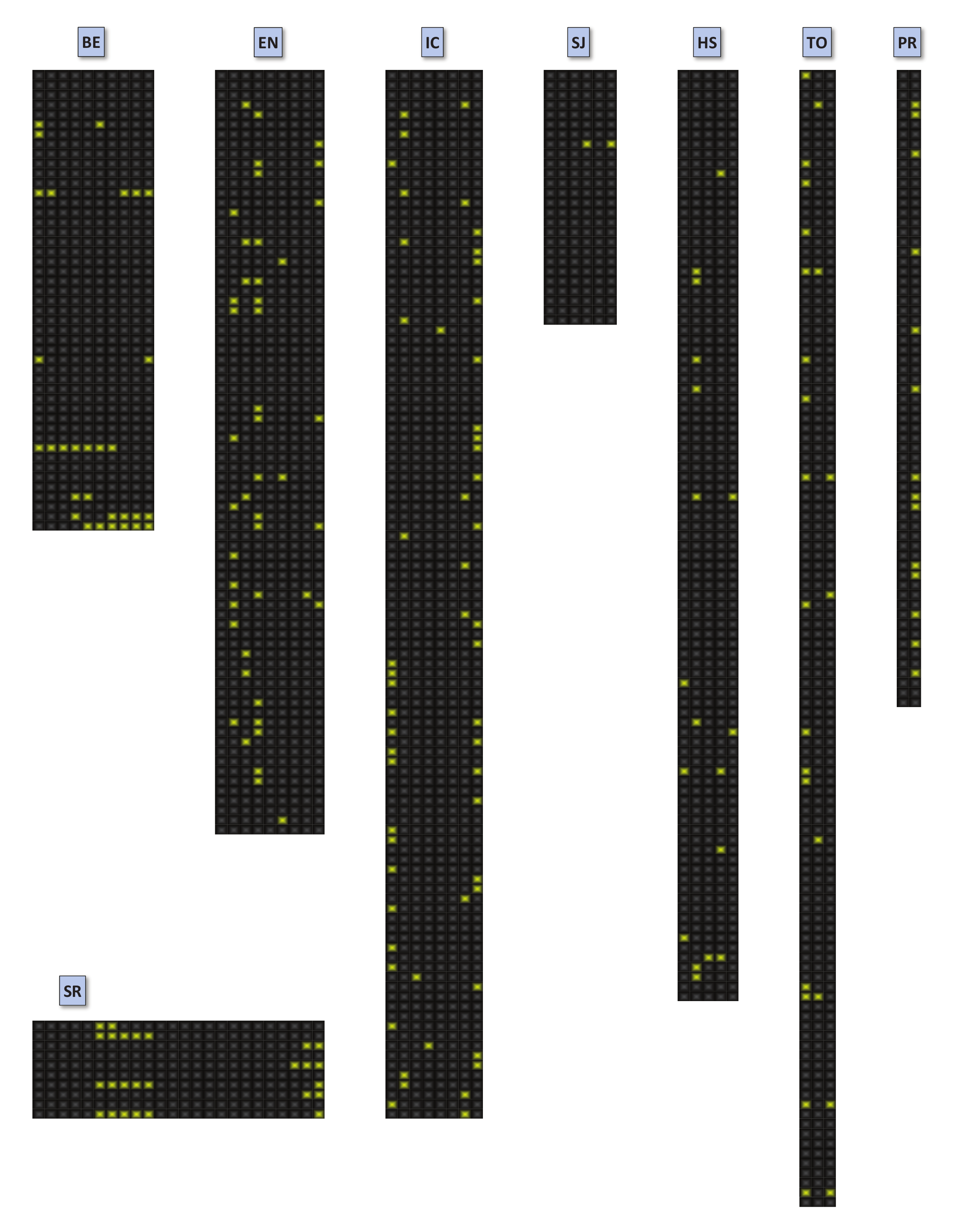
¹ Greater than or equal to 25%, ² Greater than or equal to 75%.

shows the datasets corresponding to eight virtual classrooms. It lists the number of students (S), tasks (I), the performance matrix (P) before (original data) and after (filtered data) the filtering process, the number of known ($D^{knw}$) and unknown ($D^{unk}$) performances, the sizes of the training ($D^{train}$) and test ($D^{test}$) datasets, and the percentages of the minimum activity levels for students and tasks allowed by the filtering method. Besides, we can see in Figure 6 the variety of shapes and of the eight datasets. The number and location of the unknown performances are highlighted. This variety of features allows the algorithms to demonstrate their effectiveness in different scenarios.

5.2. Accuracy Analysis and Discussion

The experimental method for GAK consisted of selecting several consecutive values of K, from two to 160, in an iterative process where for each K, a GA experiment was performed. In each iteration, the GA experiment involved several runs, since GA has a strong non-deterministic nature, where the best run reported the minimum $RMSE$. Once all the iterations were completed, we pointed out the iteration (K value) for which $RMSE$ was the minimum among the best ones and the corresponding pair ($\beta$, $\mathit{\lambda }$). On the contrary, the experimental method for GA3 and PS3 considers simply applying GA and PS where each individual in the population is composed of three values corresponding to the optimization parameters K, $\beta$, and $\mathit{\lambda }$.

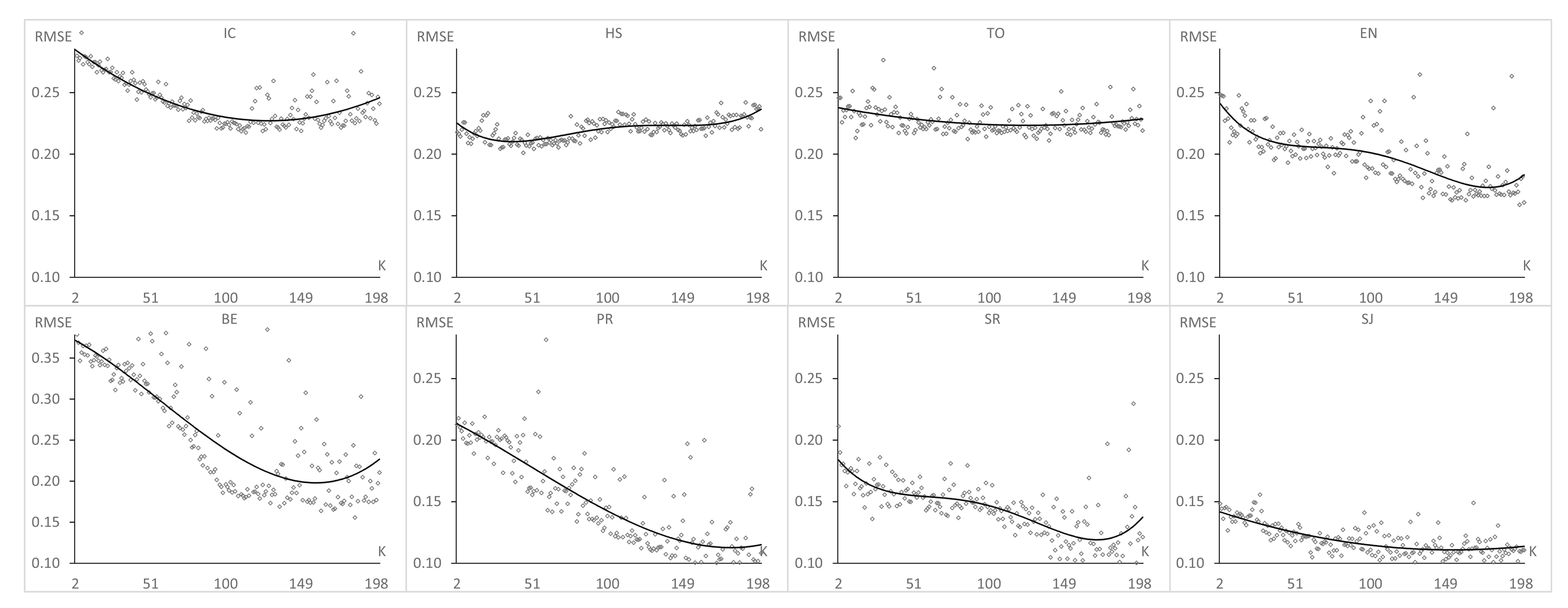
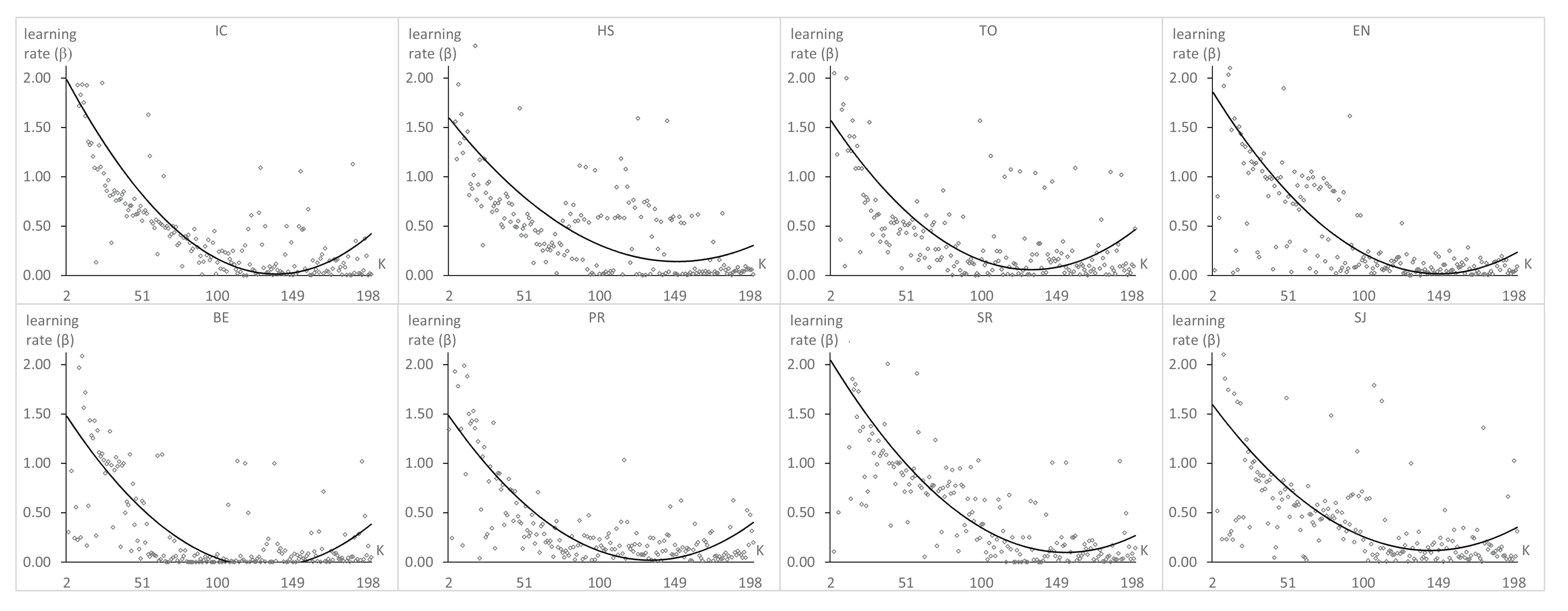
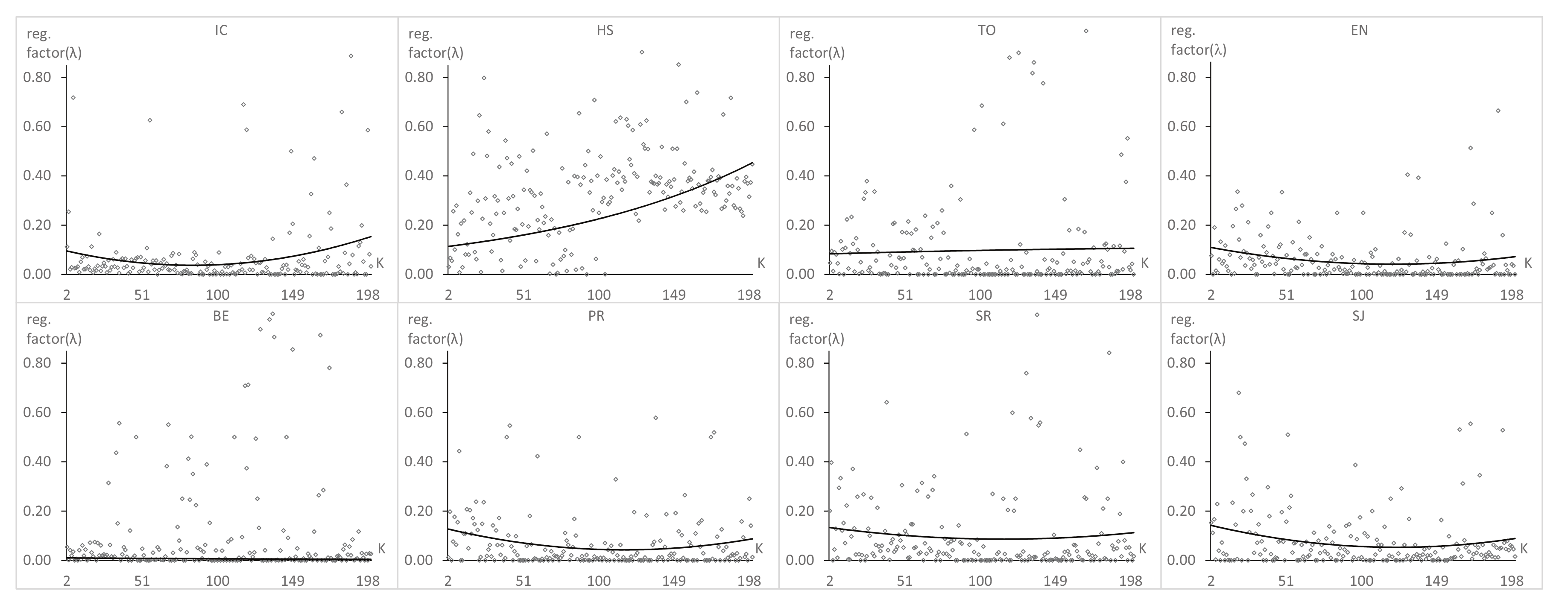
Figure 7, Figure 8 and Figure 9 show the results of $RMSE$, $\beta$, and $\mathit{\lambda }$, respectively, obtained after applying GAK for each value of K from two to 200, considering the eight datasets described in the previous section.

Table 3. Results for the optimization method GAK.

GAK	$\mathbf{RMSE}$	Values for $\mathit{R}\mathit{M}\mathit{S}\mathit{E}$ min
Dataset	min	$\mathit{\beta }$	$\mathit{\lambda }$	K
IC	0.218	0.022	0.0070	113
HS	0.201	0.495	0.1841	45
TO	0.211	0.077	0.0001	139
EN	0.159	0.037	0.0001	197
BE	0.156	0.010	0.0001	184
PR	0.089	0.033	0.0001	153
SR	0.092	0.044	0.0098	192
SJ	0.097	0.052	0.0001	139

shows the optimal values found after applying the GAK method.

There are two significant conclusions to be drawn after analyzing the GAK plots. First, the plots of $RMSE$ have a similar behavior. For each dataset, there is only one optimal value of K. Until this value is reached, $RMSE$ decreases when K increases; after it has been reached, the reverse occurs. Second, the optimal K values depend strongly on the considered dataset; however, they are in the range between 45 and 197. This way, we could select a value in the middle of this range to be used by default for general experiments in PSP when the optimal number of latent factors for a particular dataset is unknown, provided that it is comparable in size to the dataset that has been used here. Furthermore, we can check that $\beta$ follows a similar trend as $RMSE$ when K increases, while $\mathit{\lambda }$ does not show a particular behavior.

Table 4. Results for the optimization method GA3.

GA3	$\mathit{R}\mathit{M}\mathit{S}\mathit{E}$					Values for $\mathit{R}\mathit{M}\mathit{S}\mathit{E}$ min
Dataset	min	max	Mean	dev.st.	Median	$\mathit{\beta }$	$\mathit{\lambda }$	K
IC	0.230	0.263	0.248	9.04× ${10}^{-3}$	0.248	0.204	0.019	106
HS	0.215	0.277	0.234	1.22× ${10}^{-2}$	0.233	0.540	0.339	55
TO	0.238	0.276	0.255	1.03× ${10}^{-2}$	0.254	0.020	0.002	136
EN	0.179	0.295	0.207	2.03× ${10}^{-2}$	0.206	0.008	0.001	187
BE	0.179	0.239	0.209	1.58× ${10}^{-2}$	0.207	0.003	0.133	153
PR	0.107	0.174	0.133	1.42× ${10}^{-2}$	0.131	0.016	0.003	194
SR	0.144	0.200	0.169	1.51× ${10}^{-2}$	0.167	0.007	0.006	188
SJ	0.129	0.182	0.148	1.30× ${10}^{-2}$	0.147	0.129	0.002	159

and

Table 5. Results for the optimization method PS3.

PS3	$\mathit{R}\mathit{M}\mathit{S}\mathit{E}$					Values for $\mathit{R}\mathit{M}\mathit{S}\mathit{E}$ min
Dataset	min	max	Mean	dev.st.	Median	$\mathit{\beta }$	$\mathit{\lambda }$	K
IC	0.23	2.74	0.50	5.87× ${10}^{-1}$	0.26	0.235	0.011	114
HS	0.21	3.82	0.87	8.74× ${10}^{-1}$	0.32	0.651	0.141	29
TO	0.22	9.50	1.20	2.02	0.28	0.040	0.013	183
EN	0.18	2.31	0.53	5.02× ${10}^{-1}$	0.27	0.049	0.004	163
BE	0.16	2.89	0.51	5.42× ${10}^{-1}$	0.37	0.001	0.171	195
PR	0.10	4.19	1.08	1.46	0.22	0.003	0.014	197
SR	0.11	2.11	0.47	5.52× ${10}^{-1}$	0.24	0.043	0.000	168
SJ	0.11	54.65	2.34	9.72	0.48	0.068	0.010	176

show the main results after applying the GA3 and PS3 methods, respectively. As the optimization problem has a strong non-deterministic nature, each experiment of GA and PS consisted of 31 runs. Therefore, the minimum, maximum, mean, median, and standard deviation are shown. The optimal values of the parameters K, $\beta$, and $\mathit{\lambda }$ correspond to the minimum value of the $RMSE$ found in each experiment.

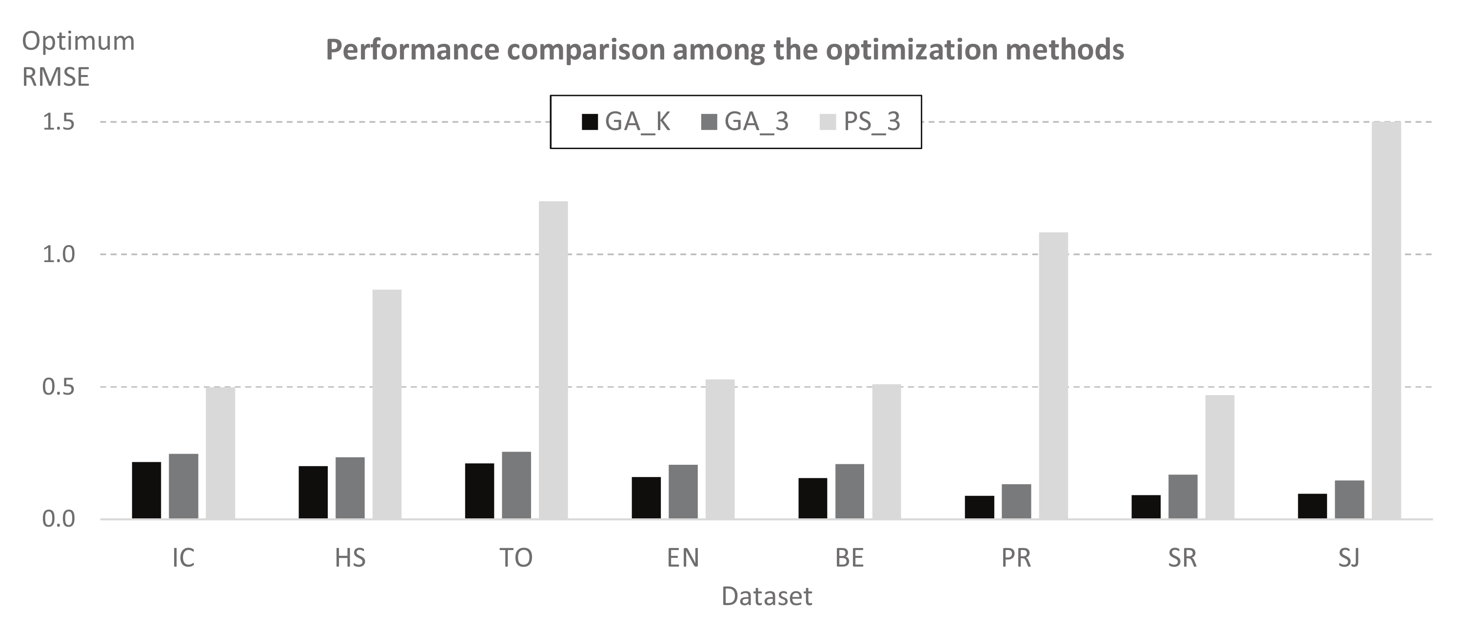
As we applied three optimization methods for solving the PSP problem, we can analyze the performance of these methods by comparing the minimum $RMSE$ found for each dataset. Figure 10 shows the optimal values of $RMSE$ collected from Table 3, Table 4 and Table 5. We check that the GAK method outperforms the prediction accuracy provided by GA3 and PS3 for all the datasets considered. In other words, including K as a third optimization parameter in GA and PS does not improve the prediction accuracy. Furthermore, we can also conclude that GA provides better results than PS, regardless of whether we consider K as an optimization parameter.

6. Conclusions

We focused our research on improving the prediction accuracy of the students’ performance when applying a method based on collaborative filtering to datasets extracted from virtual classrooms in online campuses. This method makes use of a technique used in recommender systems to predict unknown performances and building models by using matrix factorization and the gradient descent algorithm.

The prediction of the unknown performances is very useful for students and teachers from the learning point of view. On the one hand, students can predict the score of an unfinished or un-attended task, according to the scores of their completed tasks and the scores of their colleagues who completed the task in question. This prediction can help the student to identify the main strengths or weaknesses in their learning process of the corresponding subject and provide insights about how to maximize the study effort. On the other hand, the teacher can monitor the level of success for a particular task by recording the performance of all the students, including the predictions of the unknown scores.

The particular nature of each virtual classroom (number of students and tasks, degree, type of learning) involves considering a different number of latent factors. We have proven that selecting a right number of latent factors, together with optimal values for the learning rate and regularization factor, improves the prediction accuracy by minimizing the error in the prediction of the test dataset. Our proposal consists of optimizing these three parameters by applying a direct search of the ideal number of latent factors at the same time that the prediction model is optimized by means of a genetic algorithm, thus obtaining a minimum prediction error.

The experimental framework consisted of eight real-world datasets, filtered accordingly for a realistic processing. After applying the proposed optimization method, not only did this method outdo the prediction accuracy when compared to using simple direct search for the optimal values of $\beta$ and $\mathit{\lambda }$ with less computing time, it also obtained a range where to locate the ideal number of latent factors. The mean value of the number of latent factors can be found within this range; and it can be utilized by default for prediction purposes on other datasets, without having to perform previous optimization experiments.

The importance of PSP and the results obtained in this work encourage us to consider other techniques to improve the accuracy of the prediction. In this line, other ML methods can be explored and compared.

References

- Coccoli, M.; Maresca, P.; Molinari, A. Collaborative E-learning Environments with Cognitive Computing and Big Data. J. Vis. Lang. Comput. 2019, 2019, 43–52. [Google Scholar] [CrossRef]
- Murphy, K.P. Machine Learning: A Probabilistic Perspective; The MIT Press: Cambridge, MA, USA, 2012. [Google Scholar]
- Wu, X.; Zhu, X.; Wu, G.; Ding, W. Data mining with big data. IEEE Trans. Knowl. Data Eng. 2014, 26, 97–107. [Google Scholar] [CrossRef]
- Alpaydin, E. Introduction to Machine Learning; The MIT Press: Cambridge, MA, USA, 2014. [Google Scholar]
- Jannach, D.; Zanker, M.; Felfernig, A.; Friedrich, G. Recommender Systems. An Introduction; Cambridge University Press: Cambridge, UK, 2011. [Google Scholar]
- Thai-Nghe, N.; Drumond, L.; Horvath, T.; Krohn-Grimberghe, A.; Nanopoulos, A.; Schmidt-Thieme, L. Factorization Techniques for Predicting Student Performance. In Educational Recommender Systems and Technologies: Practices and Challenges; IGI-Global: Hershey, PA, USA, 2012; pp. 129–153. [Google Scholar]
- Koren, Y.; Bell, R.; Volinsky, C. Matrix Factorization Techniques for Recommender Systems. Computer 2009, 42, 30–37. [Google Scholar] [CrossRef]
- Koren, Y. Factor in the Neighbors: Scalable and Accurate Collaborative Filtering. ACM Trans. Knowl. Discov. Data 2010, 4, 1–24. [Google Scholar] [CrossRef]
- Roy, S.; Garg, A. Analyzing performance of students by using data mining techniques a literature survey. In Proceedings of the 2017 4th IEEE Uttar Pradesh Section International Conference on Electrical, Computer and Electronics (UPCON), Mathura, India, 26–28 October 2017; IEEE: Piscataway, NJ, USA, 2018; pp. 130–133. [Google Scholar] [CrossRef]
- Halde, R. Application of Machine Learning algorithms for betterment in education system. In Proceedings of the 2016 International Conference on Automatic Control and Dynamic Optimization Techniques (ICACDOT), Pune, India, 9–10 September 2016; IEEE: Piscataway, NJ, USA, 2017; pp. 1110–1114. [Google Scholar] [CrossRef]
- Anand, V.; Abdul Rahiman, S.; Ben George, E.; Huda, A. Recursive clustering technique for students’ performance evaluation in programming courses. In Proceedings of the 2018 Majan International Conference (MIC), Muscat, Oman, 19–20 March 2018; pp. 1–5. [Google Scholar] [CrossRef]
- Pushpa, S.; Manjunath, T.; Mrunal, T.; Singh, A.; Suhas, C. Class result prediction using machine learning. In Proceedings of the 2017 International Conference On Smart Technologies For Smart Nation (SmartTechCon), Bangalore, India, 17–19 August 2017; IEEE: Piscataway, NJ, USA, 2018; pp. 1208–1212. [Google Scholar] [CrossRef]
- Howard, E.; Meehan, M.; Parnell, A. Contrasting prediction methods for early warning systems at undergraduate level. Int. High. Educ. 2018, 37, 66–75. [Google Scholar] [CrossRef] [Green Version]
- Chen, Y.; Johri, A.; Rangwala, H. Running out of STEM: A comparative study across STEM majors of college students At-Risk of dropping out early. In Proceedings of the 8th international conference on learning analytics and knowledge, Sydney, Australia, 7–9 March 2018; pp. 270–279. [Google Scholar]
- Hussain, M.; Zhu, W.; Zhang, W.; Abidi, S.; Ali, S. Using machine learning to predict student difficulties from learning session data. Artif. Intell. Rev. 2018, 1–27. [Google Scholar] [CrossRef]
- Backenköhler, M.; Wolf, V. Student performance prediction and optimal course selection: An MDP approach. In Lecture Notes in Computer Science (including subseries Lecture Notes in Artificial Intelligence and Lecture Notes in Bioinformatics); 10729 LNCS; Springer: Berlin/Heidelberg, Germany, 2018; pp. 40–47. [Google Scholar]
- Sultana, S.; Khan, S.; Abbas, M. Predicting performance of electrical engineering students using cognitive and non-cognitive features for identification of potential dropouts. Int. J. Electr. Eng. Educ. 2017, 54, 105–118. [Google Scholar] [CrossRef]
- Colace, F.; De Santo, M.; Lombardi, M.; Pascale, F.; Pietrosanto, A.; Lemma, S. Chatbot for e-learning: A case of study. Int. J. Mech. Eng. Robot. Res. 2018, 7, 528–533. [Google Scholar] [CrossRef]
- Adán-Coello, J.; Tobar, C. Using collaborative filtering algorithms for predicting student performance. In Lecture Notes in Computer Science (including subseries Lecture Notes in Artificial Intelligence and Lecture Notes in Bioinformatics); 9831 LNCS; Springer: Berlin/Heidelberg, Germany, 2016; pp. 206–218. [Google Scholar]
- Baker, R.S.J.d.; Corbett, A.T.; Aleven, V. More Accurate Student Modeling through Contextual Estimation of Slip and Guess Probabilities in Bayesian Knowledge Tracing. In Intelligent Tutoring Systems; Woolf, B.P., Aïmeur, E., Nkambou, R., Lajoie, S., Eds.; Springer: Berlin/Heidelberg, Germany, 2008; pp. 406–415. [Google Scholar]
- Nespereira, C.; Elhariri, E.; El-Bendary, N.; Vilas, A.; Redondo, R. Machine learning based classification approach for predicting students performance in blended learning. Adv. Intell. Syst. Comput. 2016, 407, 47–56. [Google Scholar]
- Guo, B.; Zhang, R.; Xu, G.; Shi, C.; Yang, L. Predicting Students Performance in Educational Data Mining. In Proceedings of the 2015 International Symposium on Educational Technology (ISET), Wuhan, China, 27–29 July 2015; IEEE: Piscataway, NJ, USA, 2015; pp. 125–128. [Google Scholar] [CrossRef]
- Shanthini, A.; Vinodhini, G.; Chandrasekaran, R. Predicting students’ academic performance in the University using meta decision tree classifiers. J. Comput. Sci. 2018, 14, 654–662. [Google Scholar] [CrossRef] [Green Version]
- Rana, S.; Garg, R. Prediction of students performance of an institute using ClassificationViaClustering and ClassificationViaRegression. Adv. Intell. Syst. Comput. 2017, 508, 333–343. [Google Scholar]
- Khadiev, K.; Zulfat, M.; Sidikov, M. Collaborative filtering approach in adaptive learning. Int. J. Pharm. Technol. 2016, 8, 15124–15132. [Google Scholar]
- Sweeney, M.; Lester, J.; Rangwala, H. Next-term student grade prediction. In Proceedings of the 2015 IEEE International Conference on Big Data (Big Data), Santa Clara, CA, USA, 29 October–1 November 2015; IEEE: Piscataway, NJ, USA, 2015; pp. 970–975. [Google Scholar] [CrossRef]
- Bydžovská, H. Student performance prediction using collaborative filtering methods. Lect. Notes Comput. Sci. 2015, 9112, 550–553. [Google Scholar]
- Chavarriaga, O.; Florian-Gaviria, B.; Oswaldo Solarte, P. Recommender system based on student competencies assessment results. In Proceedings of the 2014 9th Computing Colombian Conference (9CCC), Pereira, Colombia, 3–5 September 2014; pp. 103–108. [Google Scholar] [CrossRef]
- Kuo, H.C.; Burnard, P.; McLellan, R.; Cheng, Y.Y.; Wu, J.J. The development of indicators for creativity education and a questionnaire to evaluate its delivery and practice. Think. Ski. Creat. 2017, 24, 186–198. [Google Scholar] [CrossRef]
- Lockwood, J.; Savitsky, T.; McCaffrey, D. Inferring constructs of effective teaching from classroom observations: An application of Bayesian exploratory factor analysis without restrictions. Ann. Appl. Stat. 2015, 9, 1484–1509. [Google Scholar] [CrossRef]
- Orpinas, P.; Raczynski, K.; Peters, J.; Colman, L.; Bandalos, D. Latent profile analysis of sixth graders based on teacher ratings: Association with school dropout. Sch. Psychol. Q. 2015, 30, 577–592. [Google Scholar] [CrossRef]
- Virtanen, T.; Lerkkanen, M.K.; Poikkeus, A.M.; Kuorelahti, M. Student Engagement and School Burnout in Finnish Lower-Secondary Schools: Latent Profile Analysis. Scand. J. Educ. Res. 2018, 62, 519–537. [Google Scholar] [CrossRef]
- Gaertner, H.; Brunner, M. Once good teaching, always good teaching? The differential stability of student perceptions of teaching quality. Educ. Assess. Eval. Account. 2018, 30, 159–182. [Google Scholar] [CrossRef]
- Le, T.; Bolt, D.; Camburn, E.; Goff, P.; Rohe, K. Latent Factors in Student–Teacher Interaction Factor Analysis. J. Educ. Behav. Stat. 2017, 42, 115–144. [Google Scholar] [CrossRef]
- Wagner, W.; Göllner, R.; Werth, S.; Voss, T.; Schmitz, B.; Trautwein, U. Student and Teacher Ratings of Instructional Quality: Consistency of Ratings Over Time, Agreement, and Predictive Power. J. Educ. Psychol. 2016, 108, 705–721. [Google Scholar] [CrossRef]
- Salakhutdinov, R.; Mnih, A. Probabilistic Matrix Factorization. In Proceedings of the 20th International Conference on Neural Information Processing Systems; Curran Associates Inc.: Red Hook, NY, USA, 2007; pp. 1257–1264. [Google Scholar]
- Bottou, L. Large-Scale Machine Learning with Stochastic Gradient Descent. In Proceedings of the 19th International Conference on Computational Statistics, Paris, France, 22–27 August 2010; Springer: Berlin/Heidelberg, Germany; pp. 177–186. [Google Scholar]
- Zhang, R.; Gong, W.; Grzeda, V.; Yaworski, A.; Greenspan, M. An Adaptive Learning Rate Method for Improving Adaptability of Background Models. IEEE Signal Process. Lett. 2013, 20, 1266–1269. [Google Scholar] [CrossRef]
- Ranganath, R.; Wang, C.; Blei, D.M.; Xing, E.P. An Adaptive Learning Rate for Stochastic Variational Inference. In Proceedings of the 30th International Conference on Machine Learning, Atlanta, GA, USA, 16–21 June 2013; pp. 1–9. [Google Scholar]
- Storkey, A.J. When training and test sets are different: Characterising learning transfer. In Dataset Shift in Machine Learning; MIT Press: Cambridge, MA, USA, 2009; pp. 3–28. [Google Scholar]
- Bickel, S.; Brückner, M.; Scheffer, T. Discriminative learning for differing training and test distributions. In ICML; ACM Press: New York, NY, USA, 2007; pp. 81–88. [Google Scholar]
- Gendreau, M.; Potvin, J.Y. (Eds.) Handbook of Metaheuristics, 2nd ed.; Springer: New York, NY, USA, 2010. [Google Scholar]
- Fogel, G.B.; Corne, D.W. Evolutionary Computation in Bioinformatics, 1st ed.; Morgan Kaufmann Publishers Inc.: San Francisco, CA, USA, 2002. [Google Scholar]
- Reeves, C.R.; Rowe, J.E. Genetic Algorithms: Principles and Perspectives: A Guide to GA Theory; Kluwer Academic Publishers: Norwell, MA, USA, 2002. [Google Scholar]
- Kolda, T.; Lewis, R.; Torczon, V. A generating set direct search augmented Lagrangian algorithm for optimization with a combination of general and linear constraints. In Technical Report SAND2006-5315; Sandia National Laboratories: Livermore, CA, USA, 2006. [Google Scholar] [CrossRef] [Green Version]
- Gomez-Pulido, J.A. Datasets of Virtual Classrooms for Predicting Students’ Performance (University of Extremadura, Spain). Mendeley Data 2020. [Google Scholar] [CrossRef]
Figure 1.
Scheme with the main steps followed by the prediction methodology.
Figure 2.
Simple example of how to choose test data (Cases A and B) and how to filter students and tasks that do not reach the minimum levels of activity required (Cases C and D).
Figure 3.
Real case of the dataset extracted from the virtual classroom (A) and filtered and predicted (B).
Figure 4.
Example of a direct search of the minimum corresponding with the best pair (,).
Figure 5.
GAK method: combination of a K loop and GA for optimizing the pair (,).
Figure 6.
A variety of the characteristics of the datasets. The unknown performances are highlighted.
Figure 7.
Optimal obtained for different values of K, where GA found the optimal pair (,) for each one. Hence, the optimal K is such that is minimum.
Figure 8.
Optimal value of the learning rate for each value of K.
Figure 9.
Optimal value of the regularization factor for each value of K.
Figure 10.
Performance comparison among the three optimization methods.