Parallelisation of a Cache-Based Stream-Relation Join for a Near-Real-Time Data Warehouse


1
Department of Computer Science, National University of Computer & Emerging Sciences, Islamabad 44000, Pakistan
2
School of Engineering, Computer & Mathematical Sciences, Auckland University of Technology, Auckland 1142, New Zealand
3
Department of Accounting & Information Systems College of Business & Economics, Qatar University, P.O. Box 2713, Doha, Qatar
4
Department of Computer Science, NCBA&E, Multan 66000, Pakistan
*
Author to whom correspondence should be addressed.
Electronics 2020, 9(8), 1299; https://doi.org/10.3390/electronics9081299
Submission received: 2 July 2020
/
Revised: 27 July 2020
/
Accepted: 4 August 2020
/
Published: 12 August 2020
(This article belongs to the Special Issue Real-Time Data Management and Analytics)
Abstract
:Near real-time data warehousing is an important area of research, as business organisations want to analyse their businesses sales with minimal latency. Therefore, sales data generated by data sources need to reflect immediately in the data warehouse. This requires near-real-time transformation of the stream of sales data with a disk-based relation called master data in the staging area. For this purpose, a stream-relation join is required. The main problem in stream-relation joins is the different nature of inputs; stream data is fast and bursty, whereas the disk-based relation is slow due to high disk I/O cost. To resolve this problem, a famous algorithm CACHEJOIN (cache join) was published in the literature. The algorithm has two phases, the disk-probing phase and the stream-probing phase. These two phases execute sequentially; that means stream tuples wait unnecessarily due to the sequential execution of both phases. This limits the algorithm to exploiting CPU resources optimally. In this paper, we address this issue by presenting a robust algorithm called PCSRJ (parallelised cache-based stream relation join). The new algorithm enables the execution of both disk-probing and stream-probing phases of CACHEJOIN in parallel. The algorithm distributes the disk-based relation on two separate nodes and enables parallel execution of CACHEJOIN on each node. The algorithm also implements a strategy of splitting the stream data on each node depending on the relevant part of the relation. We developed a cost model for PCSRJ and validated it empirically. We compared the service rates of both algorithms using a synthetic dataset. Our experiments showed that PCSRJ significantly outperforms CACHEJOIN.
1. Introduction
In traditional data warehouses, sales data are usually loaded into data warehouses in offline mode on a, e.g., weekly or daily basis [1,2]. In that scenario, a data warehouse is not updated in real-time and returns answers to queries based on stale data. On the other hand, businesses are growing rapidly and they want to respond to their customers with the latest data. Therefore, data warehouses are migrating from periodic data uploading to near-real-time data uploading.
In near-real-time data warehousing, stream of sales records S need to join with disk-based relation R in the staging area under transformation phase of ETL (extraction, transformation, loading). In the operation of transformation, source level changes are mapped into the data warehouse format. Common examples of transformations are unit conversion, removal of duplicate tuples, information enrichment, filtering unnecessary data, sorting tuples, and translation of source data key. This transformation operation requires a semi-stream join. Since the join is between stream S and relation R, it is also called stream-relation join. Other examples of this type of join are network traffic monitoring [3,4], sensor data [5], web log analysis [6,7], online auctions [8], inventory and supply-chain analysis [9,10], and real-time data integration [11].
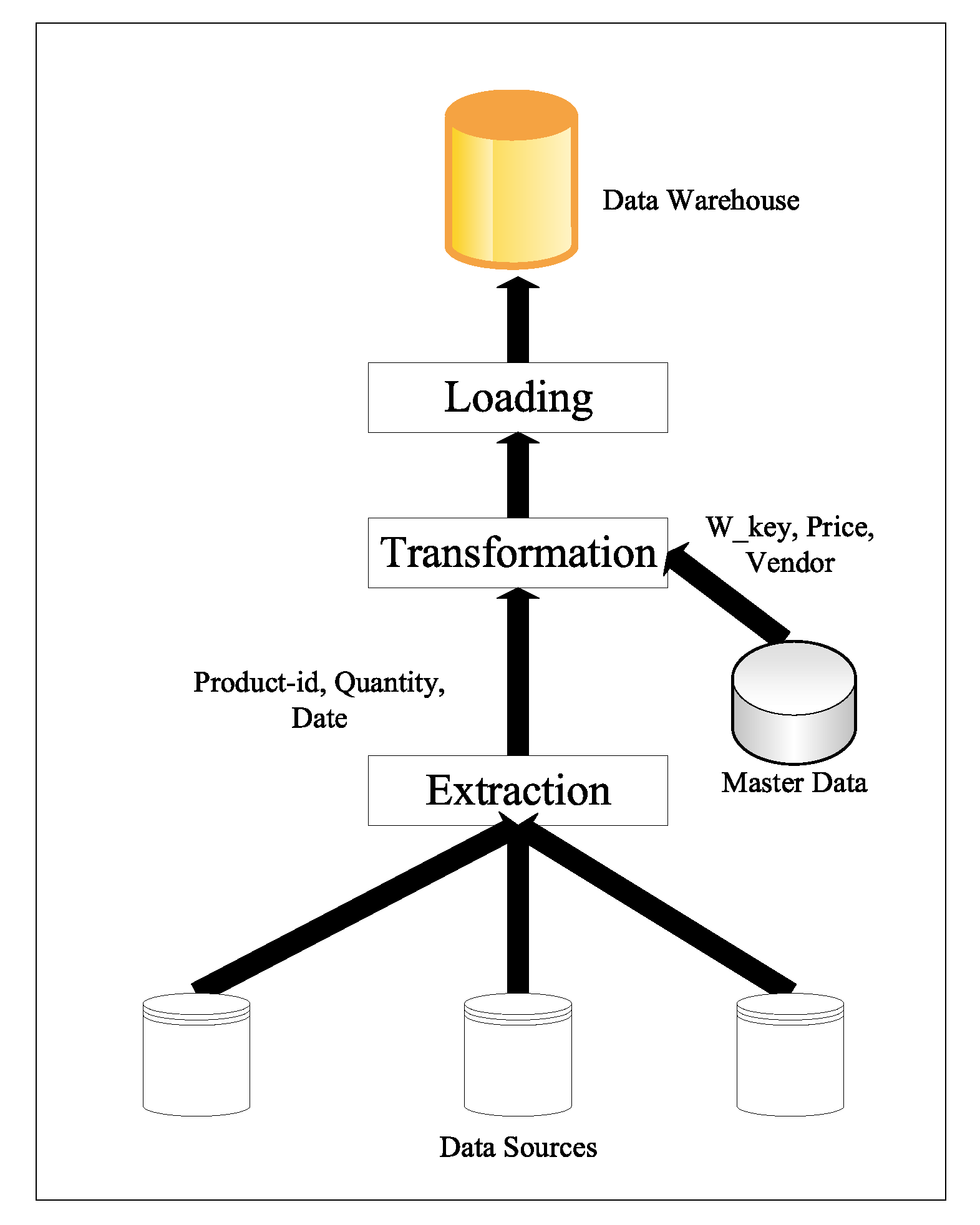
In near-real-time data warehousing typically, joining is performed between primary (unique) key of R input and foreign key of S input. For example, Figure 1 implemented the example of information enrichment. From the figure we consider that attributes product-ID, date, and quantity are extracted from S. In the transformation operation, in addition to key replacement (from source key product-ID to warehouse key W_key) there is some information added, namely, sales price denoted by price to calculate the total amount, and the vendor information denoted by vendor. In the figure the information with attributes’ names W_key, price, and vendor are extracted at runtime from R and are enriched to S using a join operator.
The main problem with the stream-relation join is that the stream input S is fast and bursty in nature, whereas the disk input R is slow due to high I/O cost. Many algorithms have been proposed to implement the join operation between S and R. CACHEJOIN (cache join) is one of them which is considered an optimal algorithm for skew data (non-uniform data). The algorithm consists of two phases, the disk-probing phase and the stream-probing phase. However, these two phases execute sequentially. In this case, the stream input has to unnecessarily wait and therefore the algorithm cannot exploit CPU resources optimally. This ultimately causes the performance of the algorithm to be suboptimal. This is further explained in Section 2.
In this paper we present a robust algorithm called the parallelised cache-based stream relation join (PCSRJ) which enables the execution of both phases of the existing CACHEJOIN algorithm in parallel. This means the disk-probing phase does not wait for finishing the stream-probing phase and vice versa. The new algorithm in this way exploits CPU resources optimally, and that ultimately improves its performance. The further details about the new algorithm are provided in Section 3.
In summary, this paper makes following contributions:
- A well-known stream-relation join algorithm CACHEJOIN has been explored with respect to its limitations.
- A robust algorithm PCSRJ has been introduced in order to improve the performance of CACHEJOIN.
- We propose the cost model for our algorithm, and we validated that cost model.
- We present an experimental analysis of PCSRJ with the existing CACHEJOIN.
The rest of the paper is organised as follows. Section 2 presents a review of existing approaches. Section 3 presents the new algorithm, including its architecture, algorithm, and cost model. Rigorous experimentation on our algorithm is presented in Section 4. Finally, Section 5 concludes the paper.
2. Related Work
In near-real-time (online) data warehousing, we require an efficient stream-relation join that joins the incoming stream tuples with R using low resources in an effective way. In this section we present an overview of various stream-relation joins in detail.
A seminal algorithm MESHJOIN (Mesh Join) [11] has been designed to join R with S. In MESHJOIN, R is divided into partitions. Additionally, S is divided into chunks; the size of each chunk is w. In each iteration the algorithm loads w tuples of S and a partition of R in memory. Every tuple of S is then joined with every partition of R. The algorithm ensures that each tuple from S is joined with the whole of R before it is removed from the join window. Once the whole R gets read, the algorithm restarts its reading. MESHJOIN’s authors report that the algorithm does not perform well with skewed data (frequent tuples). The limitation of MESHJOIN is that when the number of tuples in R changes, the size of disk buffer also changes; that makes memory distribution suboptimal. Therefore, in MESHJOIN, the service rate is inversely proportional to the size of R.
Reduced Mesh Join (R-MESHJOIN) [12] is an extension of MESHJOIN. R-MESHJOIN removes the complexities of MESHJOIN. In that algorithm, performance is improved by allocating optimal memory to the disk buffer and a hash table. Disk buffer is split into variety of logical segments l. In R-MESHJOIN l is greater than one. If l is equal to one then R-MESHJOIN is equal to MESHJOIN. Although in R-MESHJOIN the service improves due to removing unnecessary constraints, the algorithm does not consider common characteristics (skewed distribution) in S.
Partition-based join [13] is an improved version of MESHJOIN. The algorithm finds out the often repeated stream tuples and joins these tuples with a small memory buffer. This is the main distinction between the partition-based join and MESHJOIN. In this algorithm, a wait-buffer is maintained that stores every stream tuple. The disk probe is invoked when wait-buffer is full or the number of stream tuples related to a partition is greater than the threshold. The algorithm ensures that one stream tuple is only joined with a single read from R, which minimises the frequency of disk access. In a partition-based join, there is no limit of waiting time for a stream tuple to be joined. For infrequent stream tuples, the waiting time of a partition-based join is greater than in MESHJOIN.
Semi-stream index join (SSIJ) [14], is an improved version of MESHJOIN. In the SSIJ algorithm, there are three phases—pending, online, and join. In the pending phase, the algorithm fills the input buffer with incoming stream tuples to make a batch. When the input buffer filled, the online phase starts. In the online phase, incoming tuples are ordered based on the frequently used index. The output of tuples is generated immediately if tuples match with the cache. Remaining tuples that are not matched with cache pages of R wait for the last phase—that is, the join phase. When the online phase is complete, the join phase starts, which matches the incoming tuples with the tuples of R that are on the disk. When the join phase is complete, the algorithm again starts the pending phase. The authors of SSIJ reported that there is a worst case when no stream tuple is matched with cache in online phase.
HYBRIDJOIN (Hybrid Join) [15] is combination of index nested loop join (INLJ) [16] and MESHJOIN. HYBRIDJOIN minimises the waiting and processing time of stream tuples by using index on R and deals with stream effectively. However, the algorithm performs suboptimally for non-uniform distributions, which means it is not robust if some tuples from R appear frequently in S.
X-HYBRIDJOIN [17] is a further extension of HYBRIDJOIN that uses indexing on R and caches the most frequent portion of R. In X-HYBRIDJOIN the disk buffer is split into two parts. The first part is non-swappable part that holds frequent pages of R. The second part is the swappable part that one-by-one loads the rest of the partitions of R. Although X-HYBRIDJOIN outperforms HYBRIDJOIN, however, some tuples in the non-swappable part can be infrequent. This does not fully exploit the cache and leaves the room for improving performance.
Optimised X-HYBRIDJOIN [18] is an updated version of X-HYBRIDJOIN. Optimised X-HYBRIDJOIN resolved the problem of unnecessary processing cost by introducing two phases that can work independently. However, the issue of cache suboptimality is still remained.
In [19] the authors defined a new operator for stream-relation join that uses two mechanisms, out-of-order processing and batch processing, in order to increase the service rate. This algorithm splits the fast-arriving stream tuples into miss and hit tuples using two separate threads (batch and out-of-order). In that algorithm, a cache is made that maintains its content by least recently used (LRU) policy. Fast-arriving stream tuples first join with the cache: if a match is found then that tuple is considered as hit tuple and is processed immediately. The tuples that are not matched are known as missed tuples. In that algorithm missed tuples are not processed individually; tuples are processed in the form of batches. Missed tuples are added to the waiting queue; when the waiting queue gets full, key values of all missed tuples are queried to R. The authors of that algorithm reported that when the cache is less useful, then memory allocation between the waiting queue and the cache is suboptimal.
Semi-stream balanced join (SSBJ) [20] deals with many-to-many equijoins efficiently. In SSBJ cache, inequality is used for minimum memory consumption and increase the service rate. There are two phases of SSBJ. First is the cache phase and second is the disk phase. In SSBJ each stream tuple first passes through the cache phase; if a match is found, then output is generated and if a match is not found, then that tuple shifts to the disk phase. In SSBJ, cache size is variable. Cache size is changed based on every join value. This helps to increase the service rate of the SSBJ algorithm.
CACHEJOIN (Cache Join) [21] introduces a cache module that stores frequent tuples of R and joins these with S. CACHEJOIN has two phases; one is the stream-probing phase, and the other is the disk-probing phase. The stream-probing phase deals with only a limited portion of R. A big part of R is dealt with by the disk-probing phase. For every tuple that comes from the stream, it first passes through the stream-probing phase to find a quick match. If a match is found, that tuple is generated in the output; otherwise that tuple goes to the disk-probing phase. After that disk-probing phase, the algorithm again switches back to the stream-probing phase. However, in CACHEJOIN, due to sequential execution of both phases, stream tuples unnecessarily wait to complete the join, which decreases the performance of the algorithm. The performance can be improved if the two phases can execute in parallel which has not been considered in CACHEJOIN.
3. Parallelisation of CACHEJOIN
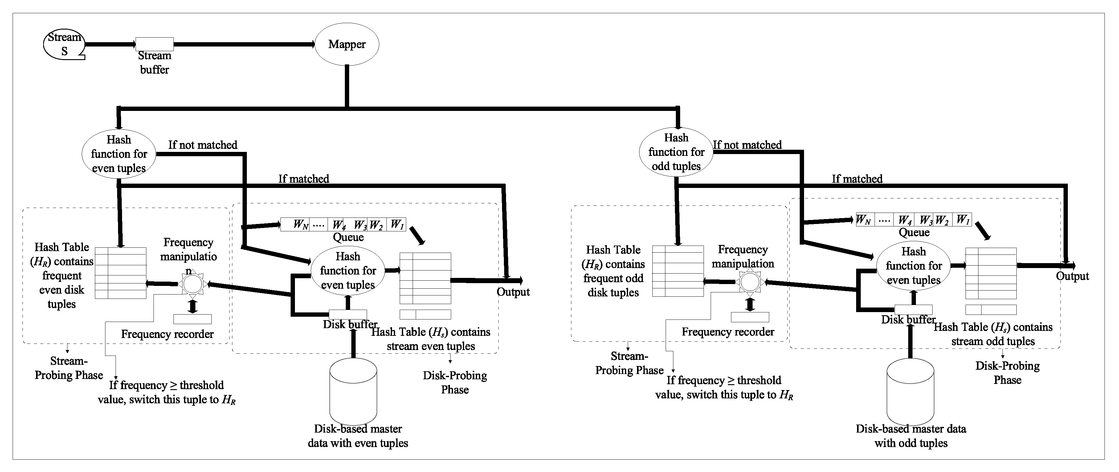
In this section, we present a robust algorithm called the parallelised cache-based stream relation join (PCSRJ). The algorithm distributes R at two different computer nodes using hash partitioning strategy. The hash function is based on even and odd values of a join attribute, e.g., productid in R. Additionally, an index has been applied at R using the same join attribute. At each node the algorithm implements both phases of the CACHEJOIN algorithm. The incoming stream tuples are directed towards the relevant node based on even and odd values of its join attribute using a mapper. The mapper implements the same hash function that we used for partitioning R. The following subsections present the architecture, algorithm, and cost model of PCSRJ.
3.1. Architecture
The major components of PCSRJ at each node are: a cache H for caching frequent tuples of R, a queue Q that stores join attribute values, a hash table H that stores the stream tuples that are not matched in the stream-probing phase, and a disk buffer that stores a partition of R. Three other minor components are the mapper, stream buffer, and frequency recorder. The mapper is used to distribute the incoming stream tuples to the each node, and the stream buffer is used to hold the stream tuples for a short interval while the tuple in memory gets processed. The frequency recorder is used to find the frequent tuples of R in S and is responsible for loading them to H. The memory taken up by these three components is very little so we do not include that in our memory cost calculation. However, to show their working we include these components in the architecture. The execution architecture of PCSRJ is shown in Figure 2.
At each node PCSRJ consists of a stream-probing (also called cache) phase and a disk-probing phase. Every new stream tuple arrives from the mapper and the node is first directed to the stream-probing phase. If the tuple matches with corresponding tuple in the stream-probing phase, the output is generated; otherwise it is directed to the disk-probing phase where it is stored in H and its join attribute value is stored in Q. The algorithm then loads a partition of R into the disk buffer using the most old join attribute value from Q as an index. After loading a partition of R, the algorithm looks at each tuple from the disk buffer H. If the matched tuple is found in H, the algorithm processes that tuple in the output and removes it from H along with its join attribute value from Q. Once the algorithm matches all the tuples from the disk buffer, the algorithm switches back to the stream-probing phase. By using parallel execution of the join at two different nodes, our experiment showed that the number of tuples joined per second significantly increased as compared to existing CACHEJOIN.
3.2. Algorithm
The pseudo-code for PCSRJ is presented in Algorithm 1. Since the identical threads of the PCSRJ algorithm run at both nodes, we present the pseudo-code for one node. Line 1 in the algorithm represents an infinite execution of the algorithm. This is the norm in such types of stream-based algorithms. For each incoming stream tuple, the algorithm maps it to the relevant node by applying the hash function on the join attribute value (line 2).
Lines 3 to 10 specify the stream-probing phase for either of the two nodes. In line 3, the algorithm reads w stream tuples from the stream buffer and one-by-one matches each stream tuple t from w into H. If the matching tuple is found from H, the algorithm generates tuple t as an output (lines 4 to 6). If the matching tuple is not found, the algorithm then loads t into H and enqueues its join attribute value to Q (lines 7 to 10). In the first iteration, since hash table is empty, the value of w is equal to the size of in terms of tuples. Meanwhile, from the second iteration and onward, the value of w depends on the number of slots that are emptied from in the previous iteration.
Lines 11 to 21 specify the disk-probing phase where the algorithm processes the stream tuples which are not matched in the stream-probing phase. In line 11 the algorithm loads b number of tuples from R into the disk buffer. The algorithm then reads each tuple r from the disk buffer one-by-one and looks for matching tuple into H. If the matched tuple is found, the algorithm generates output for tuple r (lines 12 to 14). Since the join type is one-too-many, there can be more matches against r. The total number of matches is stored in f (line 15). Lines 16 to 18 determine whether tuple r is frequent. Therefore, the value of f is compared with the preset frequency threshold. If f is greater than the frequency threshold, the algorithm loads tuple r to H. If H is full, the algorithm overwrites a least frequent tuple in H by r. Finally, the algorithm removes the matched tuples against r from H along with their join attribute values from Q (line 19). The algorithm also enables the tuning of the threshold value based on the following principle. If tuples are removed from the cache frequently, then there is need to increase the value of the threshold. Similarly, if the cache is not getting full even after a complete round of R then threshold is too high and should be lowered down slightly.
| Algorithm 1 PCSRJ algorithm for one node. |
| Input: Stream S and a master data relation R with index on the join attribute. Output: Parameters: w (Where w = w + w) tuples of S, b number of tuples of R
|
3.3. Cost Model
This section presents the cost model for our PCSRJ. The cost model is similar in nature to the CACHEJOIN [21] cost model which consists of both memory and processing costs. Equation (1) shows the memory cost for PCSRJ. As mentioned above, the components stream buffer, mapper, and frequency recorder are tiny (0.05 MB was enough for all our experiments), and therefore, we do not include these in our memory cost calculation. Equation (2) explains the processing cost for PCSRJ. Symbols used in both cost calculations are presented in Table 1.
3.3.1. Memory Cost
The major components to which memory is assigned are two hash tables H and H, the disk buffer, and the queue Q. We calculate double memory for each components as the PCSRJ algorithm runs in two computer nodes. To make it simple, we first calculate the memory for each component separately and then sum-up the individual memory requirements to calculate the total. Therefore, memory taken up by each component at both nodes is calculated as follows:
- Memory for the disk buffer in bytes =
- Memory for H in bytes =
- Memory for H in bytes =
- Memory for Q in bytes =
By combining the above, the total memory for PCSRJ can be calculated as shown in Equation (1).
3.3.2. Processing Cost
In this section we compute the processing cost for PCSRJ algorithm. Similarly to the memory, we calculate double the processing cost for each component due to running the two algorithm threads in parallel on two nodes. Again, we first compute cost for each component separately and then add-up all these costs to compute the total cost for one loop iteration.
- Cost of reading b number of tuples from R to the disk buffer =
- Cost of matching w tuples in H =
- Cost of matching all tuples in the disk buffer to H =
- Cost of matching the frequency of all tuples in the disk buffer with the threshold value =
- Cost to produce output for w tuples =
- Cost to produce output for w tuples =
- Cost to read w tuples from the stream buffer =
- Cost to read w tuples from the stream buffer =
- Cost to append w tuples into H and Q =
- Cost to delete w tuples from H and Q =
The total processing cost for one loop iteration can be computed by combining the above individual processing costs, as shown in Equation (2).
In the above equation is used to convert nanoseconds into seconds. In each iteration, since the algorithm processes w and w tuples of S at one node, the total number of tuples process in one second (also know as service rate ) can be computed using Equation (3).
4. Experimental Work
We conducted a rigorous experimental study for our algorithm. Before presenting our results, we first describe the experimental setup, including the hardware and datasets we used in our experiments.
4.1. Hardware Specification
We used a Core-i7 computer with 8 GB ram and a 1 TB hard drive. We implemented the both algorithms in Java using its integrated development environment (IDE) Eclipse. For processing cost in terms of time measurements, we used builtin function from Java API called nanoTime(). The master data R were stored on the disk using the MySQL 5.7 database.
4.2. Data Specification
A Zipfian distribution of the foreign keys in the stream data matches distributions that are observed in a wide range of applications [22]. We therefore created a data generator that can produce such a Zipfian distribution. A Zipfian distribution is parameterized by the exponent of the underlying Zipf’s Law [23]. The same distribution was used in evaluating original CACHEJOIN. We used size of R from 1 million to 8 million tuples. The size of every tuple in R was 120 bytes and size of every tuple in stream was 20 bytes. The size of each node in Q was 12 bytes. Same sizes of disk tuple, stream tuple, and Q node were used in CACHEJOIN. For each measurement, we calculated the 95% confidence interval of the mean based on at least 1000 runs for one setting. The detailed data specifications that we used in our experiments are shown in Table 2.
4.3. Performance Evaluation
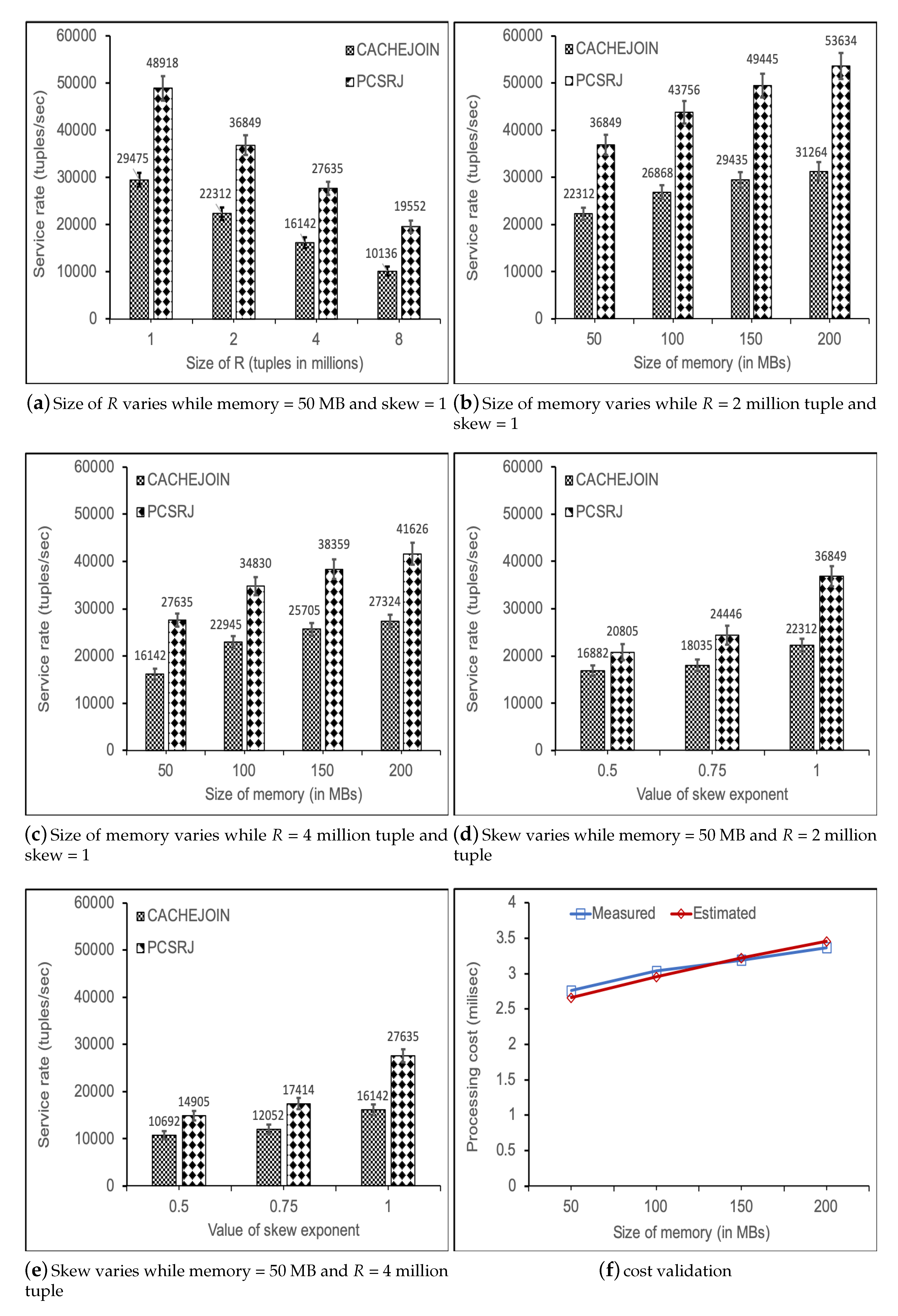
We evaluated the performance (service rate) of PCSRJ by comparing it to CACHEJOIN. We compared the service rate with respect to three external parameters, namely, available memory for the algorithm, size of R, and level of skew in the stream data.
4.3.1. Service Rate Analysis by Varying R
In our first experiment we evaluated the service rate of PCSRJ with CACHEJOIN by varying the size of R from 1 million tuples to 8 million tuples. We fixed the other two parameters: memory size was equal to 50 MB and the level of skew in the stream data was equal to 1. The results of our experiment are shown in Figure 3a. From the figure it can be seen that PCSRJ performed ≈ two times better than CACHEJOIN for = 8 million tuples and ≈1.65 times better for = 1 million tuples.
4.3.2. Service Rate Analysis by Varying Memory
In this experiment we evaluated the service rates of both algorithms by varying the size of memory available for the algorithms. We varied the size of available memory for two different settings of R, i.e., 2 million tuples and 4 million tuples. We fixed the level of skew in the stream data to be equal to 1. The results of both experiments are shown in Figure 3b,c. From Figure 3b we observed that PCSRJ was ≈1.65 times faster than CACHEJOIN with very limited memory (50 MB) and ≈1.71 times faster for 200 MB. Similar behaviour can can be observed in Figure 3c. This shows that the gain in the service rate was due to parrallelisation of the existing algorithm.
4.3.3. Service Rate Analysis by Varying Skew
In this experiment we evaluated the service rates of both algorithms by varying the level of skew in the stream data. We varied the value of skew between 0 and 1. At the skew value of 0 the stream was fully uniform, and at the skew value of 1 the stream was skewed (non-uniform). Again we tested the skew for two different settings of R, i.e., 2 million tuples and 4 million tuples. We kept the size of available memory fixed to 50 MB. The results of both experiments are shown in Figure 3d,e. It is clear from the both figures that PCSRJ started performing better as soon as the skew appeared in the stream data, and this improvement became more evident and visible as the value of skew increased. For the high values of skew (i.e., equal to 1) PCSRJ performed ≈1.65 times better than CACHEJOIN. Although CACHEJOIN also exploits the feature of skew in the stream data, due to non parallelisation the algorithm can not perform maximally. We did not evaluate the performance for skew values higher than 1, as the higher skew values would imply comparatively short tails. However, we presume that the improvement in the service rate will continue for such short tails.
4.3.4. Cost Validation
Finally, we validated the cost models for the PCSRJ algorithms; we compared the calculated cost for a central cost parameter, , with measurements of . Figure 3f depicts the results of the experiment. From the figure it is clear that the calculated cost is very close to the measured cost. This is a proof for the correctness of our implementation for the PCSRJ algorithms.
5. Conclusions
Minimising latency in processing streaming data is a primary objective of stream-relation joins. Contributing to this, in the paper we presented a robust algorithm called PCSRJ (parallelised cache-based stream relation join). PCSRJ extends the existing CACHEJOIN algorithm by distributing the disk-based master data (relation R) on multiple nodes and parallelising the algorithm by implementing the concept of multi-threading in it. This feature of parallelisation enables the algorithm to exploit the use of CPU resources optimally. We proposed the design, implementation, and cost model for our algorithm. Our experimental study showed that PCSRJ significantly outperformed CACHEJOIN for all three external parameters, i.e., available memory, size of R, and level of skew in the stream data. We also validated our cost model by comparing it with the empirical cost which verified the correct implementation of PCSRJ. We have plans to extend our PCSRJ for joining streaming data with multiple tables in the master data. Another direction for our future work is to implement the algorithm on several nodes, e.g., a cluster of computers.
Author Contributions
M.A.N. conceptualized the idea and formulated the research goals and aims. H.U.K. administrated the project and coordinated responsibility for the research activities planning and execution. S.A. developed the methodology and implemented the design of the research. N.J. reviewed and polished the draft of the paper. All authors have read and agreed to the published version of the manuscript.
Funding
This research received no external funding.
Acknowledgments
The research is technically supported by National University of Computer & Emerging Sciences, Pakistan and Auckland University of Technology, Auckland, New Zealand while it is financially supported by Qatar University, Qatar.
Conflicts of Interest
The authors declare no conflict of interest.
References
- Martínez, A.B.; Galvis-Lista, E.A.; Florez, L.C.G. Modeling techniques for extraction transformation and load processes: A critical review. In Proceedings of the 6th Euro American Conference on Telematics and Information Systems, Valencia, Spain, 23–25 May 2012; pp. 41–47. [Google Scholar]
- Wijaya, R.; Pudjoatmodjo, B. An overview and implementation of extraction-transformation-loading (ETL) process in data warehouse (Case study: Department of agriculture). In Proceedings of the 2015 3rd International Conference on Information and Communication Technology (ICoICT), Bali, Indonesia, 27–29 May 2015; pp. 70–74. [Google Scholar]
- Arasu, A.; Cherniack, M.; Galvez, E.; Maier, D.; Maskey, A.S.; Ryvkina, E.; Stonebraker, M.; Tibbetts, R. Linear road: A stream data management benchmark. In Proceedings of the Thirtieth International Conference on Very large Data Bases, Toronto, ON, Canada, 31 August–3 September 2004; Volume 30, pp. 480–491. [Google Scholar]
- Cranor, C.; Gao, Y.; Johnson, T.; Shkapenyuk, V.; Spatscheck, O. Gigascope: High performance network monitoring with an SQL interface. In Proceedings of the 2002 ACM SIGMOD International Conference on Management of Data, Madison, WI, USA, 4–6 June 2002; p. 623. [Google Scholar]
- Bonnet, P.; Gehrke, J.; Seshadri, P. Towards sensor database systems. In Proceedings of the International Conference on mobile Data management, Hong Kong, China, 8–10 January 2001; pp. 3–14. [Google Scholar]
- Cortes, C.; Fisher, K.; Pregibon, D.; Rogers, A. Hancock: A language for extracting signatures from data streams. In Proceedings of the Sixth ACM SIGKDD International Conference on Knowledge Discovery and Data Mining, Boston, MA, USA, 23–27 August 2000; pp. 9–17. [Google Scholar]
- Gilbert, A.C.; Kotidis, Y.; Muthukrishnan, S.; Strauss, M. Surfing wavelets on streams: One-pass summaries for approximate aggregate queries. In Proceedings of the 27th VLDB Conference, Roma, Italy, 11–14 September 2001; Volume 1, pp. 79–88. [Google Scholar]
- Arasu, A.; Babu, S.; Widom, J. An Abstract Semantics and Concrete Language for Continuous Queries over Streams and Relations. Available online: http://ilpubs.stanford.edu:8090/563/1/2002-57.pdf (accessed on 7 August 2020).
- Franklin, M.J.; Jeffery, S.R.; Krishnamurthy, S.; Reiss, F.; Rizvi, S.; Wu, E.; Cooper, O.; Edakkunni, A.; Hong, W. Design Considerations for High Fan-In Systems: The HiFi Approach. In Proceedings of the CIDR 2005, Asilomar, CA, USA, 4–7 January 2005; Volume 5, pp. 24–27. [Google Scholar]
- Gonzalez, H.; Han, J.; Li, X.; Klabjan, D. Warehousing and analyzing massive RFID data sets. In Proceedings of the 22nd International Conference on Data Engineering (ICDE’06), Atlanta, GA, USA, 3–7 April 2006; p. 83. [Google Scholar]
- Polyzotis, N.; Skiadopoulos, S.; Vassiliadis, P.; Simitsis, A.; Frantzell, N. Meshing streaming updates with persistent data in an active data warehouse. IEEE Trans. Knowl. Data Eng. 2008, 20, 976–991. [Google Scholar] [CrossRef]
- Naeem, M.A.; Dobbie, G.; Weber, G.; Alam, S. R-MESHJOIN for near-real-time data warehousing. In Proceedings of the ACM 13th international workshop on Data warehousing and OLAP, Toronto, ON, Canada, 30 October 2010; pp. 53–60. [Google Scholar]
- Chakraborty, A.; Singh, A. A partition-based approach to support streaming updates over persistent data in an active datawarehouse. In Proceedings of the 2009 IEEE International Symposium on Parallel & Distributed, Rome, Italy, 23–29 May 2009; pp. 1–11. [Google Scholar]
- Bornea, M.A.; Deligiannakis, A.; Kotidis, Y.; Vassalos, V. Semi-streamed index join for near-real time execution of ETL transformations. In Proceedings of the 2011 IEEE 27th International Conference on Data Engineering, Hannover, Germany, 11–16 April 2011; pp. 159–170. [Google Scholar]
- Naeem, M.A.; Dobbie, G.; Weber, G. HYBRIDJOIN for near-real-time data warehousing. Int. J. Data Warehous. Min. (IJDWM) 2011, 7, 21–42. [Google Scholar] [CrossRef] [Green Version]
- Ramakrishnan, R.; Gehrke, J. Database Management Systems; McGraw Hill: New York, NY, USA, 2000. [Google Scholar]
- Naeem, M.A.; Dobbie, G.; Weber, G. X-HYBRIDJOIN for near-real-time data warehousing. In Proceedings of the British National Conference on Databases, Manchester, UK, 12–14 July 2011; pp. 33–47. [Google Scholar]
- Naeem, M.; Dobbie, G.; Weber, G. Optimised X-HYBRIDJOIN for near-real-time data warehousing. In Proceedings of the Twenty-Third Australasian Database Conference (ADC), Melbourne, Australia, 31 January–3 February 2012. [Google Scholar]
- Derakhshan, R.; Sattar, A.; Stantic, B. A new operator for efficient stream-relation join processing in data streaming engines. In Proceedings of the 22nd ACM International Conference on Information & Knowledge Management, San Francisco, CA, USA, 27 October–1 November 2013; pp. 793–798. [Google Scholar]
- Naeem, M.A.; Weber, G.; Lutteroth, C. A memory-optimal many-to-many semi-stream join. Distrib. Parallel Databases 2019, 37, 623–649. [Google Scholar] [CrossRef]
- Naeem, M.A.; Bajwa, I.S.; Jamil, N. A Cached-Based Stream-Relation Join Operator for Semi-Stream Data Processing. Int. J. Data Warehous. Min. (IJDWM) 2016, 12, 14–31. [Google Scholar] [CrossRef]
- Anderson, C. The Long Tail: Why the Future of Business Is Selling Less of More; Academy of Management: Briarcliff Manor, NY, USA, 2006. [Google Scholar]
- Knuth, D.E. The Art of Computer Programming, Volume 3: Sorting and Searching, 2nd ed.; Addison Wesley Longman Publishing Co., Inc.: Redwood City, CA, USA, 1998; pp. 400–401. [Google Scholar]
Figure 1.
An example of stream-relation join during the transformation phase.

Figure 2.
Execution architecture of PCSRJ.

Figure 3.
Performance evaluation.


Table 1.
Symbols used in memory and processing cost calculation of PCSRJ.
| Parameter Name | Notation |
|---|---|
| Size of the disk tuple (bytes) | V |
| Size of the disk buffer (tuples) | b |
| Number of stream tuples processed in every iteration through H | w |
| Number of stream tuples processed in every iteration through H | w |
| Size of H in tuples | h |
| Memory weight for H | |
| Memory weight for Q | 1 − |
| Cost of matching one tuple to the either hash tables (nano seconds) | c |
| Cost of producing one tuple in the output (nano seconds) | c |
| Cost of deleting one tuple from the either hash tables and Q (nano seconds) | c |
| Cost of reading one stream tuple from the stream buffer (nano seconds) | c |
| Cost of loading one tuple in the either hash tables and Q (nano seconds) | c |
| Cost of match the frequency of one disk tuple with the specific threshold value (nano seconds) | c |
| Cost to denote for one loop iteration (seconds) | c |
Table 2.
Synthetic dataset specifications.
| Parameter | Value |
|---|---|
| Memory used by the algorithm | 50 MB to 200 MB |
| Size of R | 8 million tuples |
| Disk tuple size | 120 bytes |
| Stream size | infinite |
| Stream tuple size | 20 bytes |
| Size of each node in the queue | 12 bytes |
| Stream data | based on Zipf’s law [23] (skew value from 0 to 1) |
© 2020 by the authors. Licensee MDPI, Basel, Switzerland. This article is an open access article distributed under the terms and conditions of the Creative Commons Attribution (CC BY) license (http://creativecommons.org/licenses/by/4.0/).
Share and Cite
MDPI and ACS Style
Naeem, M.A.; Khan, H.U.; Aslam, S.; Jamil, N. Parallelisation of a Cache-Based Stream-Relation Join for a Near-Real-Time Data Warehouse. Electronics 2020, 9, 1299. https://doi.org/10.3390/electronics9081299
AMA Style
Naeem MA, Khan HU, Aslam S, Jamil N. Parallelisation of a Cache-Based Stream-Relation Join for a Near-Real-Time Data Warehouse. Electronics. 2020; 9(8):1299. https://doi.org/10.3390/electronics9081299
Chicago/Turabian StyleNaeem, M. Asif, Habib Ullah Khan, Saad Aslam, and Noreen Jamil. 2020. "Parallelisation of a Cache-Based Stream-Relation Join for a Near-Real-Time Data Warehouse" Electronics 9, no. 8: 1299. https://doi.org/10.3390/electronics9081299
Note that from the first issue of 2016, this journal uses article numbers instead of page numbers. See further details here.