Vibration Analysis of Piezoelectric Cantilever Beams with Bimodular Functionally-Graded Properties

Abstract

Piezoelectric materials have been found to have many electromechanical applications in intelligent devices, generally in the form of the flexible cantilever element; thus, the analysis to the corresponding cantilever is of importance, especially when advanced mechanical properties of piezoelectric materials should be taken into account. In this study, the vibration problem of a piezoelectric cantilever beam with bimodular functionally-graded properties is solved via analytical and numerical methods. First, based on the equivalent modulus of elasticity, the analytical solution for vibration of the cantilever beam is easily derived. By the simplified mechanical model based on subarea in tension and compression, as well as on the layer-wise theory, the bimodular functionally-graded materials are numerically simulated; thus, the numerical solution of the problem studied is obtained. The comparison between the theoretical solution and numerical study is carried out, showing that the result is reliable. This study shows that the bimodular functionally-graded properties may change, to some extent, the dynamic response of the piezoelectric cantilever beam; however, the influence could be relatively small and unobvious.

1. Introduction

The piezoelectric effect is among the most exploited transduction mechanisms for multiscale electromechanical applications, such as sensors, actuators and energy conversion devices, in which piezoelectric vibrational energy harvesting is attractive. For piezoelectric materials, there is a wide spectrum, from piezoelectric ceramics, perovskite structured lead zirconate titanate (PZT), to piezoelectric polymer films, polyvinylidene fluoride (PVDF). Among the piezoelectric materials, piezoelectric ceramics (PZT) is currently regarded as the most promising material system of piezoelectric vibrational energy harvesting devices since it can produce large output power, effective electromechanical coupling and high mechanical strain under an applied electric field [1,2]. Usually, piezoelectric sensors are a laminated original made of ceramic slice; thus, it is easy to result in stress concentration and also to develop interfacial microcracks. For overcoming this difficulty, functionally-graded piezoelectric materials (FGPM), whose properties of materials continuously change along certain direction, are developed. In FGPM, the obvious interface is disappeared, thus effectively avoiding the damage caused by the stress concentration at the interface. Studies concerning FGPM and corresponding structures made of FGPM have attracted the interests of scholars from all over the world [3,4,5,6,7,8].

In the existing works, the vibration problems of piezoelectric structures with functionally-graded properties have been extensively studied, and some valuable results were obtained. Based on the first-order shear theory, Mahinzare et al. [9] studied the free vibration of a rotating circular nanoplate composed of two directional functionally-graded piezo materials (two directional FGPM). The steady-state forced vibration of functionally-graded piezoelectric beams was investigated by Yao and Shi [10]. Shakeri and Mirzaeifar [11] made static and dynamic analysis of thick functionally-graded plates with piezoelectric layers based on the layerwise finite element model. Ebrahimi [12] investigated, analytically, the vibrations and dynamic response of functionally-graded plate, which is integrated with piezoelectric layers in thermal environment. Using a numerical method, Chen et al. [13] investigated the transient response and natural vibration of FGPM curved beam. Li et al. [14] studied the free vibration of FGM beams with surface-bonded piezoelectric layers, which is statically thermal post-buckled and subjected to both voltage and temperature rise. Huang and Shen [15] investigated the dynamic response and vibration of FGM plates with piezoelectric actuators in thermal environments. Fu et al. [16] made a nonlinear analysis of free vibration, dynamic stability and buckling for the FGPM beams in thermal environment. Li and Shi [17] studied the free vibration of a FGPM beam by using state-space based differential quadrature. Considering that there have been many studies in this field, it is not necessary to review them in detail here.

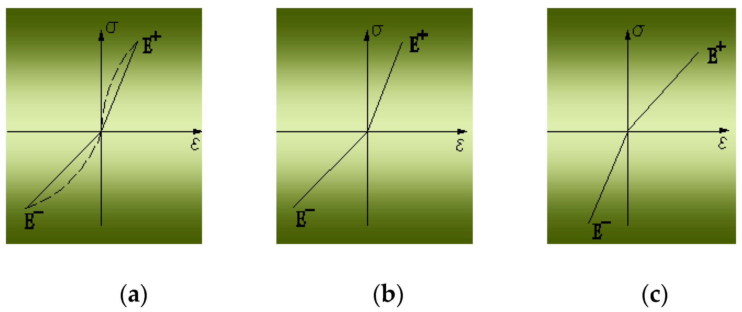
Compared with the FGPM, the bimodular effect of materials is relatively less known. However, many investigations have indicated that some materials [18,19], such as graphite, plastics, ceramics, concrete, steel, polymeric materials, powder metallurgy materials and some composites, will perform different elastic properties when they are in tension and compression; that is, they have different moduli when tensioned and compressed and thus are named bimodular materials [20] (see Figure 1), in which $\sigma$ is the stress, $\epsilon$ is the strain and $E^{+}$ and $E^{-}$ represents the tensile modulus of elasticity and compressive one, respectively. In 1982, the Elasticity Theory of Different Moduli, by Ambartsumyan [21], was published, in which the constitutive model for bimodular materials and the corresponding application in structural analysis were introduced systematically. The publication of this book marks that the idea of bimodular materials entered the field of vision of scholars from all over the world. Thereafter, bimodular problems for materials and structures have been investigated extensively [22,23,24,25]. These works indicated that the bimodular effect of materials will modify, to some extent, the mechanical behaviors of structures. Unfortunately, due to the complexity in analysis, the bimodular effect of materials is often neglected. Although some works have been carried out to combine the functionally-graded properties with bimodular effect of materials, for example, [26], the existing works appear insufficient. In fact, not only pure functionally-graded materials but also functionally-graded piezoelectric materials may have a certain degree of bimodular effect. Simple neglect will inevitably lead to analytical errors, which could further influence the design application of the electromechanical devices based on piezoelectric effect.

He et al. [27] considered the bimodular effect during the analysis of functionally-graded piezoelectric materials and structures for the first time, and presented a two-dimensional analytical solution for a FGPM bimodular cantilever beam. Thereafter, aiming at the static problem of a bimodular FGPM cantilever, He et al. [28] neglected some unimportant factors to derive the one-dimensional theoretical solution and, based on the model of tension-compression subarea, conducted a two-dimensional numerical simulation. However, the existing works appear insufficient since there is no dynamic solution to the corresponding problem. At present, for a cantilever-type structure which is extensively adopted in piezoelectric sensors devices, the bimodular functionally-graded effect on its vibration has not been investigated. In addition, for piezoelectric polymer elements, the vibration problem, due to flexible and lightweight characters of the elements, is particularly acute, which also deserves further research.

In this paper, the free damping vibration problem of a piezoelectric cantilever beam with bimodular functionally-graded properties is analyzed by using analytical and numerical methods. The paper is organized as follows: In Section 2, the problem studied is briefly described and the constitutive relation for bimodular functionally-graded piezoelectric materials is presented. In Section 3, we derive the equivalent modulus of elasticity and obtain the analytical solution of the problem described. The numerical simulation for the problem is performed step by step in Section 4 and the corresponding comparisons and discussions are given in Section 5. Based on the results obtained in this study, some main conclusions are presented in Section 6.

2. The Problem Description

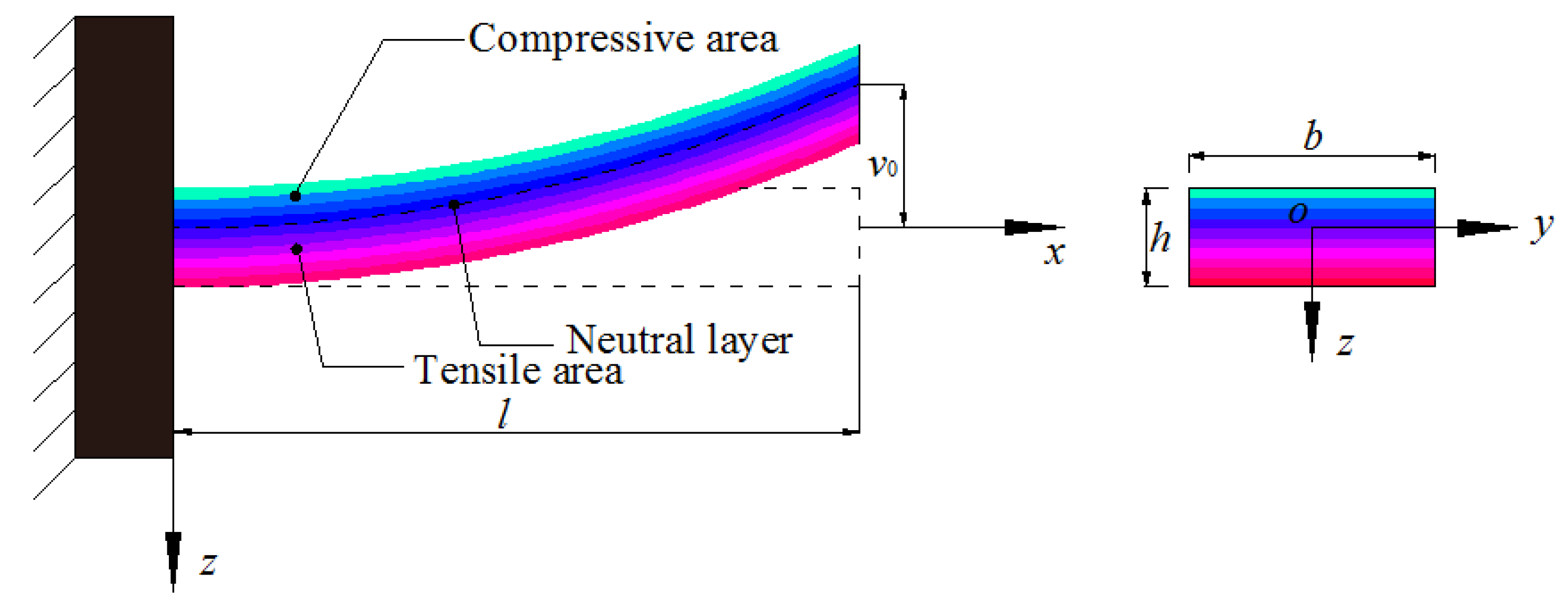
An FGPM orthotropic cantilever beam with different tensile and compressive properties is considered here, and the corresponding Cartesian coordinates system $(x,y,z)$ is established, as depicted in Figure 2, where the right end of the beam is free and the left end is fully fixed; $h$ is the rectangular section height of the beam, $b$ is the section width and $l$ is the beam length ($h<<l$). By exerting a concentrated load at the right end of the beam, an initial displacement $v_0$ is generated at this end of the beam, as depicted in Figure 2. Then, by removing the load suddenly, the beam will freely vibrate until it ceases due to the existence of damping.

During the bending vibration, the beam will continuously present downward bending and upwards bending up to the last cease. In the downward (or upward) bending, the tensile and compressive areas, bound by the neutral layer, will take turns to generate; this physical phenomenon is different from the corresponding static problem, which has an unchanged tensile area and compressive area [27,28]. Therefore, unlike a bending beam in static analysis, in the vibration problem here, it seems that there is no definite tensile or compressive area in the beam. For the convenience of the following analysis, however, we assume in this study that the tensile or compressive area is defined in the present of initial displacement, i.e., the upper part of the beam is in compression and the lower part is in tension, as shown in Figure 2.

Note that the physical parameters of materials of the beam are also functions of coordinates due to the functionally-graded property. In present study, we assume physical parameters vary only along the thickness direction. Thus, all the material parameters are assumed to change with z, according to the following relations.

$$\begin{array}{l}{s}_{ij}^{+}=s_{ij}^0{F}^{+}(z),d_{ij}^{+}=d_{ij}^0{F}^{+}(z),{\lambda }_{ij}^{+}={\lambda }_{ij}^0{F}^{+}(z),\\ s_{ij}^{-}=s_{ij}^0{F}^{-}(z),d_{ij}^{-}=d_{ij}^0{F}^{-}(z),{\lambda }_{ij}^{-}={\lambda }_{ij}^0{F}^{-}(z)\end{array},$$

(1)

in which, $F^{+}(z)=e^{{\alpha }_{1}z/h},F^{-}(z)=e^{{\alpha }_{2}z/h}$ are the tensile and compressive gradient functions, respectively; superscript “+” represents tension and “−” compression; $d_{ij}^{+/-},{\lambda }_{ij}^{+/-},s_{ij}^{+/-}$ are piezoelectric coefficient, dielectric coefficient and elastic coefficient, respectively; $d_{ij}^0,{\lambda }_{ij}^0,s_{ij}^0$ are values at the neutral layer of the corresponding material parameters. It should be noted here that the neutral layer is defined at $z=0$, whose determination has been reported in our previous study on static problem [27,28]. The proposal of the neutral layer stems from the static problem but is still adopted in dynamic counterpart; otherwise, the so-called subarea in tension and compression cannot be realized. Furthermore, note that a set of very small electrodes are adhered discontinuously to the lower and upper surfaces of the beam and the beam is then poled along the direction of z.

Suppose that, in a two-dimensional problem, the stress and strain components is denoted by ${\sigma }_x^{+/-},{\sigma }_z^{+/-},{\tau }_{zx}^{+/-}$ and ${\epsilon }_x^{+/-},{\epsilon }_z^{+/-},{\gamma }_{zx}^{+/-}$, respectively; the electrical displacement and the electrical field components by $D_x^{+/-},D_z^{+/-}$ and $E_x^{+/-},E_z^{+/-}$, respectively. Therefore, the physical equations are

$$\left\{\begin{array}{l}{\epsilon }_x^{+/-}\\ {\epsilon }_z^{+/-}\\ {\gamma }_{zx}^{+/-}\end{array}\right\}=\left[\begin{array}{ccc}{s}_{11}^{+/-}& s_{13}^{+/-}& 0\\ s_{13}^{+/-}& s_{33}^{+/-}& 0\\ 0& 0& s_{44}^{+/-}\end{array}\right]\left\{\begin{array}{l}{\sigma }_x^{+/-}\\ {\sigma }_z^{+/-}\\ {\tau }_{zx}^{+/-}\end{array}\right\}+\left[\begin{array}{ll}0& d_{31}^{+/-}\\ 0& d_{33}^{+/-}\\ d_{15}^{+/-}& 0\end{array}\right]\left\{\begin{array}{l}{E}_x^{+/-}\\ E_z^{+/-}\end{array}\right\}$$

(2)

and

$$\left\{\begin{array}{l}{D}_x^{+/-}\\ D_z^{+/-}\end{array}\right\}=\left[\begin{array}{lll}0& 0& d_{15}^{+/-}\\ d_{31}^{+/-}& d_{33}^{+/-}& 0\end{array}\right]\left\{\begin{array}{l}{\sigma }_x^{+/-}\\ {\sigma }_z^{+/-}\\ {\tau }_{zx}^{+/-}\end{array}\right\}+\left[\begin{array}{cc}{\lambda }_{11}^{+/-}& 0\\ 0& {\lambda }_{33}^{+/-}\end{array}\right]\left\{\begin{array}{l}{E}_x^{+/-}\\ E_z^{+/-}\end{array}\right\},$$

(3)

in which superscript “+/−” denotes “tension/compression”, similar to Equation (1). Until now, Equations (1)–(3) construct the materials relation considering piezoelectric effect as well as bimodular functionally-graded properties.

3. Equivalent Modulus of Elasticity and Analytical Solution

For a relatively shallow beam, the stress and strain along x direction, ${\sigma }_x^{+/-}$ and ${\epsilon }_x^{+/-}$, are dominant, while other stresses and strains along z direction, ${\sigma }_z^{+/-}$ and ${\tau }_{zx}^{+/-}$ as well as ${\epsilon }_z^{+/-}$ and ${\gamma }_{zx}^{+/-}$, are less important. Thus, the constitutive relation of FGPM with bimodular effect, that is, Equations (2) and (3), may be further simplified as,

$$\{\begin{array}{l}{\epsilon }_x^{+/-}=s_{11}^{+/-}{\sigma }_x^{+/-}+d_{31}^{+/-}{E}_z^{+/-}\\ {\epsilon }_z^{+/-}=0\\ {\gamma }_{zx}^{+/-}=0\end{array}$$

(4)

and

$$\{\begin{array}{l}{D}_x^{+/-}={\lambda }_{11}^{+/-}{E}_x^{+/-}\\ D_z^{+/-}=d_{31}^{+/-}{\sigma }_x^{+/-}+{\lambda }_{33}^{+/-}{E}_z^{+/-}\end{array}.$$

(5)

In existing studies for the two-dimensional problem [27,29], $D_x>>D_z$ may be found; thus, it may be assumed that $D_z\approx 0$ in a one-dimensional problem, especially if a long and shallow beam is considered here. From the second one of Equation (5), we have

$$E_z^{+/-}=-\frac{d_{31}^{+/-}}{{\lambda }_{33}^{+/-}}{\sigma }_x^{+/-}$$

(6)

Plugging Equation (6) into the first one of Equation (4) yields

$${\epsilon }_x^{+/-}=\left[\frac{s_{11}^{+/-}{\lambda }_{33}^{+/-}-{(d_{31}^{+/-})}^2}{{\lambda }_{33}^{+/-}}\right]{\sigma }_x^{+/-}=\frac{{\sigma }_x^{+/-}}{E^{*}},$$

(7)

in which $E^{*}$ represents the equivalent modulus of elasticity, that is

$$E^{*}=\frac{{\lambda }_{33}^{+/-}}{s_{11}^{+/-}{\lambda }_{33}^{+/-}-{(d_{31}^{+/-})}^2}.$$

(8)

We note that Equation (8) may be rewritten as the form $E^{*}={[s_{11}^{+/-}-{(d_{31}^{+/-})}^2/{\lambda }_{33}^{+/-}]}^{-1}$, clearly showing the piezoelectric effect on the elastic modulus. Then, $E^{*}=1/s_{11}^{+/-}$ is obtained when $s_{11}^{+/-}>>{(d_{31}^{+/-})}^2/{\lambda }_{33}^{+/-}$; this, exactly, stands for the reciprocal relation of stiffness coefficient and flexibility coefficient. Meanwhile, the existence of the term ${(d_{31}^{+/-})}^2/{\lambda }_{33}^{+/-}$ also reveals the well-known piezoelectric stiffening effect. It is this term that the resulting equivalent modulus becomes larger than $1/s_{11}^{+/-}$, thus stiffening the mechanical performance of piezoelectric materials and structures under external loading.

Now, the vibration equation of free damping of the bimodular FGPM cantilever beam may be easily obtained, by only replacing $E$ in a classical equation [30] by $E^{*}$,

$$E^{*}{I}_y\frac{{\partial }^{4}v(x,t)}{\partial x^4}+\overline{m}\frac{{\partial }^{2}v(x,t)}{\partial t^2}+c\frac{\partial v(x,t)}{\partial t}=0.$$

(9)

in which $\overline{m}$ is the uniformly-distributed mass, $v(x,t)$ is the displacement along z direction, t is the time variable, $E^{*}{I}_y$ is the equivalent bending stiffness of the beam, $I_y$ is the moment of inertia with respect to y axis, $c$ is the damping parameter, and $c=2\xi \overline{m}\omega$, in which, $\xi$ is the damping ratio and $\omega$ is the undamped frequency. Equation (9) may be solved under the following boundary conditions:

$$v(x,t)=0\mathrm{and}\frac{\partial v(x,t)}{\partial x}=0,\mathrm{at}x=0$$

(10)

$$E{I}_y\frac{{\partial }^{2}v(x,t)}{\partial x^2}=0\mathrm{and}E{I}_y\frac{{\partial }^{3}v(x,t)}{\partial x^3}=0,\mathrm{at}x=l.$$

(11)

and the conditions of initial values

$$v(x,t)=v_0\mathrm{and}\frac{\partial v(x,t)}{\partial t}=0,\mathrm{at}x=l,t=0$$

(12)

The variable separation is first needed to solve the Equation (9); suppose that

$$v(x,t)=\varphi (x)Y(t)$$

(13)

Plugging Equation (13) into Equation (9), we may obtain the following two equations:

$$\frac{d^4\varphi (x)}{d{t}^4}-a^4\varphi (x)=0$$

(14)

and

$$\frac{d^{2}Y(t)}{d{t}^2}+\frac{c}{\overline{m}}\frac{dY(t)}{dt}+{\omega }^{2}Y(t)=0$$

(15)

in which $a$ is an unknown constant: ${\omega }^2=a^4{E}^{*}{I}_y/\overline{m}$. Thus, the partial differential Equation (9) is transformed two ordinary differential Equations (14) and (15), and their solutions under defined boundary conditions or initial conditions, $\varphi (x)$ and $Y(t)$, may be easily derived. Since the solving process is readily found in any a textbook on dynamic problems of bending beams, here we do not repeat the details, only directly presenting the final solution; they are

$$\varphi (x)=\cos ax-\cosh ax-\frac{(\cos aL+\cosh aL)}{(\sin aL+\sinh aL)}(\sin ax-\sinh ax)$$

(16)

and

$$Y(t)=\left[Y(0)\cos {\omega }_{D}t+\left(\frac{dY\left(0\right)/dt+Y\left(0\right)\xi \omega }{{\omega }_D}\right)\sin {\omega }_{D}t\right]e^{(-\xi \omega t)}$$

(17)

in which $Y(0)$ is the corresponding mode amplitude for initial displacement $v_0$, and ${\omega }_D$ is the natural damped frequency,

$${\omega }_D=\omega \sqrt{1-{\xi }^2}$$

(18)

Obviously, the proposal of the equivalent modulus of elasticity for bimodular FGPM beams plays an important role; this equivalent modulus may be used in the analysis of similar bimodular FGPM structures.

4. Numerical Simulation

In order to simulate the free vibration of the beam, a transient load is applied on the right end of the beam at the beginning, thus generating an initial displacement $v_0$ at the end, and then release suddenly, the beam will vibrate up to the cease due to the damping, as shown in Figure 2. In this section, the software ABAQUS is used to simulate the free damping vibration of the bimodular FGPM cantilever beam.

4.1. Constitutive Equation of Piezoelectrical Materials

First, we need to describe the input of the piezoelectrical materials parameters in the software. The piezoelectrical materials model in ABAQUS follows the e-form constitutive equation, such that

$$\{\begin{array}{l}{\sigma }_{ij}=c_{ijkl}^E{\epsilon }_{kl}-e_{kij}^{}{E}_k\\ D_i=e_{ijk}^{}{\epsilon }_{kl}+{\lambda }_{ik}^{\epsilon }{E}_k\end{array},$$

(19)

where the stress component is denoted by ${\sigma }_{ij}$; the strain component is denoted by ${\epsilon }_{ij}$; the electrical displacement component is denoted by $D_i$; the electrical field strength are denoted by $E_k$; the stiffness coefficient matrix is denoted by $c_{ijkl}^E$; the dielectric constant matrix is denoted by ${\lambda }_{ik}^{\epsilon }$.

In piezoelectrical materials, there is a polarization direction which corresponds to z direction in x-y-z coordinate system (i.e., 3-direction in matrix). In ABAQUS, we need to transform the flexibility coefficient matrix into the stiffness coefficient matrix, such that

$$\left[s_{ij}\right]=\left[\begin{array}{cccccc}{s}_{11}& s_{12}& s_{13}& 0& 0& 0\\ s_{21}& s_{22}& s_{23}& 0& 0& 0\\ s_{31}& s_{32}& s_{33}& 0& 0& 0\\ 0& 0& 0& s_{66}& 0& 0\\ 0& 0& 0& 0& s_{44}& 0\\ 0& 0& 0& 0& 0& s_{44}\end{array}\right]\Rightarrow \left[c_{ij}\right]=\left[\begin{array}{cccccc}{c}_{11}& c_{12}& c_{13}& 0& 0& 0\\ c_{21}& c_{22}& c_{23}& 0& 0& 0\\ c_{31}& c_{32}& c_{33}& 0& 0& 0\\ 0& 0& 0& c_{66}& 0& 0\\ 0& 0& 0& 0& c_{44}& 0\\ 0& 0& 0& 0& 0& c_{44}\end{array}\right].$$

(20)

Note that the above definition for the variation form of functionally-graded materials and the flexibility coefficient $s_{ij}=s_{ij}^0{e}^{{\alpha }_{i}z/h}$ (where $i=1,2$ due to the bimodular effect), the stiffness coefficient will thus vary with $c_{ij}=c_{ij}^0{e}^{-{\alpha }_{i}z/h}$, otherwise $s_{ij}$ and $c_{ij}$ cannot satisfy $[s_{ij}][c_{ij}]=[s_{ij}^0]e^{{\alpha }_{i}z/h}[c_{ij}^0]e^{-{\alpha }_{i}z/h}=[E]$ (here $[E]$ is an unit matrix). The piezoelectrical strain constants should, at the same time, be $e_{ij}=d_{ij}{c}_{ij}^E=d_{ij}^0{e}^{{\alpha }_{i}z/h}{c}_{ij}^0{e}^{-{\alpha }_{i}z/h}=e_{ij}^0$, where $c^E$ is the constant matrix of elastic stiffness in the state of short circuit; thus, the piezoelectrical stress constants matrix is

$$\left[e_{ij}\right]=\left[e_{ij}^0\right]=\left[\begin{array}{cccccc}0& 0& 0& 0& e_{15}& 0\\ 0& 0& 0& 0& 0& e_{15}\\ e_{31}& e_{31}& e_{33}& 0& 0& 0\end{array}\right].$$

(21)

The constitutive equation for piezoelectric materials is, in the form of matrix, expressed as

$$\left[\begin{array}{c}{\sigma }_{11}\\ {\sigma }_{22}\\ {\sigma }_{33}\\ {\sigma }_{12}\\ {\sigma }_{13}\\ {\sigma }_{23}\end{array}\right]=\left[\begin{array}{cccccc}{c}_{11}& c_{12}& c_{13}& 0& 0& 0\\ c_{12}& c_{11}& c_{13}& 0& 0& 0\\ c_{13}& c_{13}& c_{33}& 0& 0& 0\\ 0& 0& 0& c_{66}& 0& 0\\ 0& 0& 0& 0& c_{44}& 0\\ 0& 0& 0& 0& 0& c_{44}\end{array}\right]\left[\begin{array}{c}{\epsilon }_{11}\\ {\epsilon }_{22}\\ {\epsilon }_{33}\\ {\gamma }_{12}\\ {\gamma }_{13}\\ {\gamma }_{23}\end{array}\right]-\left[\begin{array}{ccc}0& 0& e_{31}\\ 0& 0& e_{31}\\ 0& 0& e_{33}\\ 0& 0& 0\\ e_{15}& 0& 0\\ 0& e_{15}& 0\end{array}\right]\left[\begin{array}{c}{E}_1\\ E_2\\ E_3\end{array}\right]$$

(22)

and

$$\left[\begin{array}{c}{D}_1\\ D_2\\ D_3\end{array}\right]=\left[\begin{array}{cccccc}0& 0& 0& 0& e_{15}& 0\\ 0& 0& 0& 0& 0& e_{15}\\ e_{31}& e_{31}& e_{33}& 0& 0& 0\end{array}\right]\left[\begin{array}{c}{\epsilon }_{11}\\ {\epsilon }_{22}\\ {\epsilon }_{33}\\ {\gamma }_{12}\\ {\gamma }_{13}\\ {\gamma }_{23}\end{array}\right]+\left[\begin{array}{ccc}{\lambda }_{11}& 0& 0\\ 0& {\lambda }_{11}& 0\\ 0& 0& {\lambda }_{33}\end{array}\right]\left[\begin{array}{c}{E}_1\\ E_2\\ E_3\end{array}\right]$$

(23)

According to Voigt notation, the vector components (1, 2, 3, 4, 5 and 6) correspond to the second-order tensor mark of double-subscript (11, 22, 33, 13, 23 and 12), respectively. Thus, the above two equations can be written as,

$$\left[\begin{array}{c}{\sigma }_{11}\\ {\sigma }_{22}\\ {\sigma }_{33}\\ {\sigma }_{12}\\ {\sigma }_{13}\\ {\sigma }_{23}\end{array}\right]=\left[\begin{array}{cccccc}{D}_{1111}& D_{1122}& D_{1133}& 0& 0& 0\\ D_{2211}& D_{2222}& D_{2233}& 0& 0& 0\\ D_{3311}& D_{3322}& D_{3333}& 0& 0& 0\\ 0& 0& 0& D_{1212}& 0& 0\\ 0& 0& 0& 0& D_{1313}& 0\\ 0& 0& 0& 0& 0& D_{1313}\end{array}\right]\left[\begin{array}{c}{\epsilon }_{11}\\ {\epsilon }_{22}\\ {\epsilon }_{33}\\ {\gamma }_{12}\\ {\gamma }_{13}\\ {\gamma }_{23}\end{array}\right]-\left[\begin{array}{ccc}0& 0& e_{311}\\ 0& 0& e_{322}\\ 0& 0& e_{333}\\ 0& 0& 0\\ e_{113}& 0& 0\\ 0& e_{223}& 0\end{array}\right]\left[\begin{array}{c}{E}_1\\ E_2\\ E_3\end{array}\right]$$

(24)

and

$$\left[\begin{array}{c}{q}_1\\ q_2\\ q_3\end{array}\right]=\left[\begin{array}{cccccc}0& 0& 0& 0& e_{113}& 0\\ 0& 0& 0& 0& 0& e_{113}\\ e_{311}& e_{322}& e_{333}& 0& 0& 0\end{array}\right]\left[\begin{array}{c}{\epsilon }_{11}\\ {\epsilon }_{22}\\ {\epsilon }_{33}\\ {\gamma }_{12}\\ {\gamma }_{13}\\ {\gamma }_{23}\end{array}\right]+\left[\begin{array}{ccc}{D}_{11}& 0& 0\\ 0& D_{11}& 0\\ 0& 0& D_{33}\end{array}\right]\left[\begin{array}{c}{E}_1\\ E_2\\ E_3\end{array}\right]$$

(25)

where, $D_{ijkl}$ represents the modulus of elasticity, $D_{ij}$ represents the dielectric coefficient and $q_i$ represents the electrical displacement component. By the comparison of the above two sets of equations, the corresponding relationship among constants is readily found, which can be used to input values of the constants. For example, $c_{11}$ should be input at the location of $D_{1111}$; $e_{31}$ should be input at the location of $e_{311}$ and ${\lambda }_{11}$ should be input at the location of $D_{11}$.

4.2. Initial Modeling

(i)

Establishment of structures

Suppose that the length l of a FGPM cantilever beam is set to be 50 mm, the section width b to be 10 mm and the section height h to be 2 mm.

(ii)

Determination of tension-compression subarea under initial displacement

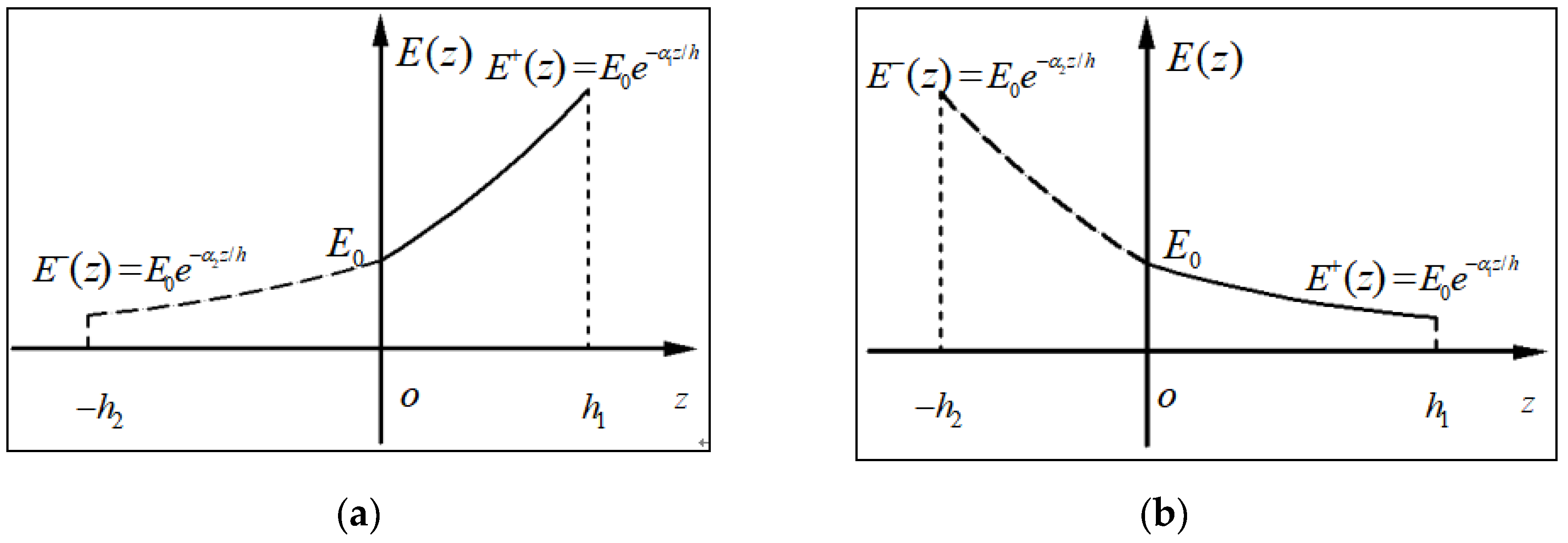
For the determination of the tensile and compressive height of the beam, a set of functionally-graded indexes should be chosen first in the light of our previous study on static analysis [28]. In this study, we consider the following two groups of gradient indexes: (a) ${\alpha }_1=-2,{\alpha }_2=-3$ and (b) ${\alpha }_1=2,{\alpha }_2=3$ to correspond to the two different cases: $E^{+}(z)>E^{-}(z)$ as well as $E^{-}(z)>E^{+}(z)$, respectively, as shown in Figure 3, in which $E_0$ is the electric modulus value on the neutral layer, in case (a), $h_1=0.6\mathrm{mm}$, $h_2=1.4\mathrm{mm}$ and in case (b), $h_1=1.4\mathrm{mm}$, $h_2=0.6\mathrm{mm}$.

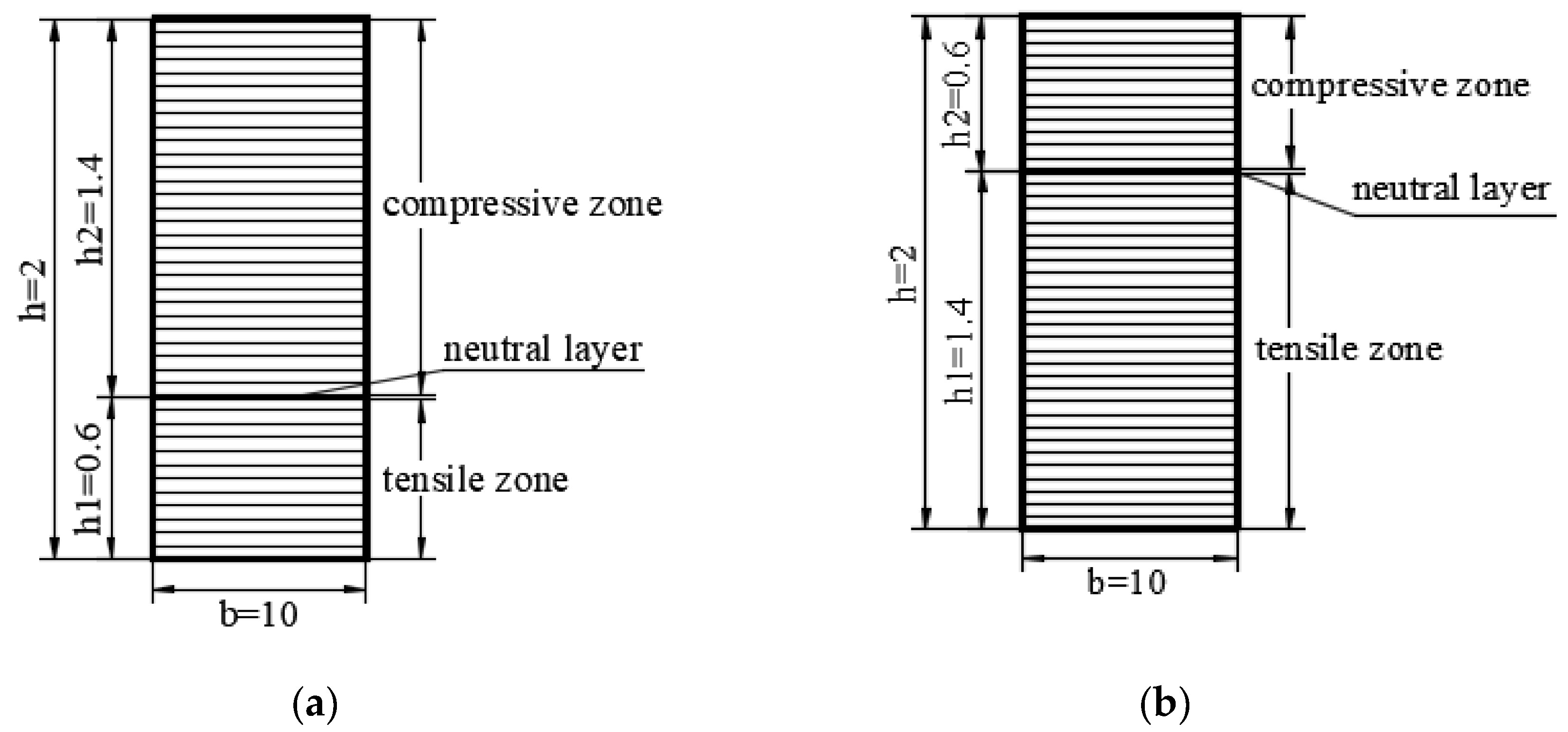
As is the case in most commercial software, there will be the limitations for implementing FGMs in ABAQUS; for example, it seems to be inconvenient to realize the change of material properties along a certain direction as a continuous function. To overcome the shortcomings, an alternative implementation was proposed in the context of the commercial finite element package ABAQUS [31]. In this study, however, the layer-wise model was still used to simulate the functionally-graded properties, since this practice is conventional and well-known. Without losing the computational accuracy, we divided the beam into a moderate number of layers along the thickness direction; the physical parameters of the material on each layer are considered to be the same, thus indirectly realizing the continuous variation of properties of materials along the thickness direction if the numbers for layering are sufficient. To this end, bound by the neutral layer, the upper and lower areas of the beam are equally divided into 40 layers along the thickness direction, each layer being 0.05 mm thick, as depicted in Figure 4. It is easy to see that in case (a), there are 28 layers in the compressive area and 12 layers in the tensile area, while in case (b), the layering is the opposite, that is, 12 layers in the compressive area and 28 layers in the tensile area. The coordinate origin is still on the neutral layer.

(iii)

Input of properties of materials

The material PbZrTiO₃-4 (generally abbreviated as PZT-4) is selected as our materials simulated.

Table 1. Elastic, piezoelectric and dielectric constants of PZT-4 materials [32].

Elastic Constant (10−12 m2·N−1)					Piezoelectric Constant (10−12 C·N−1)			Dielectric Constant (10−8 F·m−1)
$s_{11}^0$	$s_{12}^0$	$s_{13}^0$	$s_{33}^0$	$s_{44}^0$	$d_{31}^0$	$d_{33}^0$	$d_{15}^0$	${\lambda }_{11}^0$	${\lambda }_{33}^0$
12.4	−3.98	−5.52	16.1	39.1	−135	300	525	1.301	1.151

shows the material constant on the neutral layer $z=0$ which are directly input into ABAQUS. Material constants up or down the neutral layer may be computed and input into the program, by using the layering pattern of tension-compression established in Step (ii).

(iv)

Boundary conditions

The left end of the beam is fully fixed and the right end is free; this agrees with the mechanical model presented in Figure 2. Besides, the upper and lower surfaces of the beam are open circuited.

(v)

Mesh division

An 8-node linear piezoelectric brick C3D8E is used, and the mesh size is set to be $1\mathrm{mm}\times 1\mathrm{mm}$, in which the size ratio is 0.001 and also the global seed is set.

4.3. Analysis of Frequency Extraction

While solving linear dynamic problems, the mode superposition method is used in ABAQUS. Before the dynamic analysis, we need to extract the frequency of the computational example to obtain the vibration mode and natural frequency of the structure.

First of all, according to the initial model established in Section 4.2, the density of materials is defined as $7.5\times {10}^3{\mathrm{kg}/\mathrm{m}}^3$ in a property function module and also the frequency extraction analysis is defined in the analysis step. In ABAQUS, there are two kinds of method in the frequency extraction: one is the Lanczos method, which is suitable for the larger model and needs to extract the multi-order mode; the other is the subspace iterative method. In this computation, the latter is selected due to the characteristic of structural unit.

In the analysis of linear dynamic problems using the mode superposition method, a sufficient number of modes are required in the frequency extraction. The criterion follows that the total effective mass in the main direction of motion exceeds 90% of the movable mass in the model. To this end, we calculate and extract the frequency whose eigenvalue numbers are 10, 15 and 20, respectively, to select the appropriate eigenvalue. By viewing DAT file, we extract the data of frequency, participation factors and effective mass for 10, 15 and 20 eigenvalues, as shown in

Table 2. Frequency, participation factor and effective mass for 10 eigenvalues.

	Mode Number	Frequency/Hz (Cycles Time)	Participation Factor (z-component)	Effective Mass/Kg (z-component)
	1	326.490	1.565	4.562 × 10−3
	2	1767.500	6.332 × 10−11	7.519 × 10−24
	3	2029.300	−0.868	1.418 × 10−3
	4	2688.300	2.535 × 10−10	8.065 × 10−23
	5	5634.600	0.510	4.941 × 10−4
	6	7994.700	8.990 × 10−9	1.007 × 10−19
	7	9720.000	−2.243 × 10−8	1.114 × 10−18
	8	10,916.000	−0.366	2.549 × 10−4
	9	13,994.000	−4.504 × 10−6	1.983 × 10−14
	10	14,237.000	1.494 × 10−2	8.313 × 10−7
Total				6.729 × 10−3

,

Table 3. Frequency, participation factor and effective mass for 15 eigenvalues.

	Mode Number	Frequency/Hz (Cycles Time)	Participation Factor (z-component)	Effective Mass/Kg (z-component)
	1	326.490	1.565	4.562 × 10−3
	2	1767.500	6.332 × 10−11	7.519 × 10−24
	3	2029.300	−0.868	1.418 × 10−3
	4	2688.300	2.527 × 10−10	8.016 × 10−23
	5	5634.600	0.510	4.941 × 10−4
	……	……	……	……
	12	20,587.000	−7.667 × 10−7	5.125 × 10−16
	13	22,745.000	−1.099 × 10−6	3.228 × 10−15
	14	26,094.000	−0.244	1.042 × 10−4
	15	28,006.000	−2.242 × 10−5	3.993 × 10−13
Total				6.989 × 10−3

and

Table 4. Frequency, participation factor and effective mass for 20 eigenvalues.

	Mode Number	Frequency/Hz (Cycles Time)	Participation Factor (z-component)	Effective Mass/Kg (z-component)
	1	326.490	1.565	4.562 × 10−3
	2	1767.500	6.331 × 10−11	7.517 × 10−24
	3	2029.300	−0.868	1.418 × 10−3
	4	2688.300	2.527 × 10−10	8.016 × 10−23
	5	5634.600	0.510	4.941 × 10−4
	……	……	……	……
	17	36,310.000	4.508 × 10−7	1.586 × 10−16
	18	37,469.000	4.075 × 10−7	5.328 × 10−16
	19	42,285.000	1.940 × 10−2	1.246 × 10−6
	20	45,307.000	0.236	3.677 × 10−5
Total				7.101 × 10−3

. Here, below, are listed the data from the case ${\alpha }_1=-2,{\alpha }_2=-3$, which is very significant.

The main motion direction of the beam is along the z-axis direction, the participation factors in Table 2, Table 3 and Table 4 reflect that the first-order mode acts mainly in the z-direction. The total mass of this model is $7.500\times {10}^{-3}\mathrm{kg}$. Since the constrained nodes account for a small proportion of all nodes, it may be approximated that the movable mass in the model is equal to the total of the model.

Table 5. Ratios of z-direction mass to total mass under different eigenvalue numbers.

Eigenvalue Numbers	Effective z-Direction Movable Mass to Total Motion Mass
10	$6.729\times {10}^{-3}/(7.500\times {10}^{-3})=89.72\%$
15	$6.989\times {10}^{-3}/(7.500\times {10}^{-3})=93.19\%$
20	$7.101\times {10}^{-3}/(7.500\times {10}^{-3})=94.68\%$

shows that, when eigenvalue numbers are 10, 15 and 20, respectively, the ratio of effective mass in z-direction to total motion mass. It is easy to see that when the eigenvalue numbers are 15 and 20, the ratios are uniformly greater than 90%, which both satisfy the basic requirement for sufficient number of modes. However, considering the hardware factors and amount of calculation, the 15th order mode is adopted here. Besides, for another case ${\alpha }_1=2,{\alpha }_2=3$, we still select the 15th order mode, the ratio reads $6.993\times {10}^{-3}/(7.500\times {10}^{-3})=93.24\%$ in this case.

4.4. Simulation for Free Damping Vibration

As shown in Table 3, we have finished the frequency extraction of 15 eigenvalues for the case ${\alpha }_1=-2,{\alpha }_2=-3$, in which the maximum frequency reads 28,006 Hz; thus, the corresponding period is $1/28006\mathrm{s}=0.00003571\mathrm{s}$. Since the time increment in the analysis step of transient modal should be less than this period value, the time increment is determined as $3\times {10}^{-5}\mathrm{s}$. The details are shown below.

(i)

Establishment of dynamic analysis step of transient modal

Although the material properties considered in this study are bimodular, functionally-graded and piezoelectric—that is, it is not linear—the nonlinear behavior of the material itself has little impact on the dynamic response of the structure. Besides, the motion attributes to the small deflection bending vibration thus there is no geometrical nonlinearity here. Furthermore, the damping of the structural system is relatively small, and the frequency involved in the analysis is low. Therefore, the system may be regarded as linear, which is suitable for linear transient dynamic analysis.

Frequency extraction analysis step is followed by this step. To observe the attenuation process of the vibration, the analytical step time is set to be 0.5 s and the time increment is determined as $3\times {10}^{-5}\mathrm{s}$, as indicated above.

(ii)

Setting of the damping

Direct modal damping is used here and the value of the damping ratio is 0.03. The starting mode order is 1 and the terminating mode order is 15.

(iii)

Setting of the output of historical variable

In the output of historical variable, the displacement component is selected.

(iv)

Definition of load

In order to make the model produce the initial displacement of 2 mm, a short-term load is applied on the model, in which the time of duration of the load is determined by the variation of load amplitudes with time and the amplitude is given in tabulate. In the time period 0–0.005 s, the amplitude is 1; and in the later time period, the amplitude is set as 0. The smoothness parameter is set as 0.25. Lastly, along the negative direction of z-axis, the load is applied and the magnitude of the load is 25 N.

(v)

Submission of analysis and post-processing

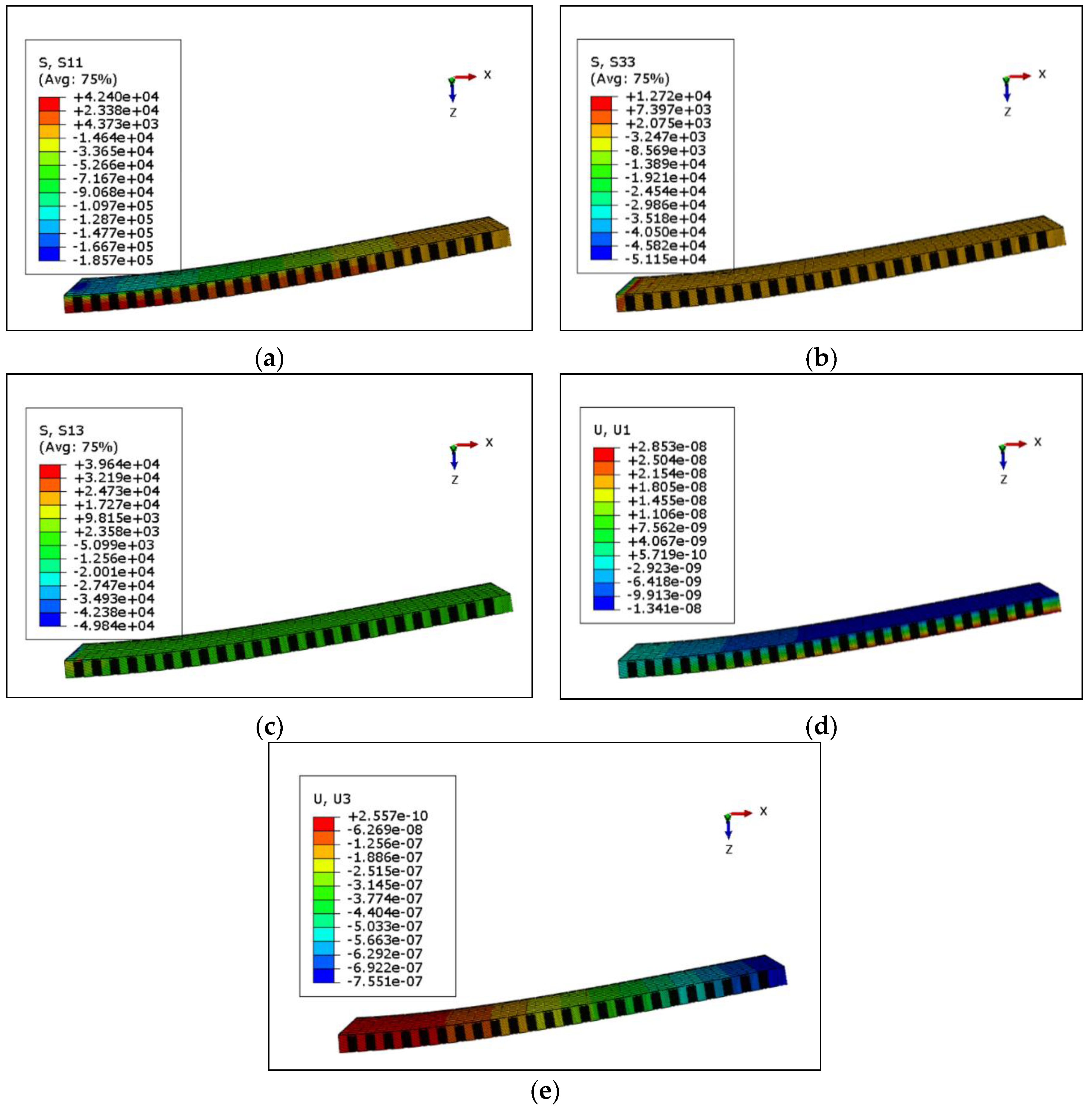
After a job is established, we may submit the job and calculate and output the results. Figure 5 and Figure 6 show cloud diagrams of stress and displacement of 15th order mode at the end of the transient modal analysis, in which Figure 5 is for the case ${\alpha }_1=-2,{\alpha }_2=-3$ and Figure 6 is for the case ${\alpha }_1=2,{\alpha }_2=3$.

Note that although the numerical implementation in ABAQUS is three-dimensional in the form, we still put out the final results in the form of two-dimensional case, including three stresses, ${\sigma }_x$, ${\sigma }_z$ and ${\tau }_{xz}$, as well as two displacements, $u$ and $w$, which are typical in two-dimensional plane problem. In fact, the studied problem is a two-dimensional plane problem, even in some cases (for example, a slim beam), the problem may be further simplified as a one-dimensional problem, like our analytical solution based on Euler–Bernoulli beam theory.

5. Comparisons and Discussion

5.1. Comparison of Theoretical and Numerical Results

For the purpose of the full comparison between the theoretical results and numerical ones, both under the two cases of different modulus—that is, the tensile elastic modulus is greater than the compressive one $E^{+}(z)>E^{-}(z)$, or reversely, $E^{+}(z)<E^{-}(z)$—we should select an object of study from the beam, for example, the upper surface of the free end, as our study object. In order to investigate the displacement variation with time under two cases of different modulus, we take the following two cases of functionally-grade index: (a) ${\alpha }_1=-2,{\alpha }_2=-3$, which corresponds to $E^{+}(z)>E^{-}(z)$, and the case (b) ${\alpha }_1=2,{\alpha }_2=3$, which corresponds to $E^{+}(z)<E^{-}(z)$. The numerical results are taken from the 15th order mode. For the theoretical results, we should compute the equivalent modulus of elasticity first. For this purpose, substituting Equation (1) into Equation (8), we have

$$E^{*}=\frac{{\lambda }_{33}^{+/-}}{s_{11}^{+/-}{\lambda }_{33}^{+/-}-{(d_{31}^{+/-})}^2}=\frac{{\lambda }_{33}^0}{s_{11}^0{\lambda }_{33}^0-{(d_{31}^0)}^2}{e}^{-{\alpha }_{i}z/h}$$

(26)

Substituting the values of $s_{11}^0$, $d_{31}^0$ and ${\lambda }_{33}^0$ from Table 1 into the above equation and also noting that the upper surface is in compression; thus, ${\alpha }_i={\alpha }_2$, the values of the equivalent modulus of elasticity, may be determined and is listed in

Table 6. Equivalent modulus and frequency from theoretical and numerical results.

Cases	Equivalent Modulus ${\mathit{E}}^{*}$ (GPa)	Vibration Frequency $\mathit{\omega }$ (Hz)
		Theoretical Value	Numerical Value
$E^{+}(z)>E^{-}(z)$	11	17,506	28,006
$E^{+}(z)<E^{-}(z)$	227	28,019	34,599

. Note that for the first case, $E^{+}(z)>E^{-}(z)$, we take ${\alpha }_i={\alpha }_2=-3$ and $z=-0.0014\mathrm{m}$, and for the second case, $E^{+}(z)<E^{-}(z)$, we have ${\alpha }_i={\alpha }_2=3$ and $z=-0.0006\mathrm{m}$, in which the values of z may refer to the cases (a) and (b) in Figure 4. Besides, the theoretical value of vibration frequency may be obtained via the expression ${\omega }^2=a^4{E}^{*}{I}^y/\overline{m}$ and the numerical result of frequency is also from the 15th order modes, which are also listed in Table 6.

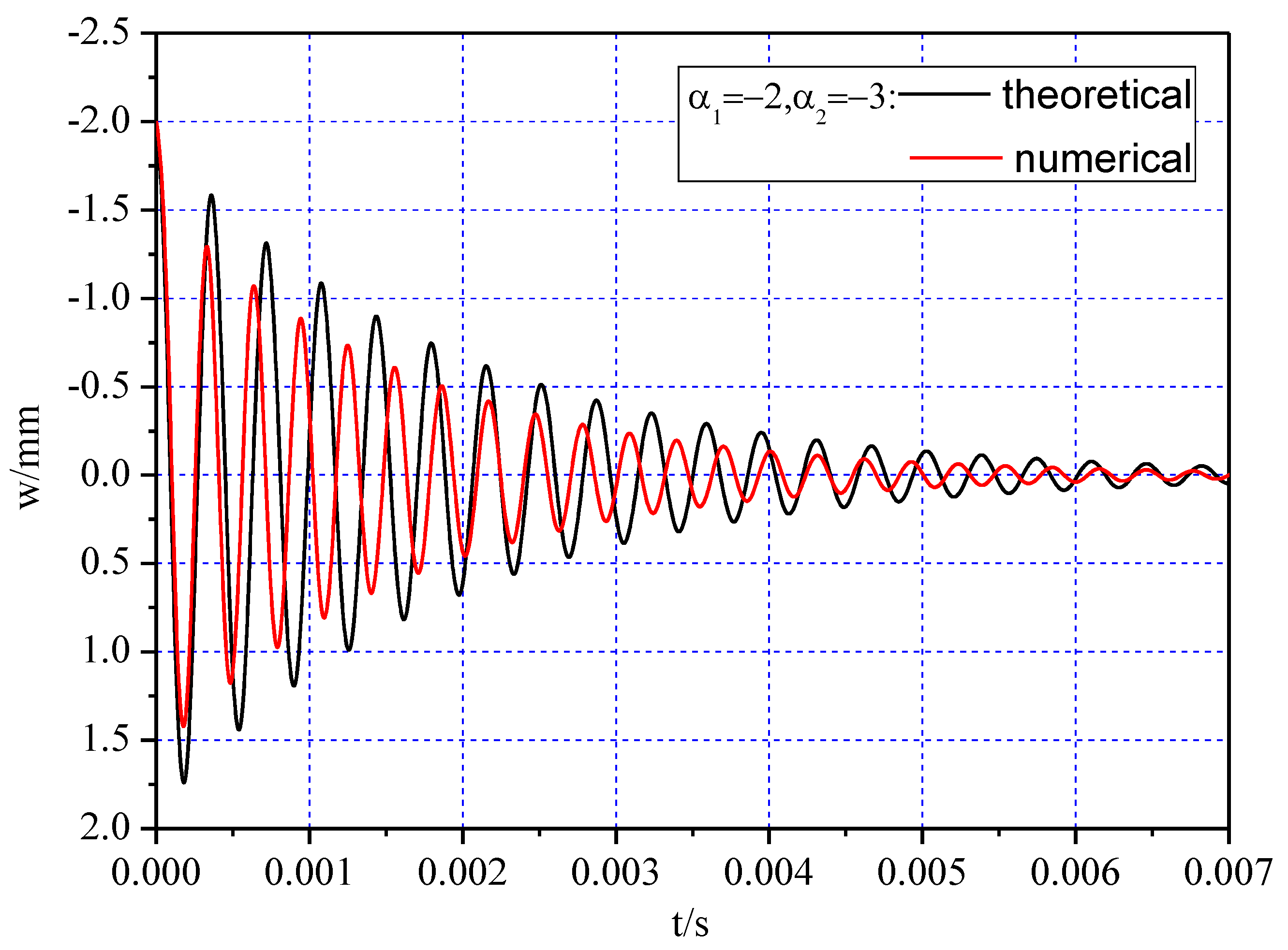
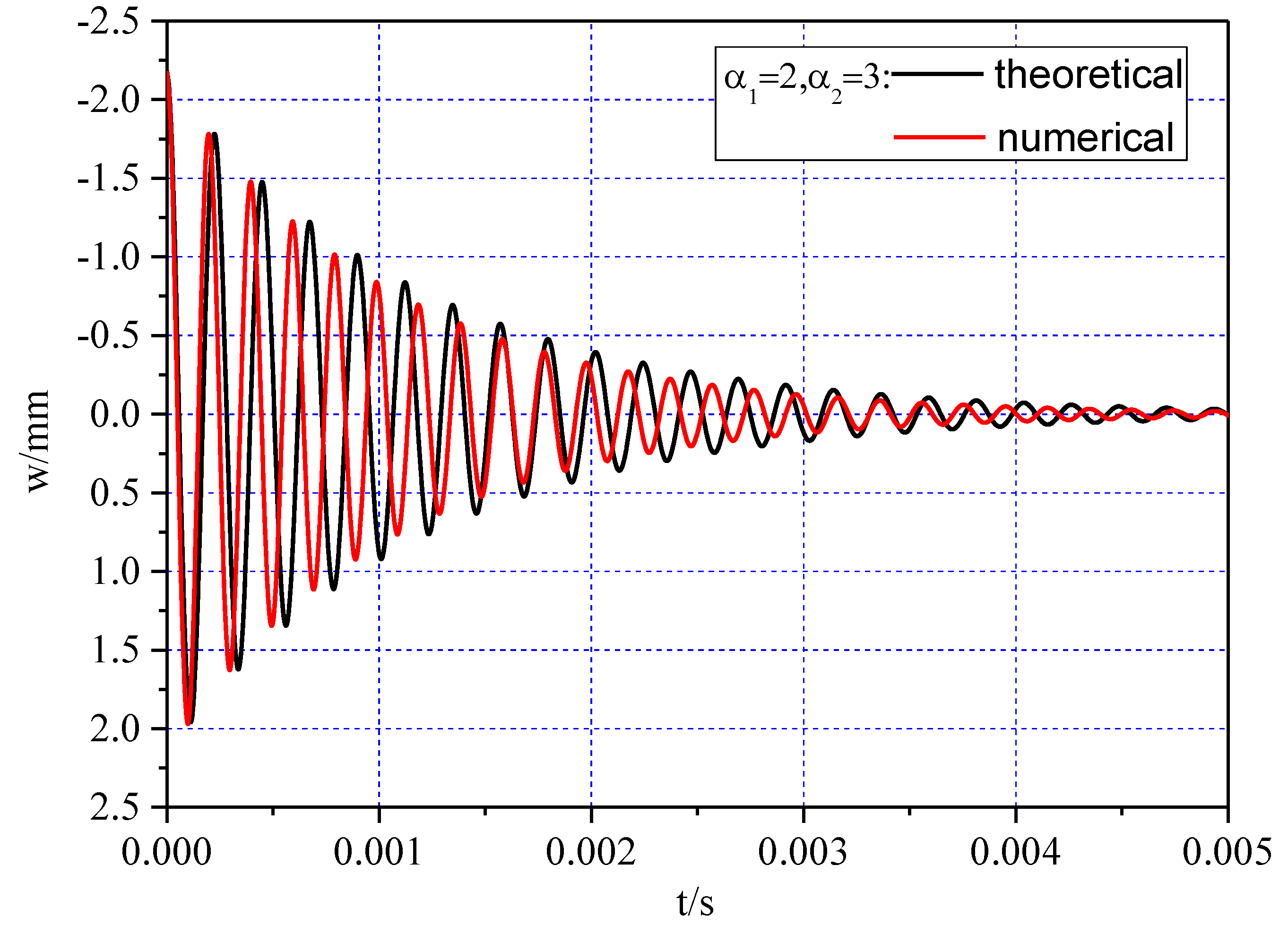
Figure 7 and Figure 8 show the two time-displacement curves from theoretical and numerical results, in which Figure 7 is for $E^{+}(z)>E^{-}(z)$ and Figure 8 is for $E^{+}(z)<E^{-}(z)$. It is easy to see that despite some differences, the theoretical curve basically agrees with the curve from numerical simulation, this validates the theoretical solution to some extent.

From Figure 7 and Figure 8, we may also see that under two cases $E^{+}(z)>E^{-}(z)$ and $E^{+}(z)<E^{-}(z)$, the attenuation speed of the vibration from the numerical result is faster than that from theoretical solution, this is because the natural frequency from numerical simulation is greater than the one from theoretical solution, which may be easily seen from Table 6, in which for $E^{+}(z)>E^{-}(z)$, the value from numerical simulation is 28,006 Hz while the counterpart from theoretical solution is 17,506 Hz; for $E^{+}(z)<E^{-}(z)$, the two values from numerical simulation and theoretical solution are 34,599 Hz and 28,019 Hz, respectively. In addition, for $E^{+}(z)<E^{-}(z)$, the attenuation speed is obviously faster than that in the case $E^{+}(z)>E^{-}(z)$; this also may be easily seen from Table 6, in which the natural frequency from $E^{+}(z)<E^{-}(z)$ is greater than the one from $E^{+}(z)>E^{-}(z)$, for example, for theoretical solutions 28,019 Hz is greater than 17,506 Hz, while the numerical simulation 34,599 Hz is also greater than 28,006 Hz. It may be concluded that the relative magnitudes of the tensile and compressive moduli have influence on the attenuation speed of the vibration.

It should be noted here that there are some differences between the theoretical solution and the numerical simulation, mainly due to the different mechanical models on which the two methods are established. In the theoretical analysis, the introduction of the equivalent modulus of elasticity may greatly simplify the derivation process; on the other hand, this equivalent practice inevitably cause some errors, in other words, the so-called equivalence is actually a compromise. Based on this consideration, the numerical simulation seems to be more accurate than the theoretical analysis; that is to say, the theoretical analysis and numerical simulation have their own advantages and complement each other.

5.2. Comparison of Theoretical and Experimental Results

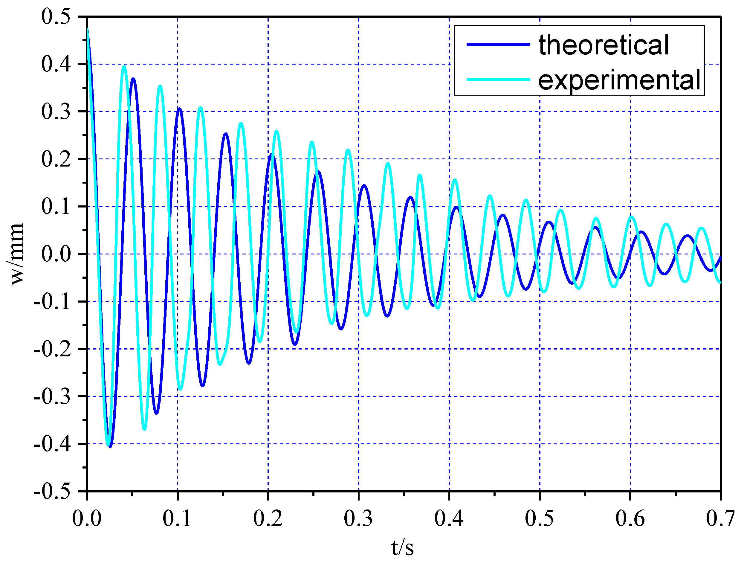
At present, the relevant vibration experiment for the functionally-graded piezoelectric cantilever beam has not been found, not to mention the consideration for bimodular effect of the materials. The comparison should therefore be based on the experimental data available. Aiming at purely piezoelectric materials (which means there is no bimodular effect and also no functionally-graded characteristic), Yang et al. [33] performed an experiment of free damping vibration of a cantilever beam. In this section, the theoretical solution derived in this study with the experimental results from [33] will be compared.

Before comparison, it is necessary for us to reduce our theoretical solution to a purely piezoelectric case, to agree with the material model adopted in [33]. For this purpose, we need to presume ${\alpha }_1={\alpha }_2=0$ in Equation (8); thus, the equivalent modulus of elasticity $E^{*}$ may be simplified as

$$E^{\prime }=\frac{{\lambda }_{33}^{}}{s_{11}^{}{\lambda }_{33}^{}-{(d_{31}^{})}^2}$$

(27)

in which $E^{\prime }$ stands for the equivalent modulus of elasticity without bimodular and functionally-graded characteristic. Accordingly, Equation (18) may be changed as

$${\omega }_D^{\prime }={\omega }^{\prime }\sqrt{1-{\xi }^2}$$

(28)

in which ${\omega }_D^{\prime }$ is the natural damped frequency in the same case of materials.

In the comparison we should take the same parameters in accordance with the experimental model in [33], including the shape dimension of the beam, $h=0.0001$ m, $b=0.02$ m, $l=0.05$ m, the damping ration $\xi =0.03$ and the uniformly-distributed mass $\overline{m}=0.015$ Kg/m, as well as the material parameters of PZT-5 (shown in

Table 7. Materials parameters of PZT-5 [33].

Elastic Constant (10−12 m2·N−1)					Piezoelectric Constant (10−12 C·N−1)			Dielectric Constant (10−8 F·m−1)
$s_{11}$	$s_{12}$	$s_{13}$	$s_{33}$	$s_{44}$	$d_{31}$	$d_{33}$	$d_{15}$	${\lambda }_{11}$	${\lambda }_{33}$
16.4	−5.74	−7.22	18.8	47.5	−172	374	584	1.505	1.531

). Besides, three different initial displacements in [33] are also adopted in our theoretical results; thus,

Table 8. Frequencies of experimental and theoretical results.

Initial Displacements (mm)	Vibration Frequency (Hz)
	Experimental Results Reference [33]	Theoretical Results (This Paper)	Relative Errors (%)
0.475	123.25	123.220	0.02
0.750	123.25	123.220	0.02
1.342	123.25	123.220	0.02

lists the vibration frequencies from experimental measurement and theoretical solution. It is easily seen that the differences between experimental results and theoretical results are small, which indicates the theoretical vibration frequency is reliable.

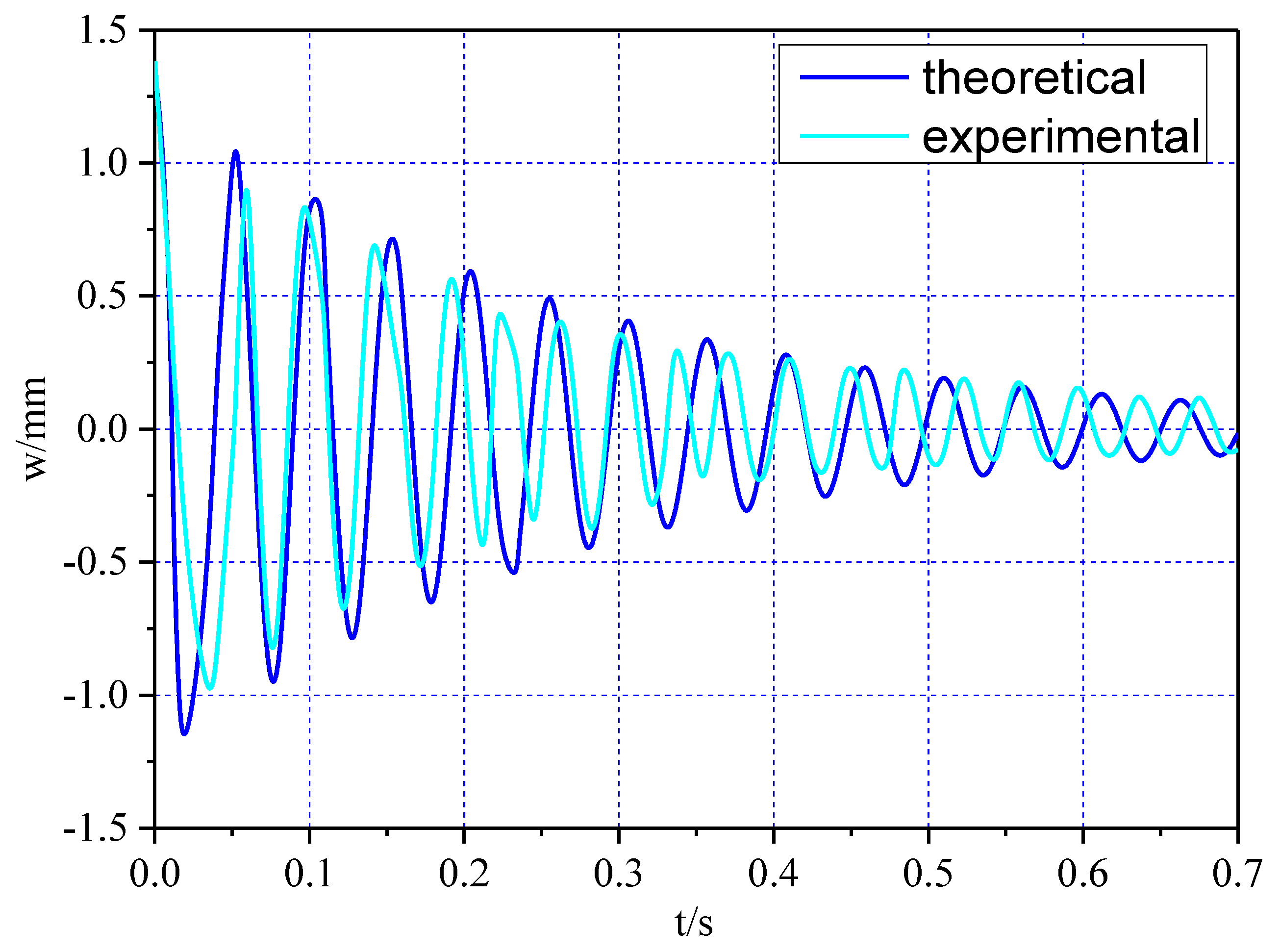
Figure 9, Figure 10 and Figure 11 show time-displacement curves from theoretical and experimental results under the three different initial displacements. It is readily found that the theoretical results agree with the experimental ones, although there are some differences between them, which may be caused by some uncontrollable factors in the experimental operation.

6. Conclusions

In this study, we investigate the free damping vibration problem of a bimodular FGPM cantilever beam by using analytical and numerical methods. By comparisons, the theoretical results basically agree with the numerical results, although there are some differences, mainly due to the different mechanical models. In addition, the theoretical solutions after regression agree well with the experimental results of the pure piezoelectric cantilever, which also proves, indirectly, the effectiveness of theoretical work. The following three conclusions can be drawn:

(i)

Under two cases, $E^{+}(z)>E^{-}(z)$ and $E^{+}(z)<E^{-}(z)$, the attenuation speed of the vibration from numerical simulation is faster than that from theoretical solution; besides, the attenuation speed in the case $E^{+}(z)<E^{-}(z)$ is obviously faster than that in the case $E^{+}(z)>E^{-}(z)$.

(ii)

The bimodular functionally-graded properties may change, to some extent, the dynamic response of the piezoelectric cantilever beam; however, the influence could be relatively small and unobvious.

(iii)

In the frame of simple models, with analytical considerations, this work may be helpful for the analysis and design of flexible and lightweight cantilever-type elements composed of piezoelectric materials, especially when the bimodular functionally-graded properties of materials cannot be completely ignored.

Although the results in this study are obtained on the piezoelectric ceramics (PZT), this work will also be helpful for predicting the mechanical behaviors of a vibrational cantilever made of piezoelectric polymer films (PVDF); however, there may be a huge difference in their behavior and property about vibrational cantilever. Among the two main types of piezoelectric materials, due to the fact that the elastic modulus of PZT is far greater than that of PVDF; thus, the vibration frequency of PZT is far greater than that of PVDF. This should be give more attention in analyzing the vibration characteristic of cantilevers made of the two different piezoelectric materials.

References

- Yeo, H.G.; Ma, X.; Rahn, C.; Trolier-McKinstry, S. Efficient piezoelectric energy harvesters utilizing (001) textured bimorph PZT films on flexible metal foils. Adv. Funct. Mater. 2016, 26, 5940–5946. [Google Scholar] [CrossRef]
- Won, S.S.; Seo, H.; Kawahara, M.; Glinsek, S.; Lee, J.; Kim, Y.; Jeong, C.K.; Kingon, A.I.; Kim, S.H. Flexible vibrational energy harvesting devices using strain-engineered perovskite piezoelectric thin films. Nano Energy 2019, 55, 182–192. [Google Scholar] [CrossRef]
- Huang, D.J.; Ding, H.J.; Chen, W.Q. Piezoelasticity solutions for functionally-graded piezoelectric beams. Smart Mater. Struct. 2007, 16, 687–695. [Google Scholar] [CrossRef]
- Bodaghi, M.; Damanpack, A.R.; Aghdam, M.M.; Shakeri, M. Geometrically non-linear transient thermo-elastic response of FG beams integrated with a pair of FG piezoelectric sensors. Compos. Struct. 2014, 107, 48–59. [Google Scholar] [CrossRef]
- Kulikov, G.M.; Plotnikova, S.V. An analytical approach to three-dimensional coupled thermoelectroelastic analysis of functionally-graded piezoelectric plates. J. Intell. Mater. Syst. Struct. 2017, 28, 435–450. [Google Scholar] [CrossRef]
- Alibeigloo, A. Thermo elasticity solution of functionally-graded, solid, circular, and annular plates integrated with piezoelectric layers using the differential quadrature method. Mech. Adv. Mater. Struct. 2018, 25, 766–784. [Google Scholar] [CrossRef]
- Heydarpour, Y.; Malekzadeh, P.; Dimitri, R.; Tornabene, F. Thermoelastic analysis of functionally graded cylindrical panels with piezoelectric layers. Appl. Sci. 2020, 10, 1397. [Google Scholar] [CrossRef] [Green Version]
- Arefi, M.; Bidgoli, E.M.R.; Dimitri, R.; Bacciocchi, M.; Tornabene, F. Application of sinusoidal shear deformation theory and physical neutral surface to analysis of functionally graded piezoelectric plate. Compos. Part B Eng. 2018, 151, 35–50. [Google Scholar] [CrossRef]
- Mahinzare, M.; Ranjbarpur, H.; Ghadiri, M. Free vibration analysis of a rotary smart two directional functionally-graded piezoelectric material in axial symmetry circular nanoplate. Mech. Syst. Signal Process. 2018, 100, 188–207. [Google Scholar] [CrossRef]
- Yao, R.X.; Shi, Z.F. Steady-State forced vibration of functionally-graded piezoelectric beams. J. Intell. Mater. Syst. Struct. 2011, 22, 769–779. [Google Scholar] [CrossRef]
- Shakeri, M.; Mirzaeifar, R. Static and dynamic analysis of thick functionally-graded plates with piezoelectric layers using layerwise finite element model. Mech. Adv. Mater. Struct. 2009, 16, 561–575. [Google Scholar] [CrossRef]
- Ebrahimi, F. Analytical investigation on vibrations and dynamic response of functionally-graded plate integrated with piezoelectric layers in thermal environment. Mech. Adv. Mater. Struct. 2013, 20, 854–870. [Google Scholar] [CrossRef]
- Chen, M.F.; Chen, H.L.; Ma, X.L.; Jin, G.Y.; Ye, T.G.; Zhang, Y.T.; Liu, Z.G. The isogeometric free vibration and transient response of functionally-graded piezoelectric curved beam with elastic restraints. Results Phys. 2018, 11, 712–725. [Google Scholar] [CrossRef]
- Li, S.R.; Su, H.D.; Cheng, C.J. Free vibration of functionally-graded material beams with surface-bonded piezoelectric layers in thermal environment. Appl. Math. Mech. 2009, 30, 969–982. [Google Scholar] [CrossRef]
- Huang, X.L.; Shen, H.S. Vibration and dynamic response of functionally-graded plates with piezoelectric actuators in thermal environments. J. Sound Vib. 2006, 289, 25–53. [Google Scholar] [CrossRef]
- Fu, Y.; Wang, J.; Mao, Y. Nonlinear analysis of buckling, free vibration and dynamic stability for the piezoelectric functionally-graded beams in thermal environment. Appl. Math. Modell. 2012, 36, 4324–4340. [Google Scholar] [CrossRef]
- Li, Y.; Shi, Z. Free vibration of a functionally-graded piezoelectric beam via state-space based differential quadrature. Compos. Struct. 2009, 87, 257–264. [Google Scholar] [CrossRef]
- Barak, M.M.; Currey, J.D.; Weiner, S.; Shahar, R. Are tensile and compressive Young’s moduli of compact bone different. J. Mech. Behav. Biomed. Mater. 2009, 2, 51–60. [Google Scholar] [CrossRef]
- Destrade, M.; Gilchrist, M.D.; Motherway, J.A.; Murphy, J.G. Bimodular rubber buckles early in bending. Mech. Mater. 2010, 42, 469–476. [Google Scholar] [CrossRef] [Green Version]
- Jones, R.M. Stress–strain relations for materials with different moduli in tension and compression. AIAA J. 1977, 15, 16–23. [Google Scholar] [CrossRef]
- Ambartsumyan, S.A. Elasticity Theory of Different Moduli; Wu, R.F.; Zhang, Y.Z., Translators; China Railway Publishing House: Beijing, China, 1986. [Google Scholar]
- Zhang, Y.Z.; Wang, Z.F. Finite element method of elasticity problem with different tension and compression moduli. Comput. Struct. Mech. Appl. 1989, 6, 236–245. [Google Scholar]
- Ye, Z.M.; Chen, T.; Yao, W.J. Progresses in elasticity theory with different moduli in tension and compression and related FEM. Mech. Eng. 2004, 26, 9–14. [Google Scholar]
- Sun, J.Y.; Zhu, H.Q.; Qin, S.H.; Yang, D.L.; He, X.T. A review on the research of mechanical problems with different moduli in tension and compression. J. Mech. Sci. Technol. 2010, 24, 1845–1854. [Google Scholar] [CrossRef]
- Du, Z.L.; Zhang, Y.P.; Zhang, W.S.; Guo, X. A new computational framework for materials with different mechanical responses in tension and compression and its applications. Int. J. Solids Struct. 2016, 100, 54–73. [Google Scholar] [CrossRef]
- He, X.T.; Li, Y.H.; Liu, G.H.; Yang, Z.X.; Sun, J.Y. Non-linear bending of functionally graded thin plates with different moduli in tension and compression and its general perturbation solution. Appl. Sci. 2018, 8, 731. [Google Scholar]
- He, X.T.; Wang, Y.Z.; Shi, S.J.; Sun, J.Y. An electroelastic solution for functionally-graded piezoelectric material beams with different moduli in tension and compression. J. Intell. Mater. Syst. Struct. 2018, 29, 1649–1669. [Google Scholar] [CrossRef]
- He, X.T.; Yang, Z.X.; Jing, H.X.; Sun, J.Y. One-dimensional theoretical solution and two-dimensional numerical simulation for functionally-graded piezoelectric cantilever beams with different properties in tension and compression. Polymers 2019, 11, 1728. [Google Scholar]
- Yu, T.; Zhong, Z. Bending analysis of a functionally-graded piezoelectric cantilever beam. Sci. China Ser. G Phys. Mech. Astron. 2007, 50, 97–108. [Google Scholar] [CrossRef]
- Clough, R.W.; Penzien, J. Dynamics of Structures, 2nd ed.; Wang, G.Y., Translator; Higher Education Press: Beijing, China, 2006. [Google Scholar]
- Martínez-Pañeda, E. On the finite element implementation of functionally graded materials. Materials 2019, 12, 287. [Google Scholar] [CrossRef] [Green Version]
- Ruan, X.P.; Danforth, S.C.; Safari, A.; Chou, T.W. Saint-Venant end effects in piezoceramic materials. Int. J. Solids Struct. 2000, 37, 2625–2637. [Google Scholar] [CrossRef]
- Yang, Z.X.; He, X.T.; Peng, D.D.; Sun, J.Y. Free damping vibration of piezoelectric cantilever beams: A biparametric perturbation solution and its experimental verification. Appl. Sci. 2020, 10, 215. [Google Scholar] [CrossRef] [Green Version]
Figure 1.
Constitutive model for bimodular materials: (a) nonlinear model under actual state; (b) bilinear model when ; (c) bilinear model when .
Figure 2.
Scheme of the functionally-graded piezoelectric materials (FGPM) bimodular cantilever beam.
Figure 3.
: (a) , ; (b) , .
Figure 4.
Sketch of layering on cross section of the beam (unit: mm): (a) , ; (b) , .
Figure 5.
Cloud diagram of stress and displacement for the case , : (a); (b); (c); (d); (e).
Figure 6.
Figure 7.
Comparison of two time-displacement curves for
Figure 8.
Figure 9.
Comparison of two time-displacement curves under initial displacement 0.475 mm.
Figure 10.
Comparison of two time-displacement curves under initial displacement 0.750 mm.
Figure 11.
Comparison of two time-displacement curves under initial displacement 1.342 mm.