Decentralized Adaptive Tracking of Interconnected Nonlinear Systems by Corrupted Output Feedback


School of Electrical and Electronics Engineering, Chung-Ang University, 84 Heukseok-Ro, Dongjak-Gu, Seoul 06974, Korea
*
Author to whom correspondence should be addressed.
Mathematics 2020, 8(8), 1340; https://doi.org/10.3390/math8081340
Submission received: 8 July 2020
/
Revised: 28 July 2020
/
Accepted: 10 August 2020
/
Published: 11 August 2020
Abstract
:A decentralized adaptive resilient output-feedback stabilization strategy is presented for a class of uncertain interconnected nonlinear systems with unknown time-varying measurement sensitivities. In the concerned problem, the main difficulty is to achieve the decentralization of interconnected output nonlinearities unmatched to the control input by using only local output information corrupted by measurement sensitivity, namely the exact output information cannot be used to design the decentralized output-feedback control scheme. Thus, a decentralized output-feedback stabilizer design using only the corrupted output of each subsystem is developed where the adaptive control technique is employed to compensate for the effects of unknown measurement sensitivities. The stability of the resulting decentralized control scheme is analyzed based on the Lyapunov stability theorem.
1. Introduction
For the implementation of control systems, sensors play a crucial role in measuring the state variables of physical systems, and thus, the measurement precision of the sensor affects the control performance [1]. However, due manufacturing reasons or the practical limitations of sensors, the measured state variables can be inaccurate in the practical environment [2,3]. Therefore, a main issue is to design stable controllers regardless of the inaccurate measurement of sensors. In [4,5,6,7,8,9,10,11,12], there were attempts to control single linear or nonlinear systems with uncertain measurement sensitivity. Output-feedback control approaches were proposed via the feedback domination approach [6,7,8,9,10], and a sampled data output-feedback stabilizer was developed in [11]. In [12], the output-feedback controller using the dual-domination approach was designed for nonlinear systems with unknown time-varying measurement sensitivity. However, these control approaches require the knowledge about the bounds of the partial derivatives of unknown output functions [6,7,8,9,10,11] and the bounds of unknown time-varying measurement sensitivity [12].
The decentralized control problem of interconnected nonlinear systems has been regarded as an interesting issue because of the benefits of decentralized controllers over standard centralized controllers such as the simplicity and computational efficiency by using the information on the subsystem itself (see [13,14,15,16,17,18] and the references therein). Among them, the adaptive recursive control techniques such as backstepping [19] and dynamic surface control [20] have been employed to handle unknown interaction nonlinearities unmatched to local control inputs [21,22,23,24,25,26]. In [27], a decentralized output-feedback domination design approach was investigated for uncertain nonlinear large-scale systems. In [28,29], decentralized adaptive control strategies were established for a class of interconnected nonlinear systems with completely unknown actuator failures. A decentralized adaptive controller was developed for interconnected nonlinear systems with stochastic disturbance [30]. An adaptive decentralized control method using barrier Lyapunov functions was proposed for uncertain large-scale nonlinear systems subject to full state constraints [31]. However, the existing results [21,22,23,24,25,26,27,28,29,30,31] did not consider the measurement sensitivity problem. Namely, the decentralization of the control structure is based on the accurate state-feedback information. The main design difficulty in considering measurement sensitivity comes from the difference between the interconnected state information of systems and the local state information used for the feedback control. Different from the state information in the interaction nonlinearities, the state information for the local control design is corrupted by measurement sensitivity. Thus, contrary to [21,22,23,24,25,26,27,28,29,30,31], the local controller using corrupted state variables should be designed for each subsystem. Because of this difficulty, there are few results to deal with the imprecise sensor measurement problem in the decentralized control field. In [32], a decentralized output-feedback small-gain controller using the cyclic-small-gain theorem was proposed to deal with the corruption of the output information owing to sensor noise. However, the previous control scheme [32] necessitates the known bound of the sensor noise.
The aim of this paper is to present a decentralized resilient output-feedback control strategy of uncertain interconnected nonlinear systems with unknown time-varying measurement sensitivities. The bounds for the measurement sensitivities are assumed to be unknown. Unmeasurable local state variables are estimated by high-gain observers using local output signals corrupted by unknown measurement sensitivities. Then, a local adaptive dynamic surface output-feedback controller for each subsystem is recursively designed using the corrupted output information where the adaptation structure is employed to compensate for unknown measurement sensitivity. In the proposed control scheme, the decentralization of interconnections among uncorrupted output signals is achieved by designing the local controller using the corrupted output information. Based on the Lyapunov stability theorem, it is ensured that all of the closed-loop signals are uniformly ultimately bounded and the local stabilization errors converge to an adjustable neighborhood of the origin in the presence of the measurement sensitivities.
The main contributions of this work are two-fold:
- (i)
- (ii)
- Compared with the existing result [32], the proposed decentralized resilient control methodology ensures the robustness on unknown time-varying measurement sensitivities, without using any bounding information of the measurement sensitivities. The adaptive control strategy is proposed to compensate for unknown bounding effects of measurement sensitivities.
The rest of the paper is organized as follows. A decentralized adaptive resilient output-feedback stabilization problem of uncertain interconnected nonlinear systems with unknown measurement sensitivities is formulated in Section 2. Local adaptive resilient output-feedback control designs and their stability analysis strategy are discussed in Section 3. Section 4 presents the simulation results. In Section 5, some conclusions are given.
2. Problem Statement
Consider interconnected nonlinear systems consisting of subsystems with unknown measurement sensitivities. The ith subsystem is represented by:
where , , , , and are the system state vector, the control input, and the system output of the ith subsystem, respectively, denotes interconnected state variables among subsystems, are nonlinear functions of the ith subsystem, and denotes an unknown parameter denoting the time-varying measurement sensitivity of the ith subsystem. When , the system (1) describes ideal interconnected nonlinear systems without measurement sensitivities that are considered in [21,22,23,24,25,26,27,28,29,30,31].
Assumption A1
([6]). The system outputs corrupted by measurement sensitivities are only measurable for feedback.
Assumption A2
Remark 1.
Assumption A3.
and of each subsystem are bounded as and where , , and are unknown positive constants and the sign of is known. Without loss of generality, we assume that .
Problem 1.
The problem of this paper is to construct local adaptive control laws using only the corrupted output for stabilizing the interconnected nonlinear system (1) with the unknown time-varying measurement sensitivity .
Remark 2.
(i) In [32], a decentralized output feedback control problem was investigated for interconnected nonlinear systems with known bounds of imprecise sensor measurement. On the contrary, the proposed adaptive output feedback control strategy deals with the completely unknown bound problem of unknown measurement sensitivities. That is, the bounds , , and for the unknown measurement sensitivities are unknown.
(ii) Assumption 2 implies that the nonlinear functions are bounded as the linear combination of state variables. According to the amplitude of uncertain nonlinear functions, the constant can be adjusted to satisfy Assumption 2. Thus, the proposed control approach can achieve good control performance under Assumption 2.
(iii) In view of the controllability, Assumption 3 is reasonable for the decentralized output feedback control problem because the measurement sensitivity cannot be zero (i.e., ) and the measurement sensitivity and its derivative should be finite (i.e., and ). In addition, under Assumption 3, the high frequency of the measurement sensitivity can be allowed.
3. Decentralized Adaptive Control Via Corrupted Output Measurement
3.1. Local High-Gain Observer Design
A local high-gain observer using the output is presented to estimate the state variables as follows:
where , , denotes an observer gain and are Hurwitz polynomial coefficients of the ith observer.
Let us define the observer errors as:
with and .
By differentiating (4) and substituting (1) and (3), the observer error dynamics is given by:
where , , , and:
Here, is Hurwitz owing to Hurwitz polynomial coefficients . Thus, there exists a symmetric positive definite matrix such that:
where is an identity matrix.
The Lyapunov candidate function is defined as . From (5) and (6), differentiating with respect to time yields:
Using Assumption 2, we have:
Using , we have:
3.2. Local Adaptive Output-Feedback Controller Design
The decentralized adaptive output-feedback control design using the dynamic surface design technique is proposed in the presence of unknown measurement sensitivity. For the local control design, the error surfaces are defined as:
where , , and are error surfaces, are boundary layer errors, are virtual control laws, and are the output signal of the first-order low-pass filter defined as:
with a time constant .
Using Assumption 2 and , it holds that:
Based on (20), it becomes:
where and with .
From Assumption 3, there exists a constant such that where . In addition, we have:
Choose the virtual control law with an adaptive parameter as:
where is a control gain, is an adaptation gain, is an estimate of the unknown constant to be defined later, , and is a constant for the -modification [35].
A Lyapunov function is considered as . Then, the time derivative of is obtained as:
The virtual control law using (16) is selected as:
where are design constants. Substituting (30) into (29) and using (27), we have:
Step : Similar to (28), the following result holds:
A Lyapunov candidate function is considered as . Based on (31), the time derivative of is given by:
To deal with the nonlinearity derived from the observer error dynamics, we add and subtract into (33) with a design constant . Then, it holds that:
where the term is a well-defined nonlinear function owing to the following property: [36].
The local actual control law is designed as:
where is a design parameter. Using (35) and the inequalities , , and yields:
where the term becomes zero when , and thus, applying (35) to (34) can be described by the inequality (36) for two cases and .
Remark 3.
Contrary to [21,22,23,24,25,26,27,28,29,30,31], the proposed local control scheme using the observer (3) and the controller (26), (25), (30), and (35) only uses the local output signal corrupted by the time-varying measurement sensitivity . Nevertheless, the decentralization of interconnections among uncorrupted output signals is achieved by compensating for the effect of unknown measurement sensitivity via the adaptive recursive technique, and the stability of the total closed-loop systems is successfully analyzed in the following section.
3.3. Stability Analysis
In this section, the stability of the closed-loop system is analyzed in the presence of unknown measurement sensitivity. From (26) and , it holds that for all . Then, using (15) and (16), the time derivative of is represented by:
where , , and satisfying:
with , , , , , and .
Define a total Lyapunov candidate function as:
where .
Theorem 1.
Consider the interconnected nonlinear systems (1). The decentralized adaptive output-feedback control scheme (3), (26), (25), (30), and (35) ensures that for all initial conditions satisfying with any constant , all signals of the total closed-loop system are semi-globally uniformly ultimately bounded, and the local stabilization errors converge to a neighborhood of the origin, which can be adjusted by selecting design parameters.
Proof.
Using , (40) becomes:
To deal with the term , we define the compact set as for . The stability analysis is considered as two cases according to the inclusion of in the compact set .
We define the compact sets where , , and r is a constant satisfying . Then, we know that there exist constants satisfying on the compact sets under Assumption 3.
Using the inequality with positive constants , is obtained as:
where . By choosing the design parameters as , , , , and with positive constants , and , the following inequality holds:
Owing to on , (44) becomes:
where for and . Here, denotes the maximum eigenvalue of . When , it holds that on . Thus, if , then for all . That is, is an invariant set. The solution of (44) can be represented by:
From (46), as time increases, is bounded by . Therefore, all the closed-loop signals are semi-globally uniformly ultimately bounded. The control error vector exponentially converges to a compact set with , and can be reduced by selecting design parameters.
Case II : Since is bounded as , a Lyapunov function candidate can be rewritten as . Then, the time derivative of is obtained as:
Consider the compact sets , , defined in Case I and a compact set . Then, and are bounded as on the compact set and on the compact set , respectively, where and are constants. and can be represented by:
where and . Then, there exist constants and such that on the compact set and on the compact set where .
Using with constants and , we have:
By choosing , , , and with positive constants , , , , and , we have:
Because of , , , and on , (49) becomes:
where for , , and and . Therefore, by a similar procedure to (46), the semi-global uniform ultimate boundedness of the closed-loop signals and the exponential convergence of z to an adjustable compact set are ensured.
From the two cases, the boundedness of all closed-loop signals and the convergence of the stabilization errors are ensured. □
Remark 4.
In the proof of Theorem 1, the boundedness of the term on the compact sets comes from the property of the dynamic surface design [20] where the compact sets are subsets of the compact set . In Theorem 1, it is proven that all signals are semi-globally uniformly ultimately bounded for all initial conditions satisfying with any constant where denotes the initial errors of the closed-loop system and r, which can increase or decrease by arbitrarily choosing the initial conditions, denotes the bound of the initial errors of the closed-loop system. That is, the condition meaning the boundedness of initial errors causes the “semi-global” concept, and thus, the boundedness of the term on is satisfied. This is the fundamental property in the stability analysis of the dynamic surface control system [20].
Remark 5.
In the proof of Theorem 1, we know that the stabilization error converges to the compact set in Case I and the compact set in Case II. These compact sets can be reduced by adjusting the design parameters, and thus, the stabilization error converges to an adjustable neighborhood of the origin. The guidelines for selecting the design parameters of the proposed decentralized control scheme are as follows: (i) , , are chosen such that the matrix is Hurwitz. (ii) By choosing the small time constants with and and increasing , , and , the convergence regions and can be reduced. (iii) Reducing and leads to decreasing Δ and . Then, and can be reduced by decreasing Δ and , respectively. (iv) The tuning speed of can be increased by increasing and fixing as a small constant.
Remark 6.
In [38], an adaptive output-feedback control method was presented to deal with the unknown sensor sensitivity of nonlinear systems. However, single nonlinear systems were only considered in [38], and thus, the control method presented in [38] cannot be applied to the decentralized control problem in the presence of the nonlinear interaction among subsystems with unknown sensor sensitivities. In this paper, the interconnected nonlinearities of the system (1) depend on the state variables of subsystems, and these state variables are corrupted by measurement sensitivities . Thus, the exact information of the interconnected state variables is not available for the decentralized control design. Accordingly, the decentralized control design strategy using the corrupted local output is established in this paper. This is a main difference between this paper and [38].
4. Simulation Results
In this section, simulation examples containing a practical example are used to illustrate the effectiveness of the proposed control scheme. Furthermore, to examine the compensation ability of the unknown measurement sensitivities of the proposed approach, the simulation results of the proposed decentralized controller are compared with those of the decentralized controller presented in [27].
Example 1.
Consider the following interconnected nonlinear systems with unknown measurement sensitivities:
where , , , , , , , and . Assumption 2 holds with , , , , , and . The unknown measurement sensitivities and are assumed to influence systems (51). The local high-gain observers and local adaptive controllers of the proposed approach are constructed as:
and:
where , and the design parameters are chosen as , , , , , , , , , , , , and . The initial conditions are set to , , , , , and .
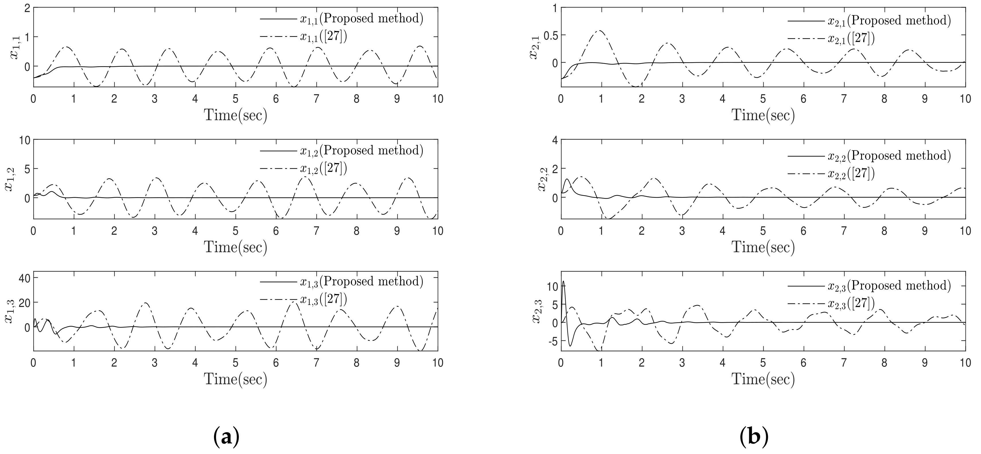
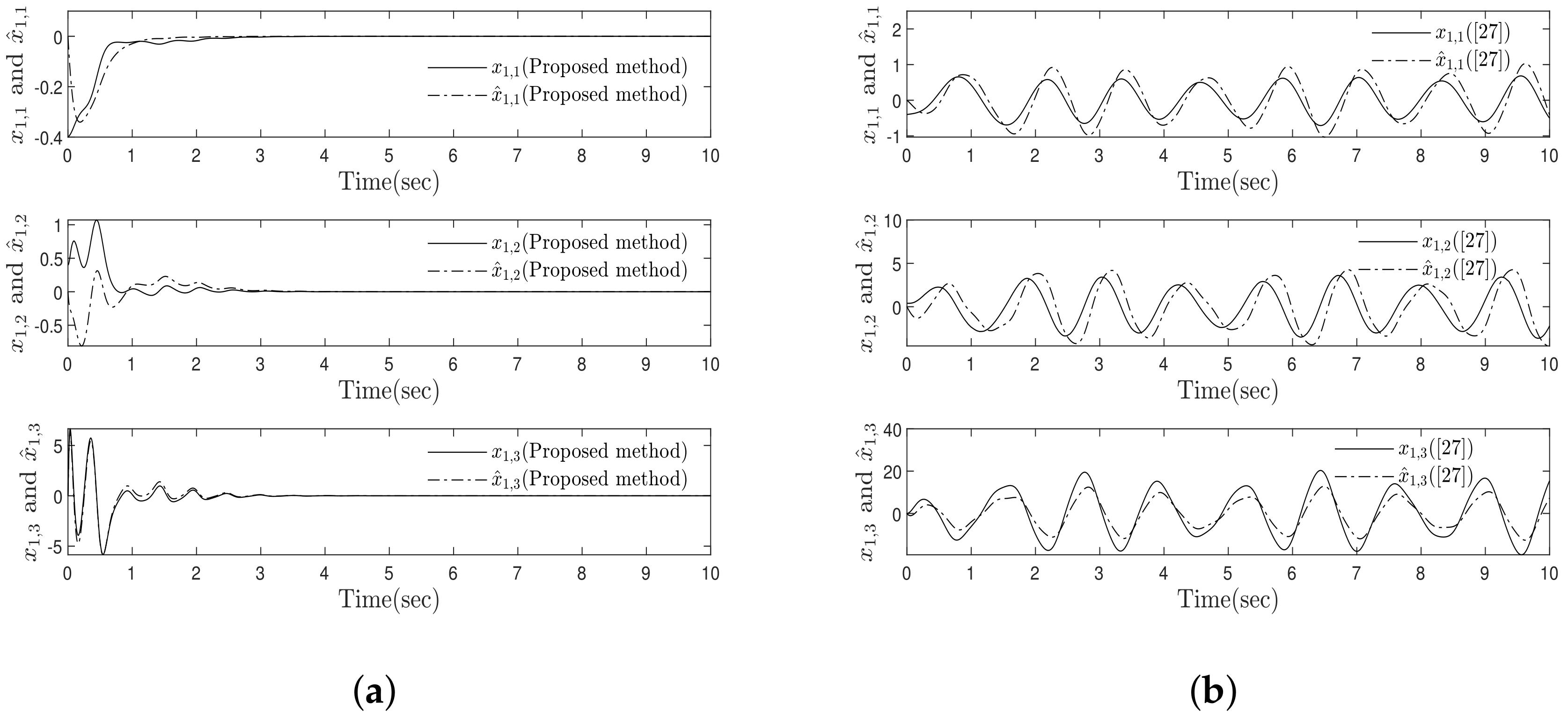
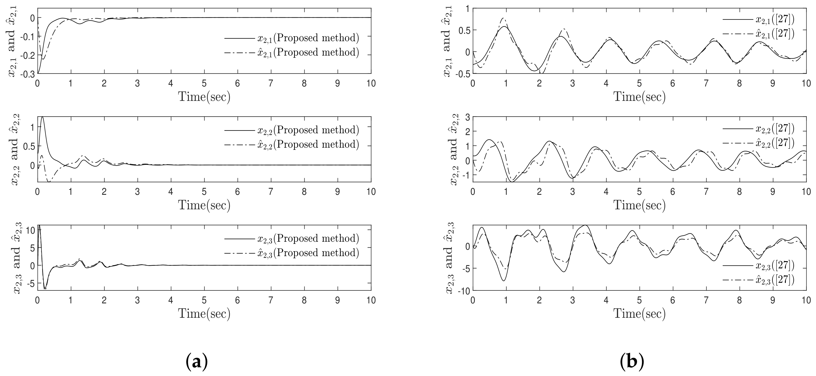
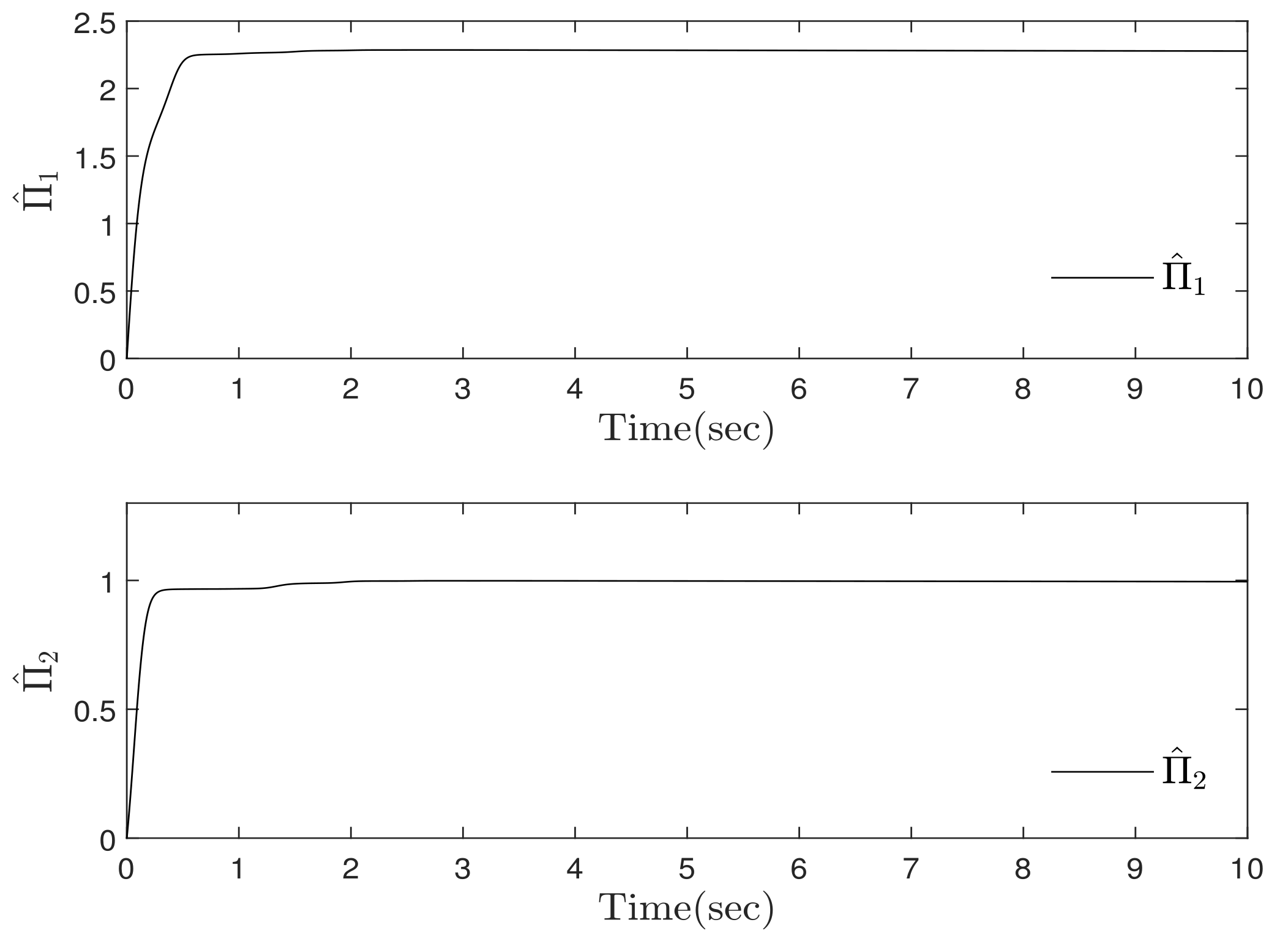
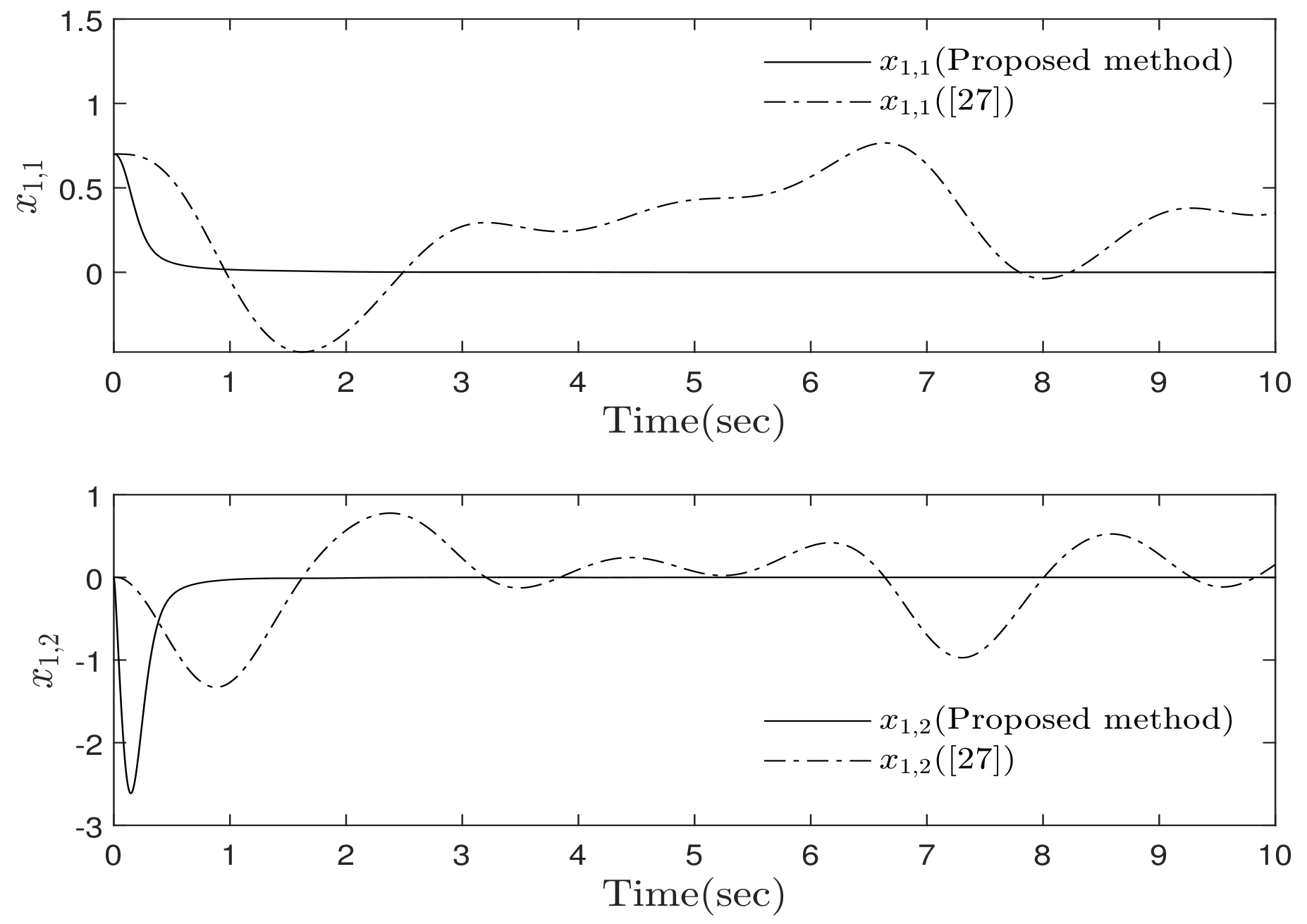
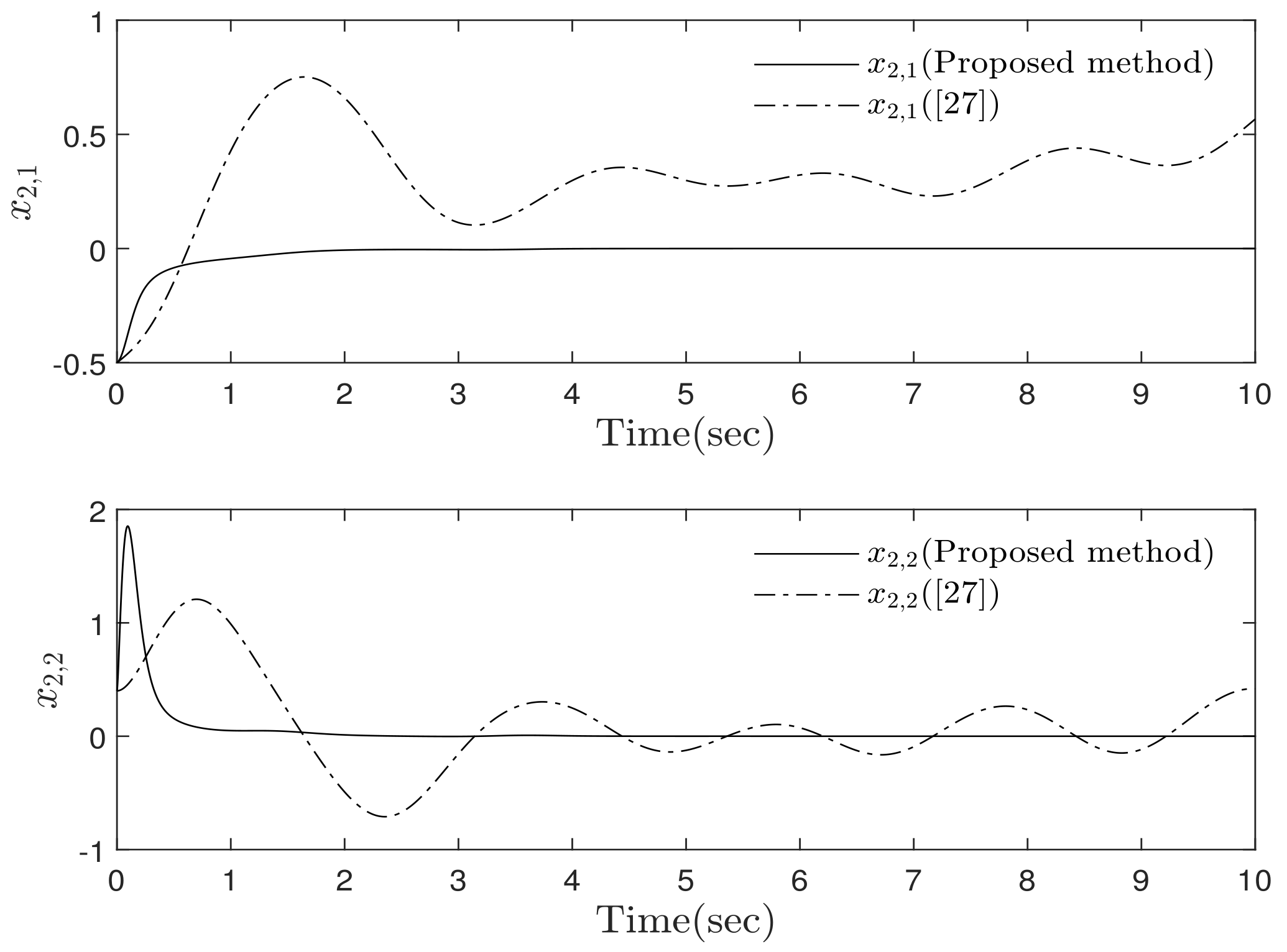
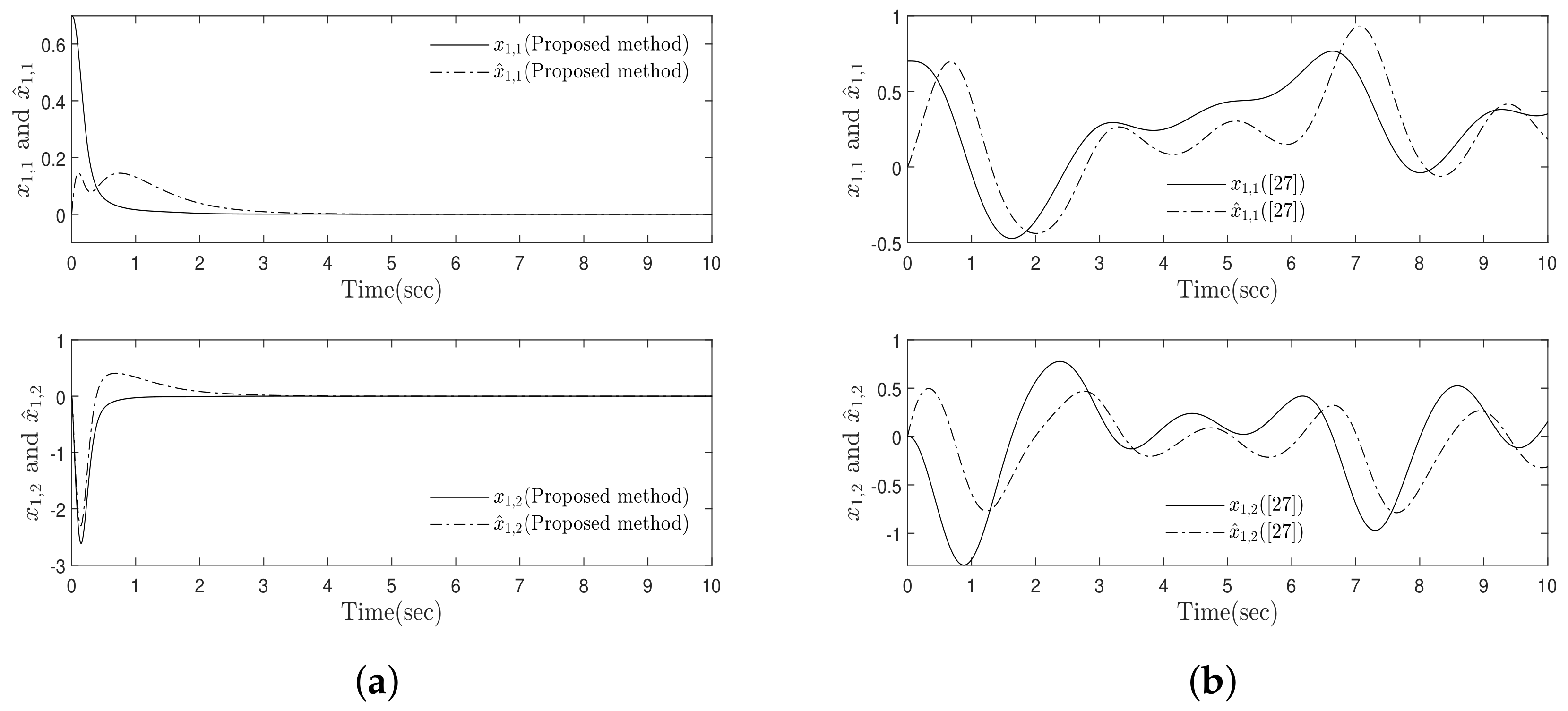
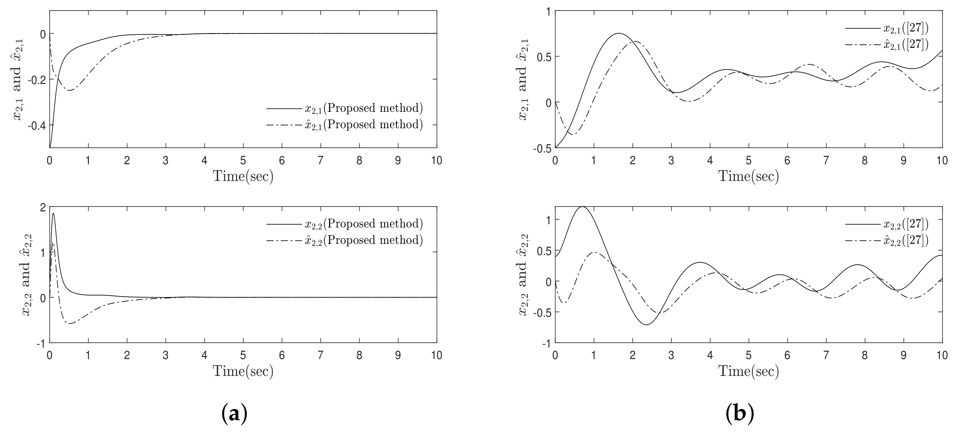
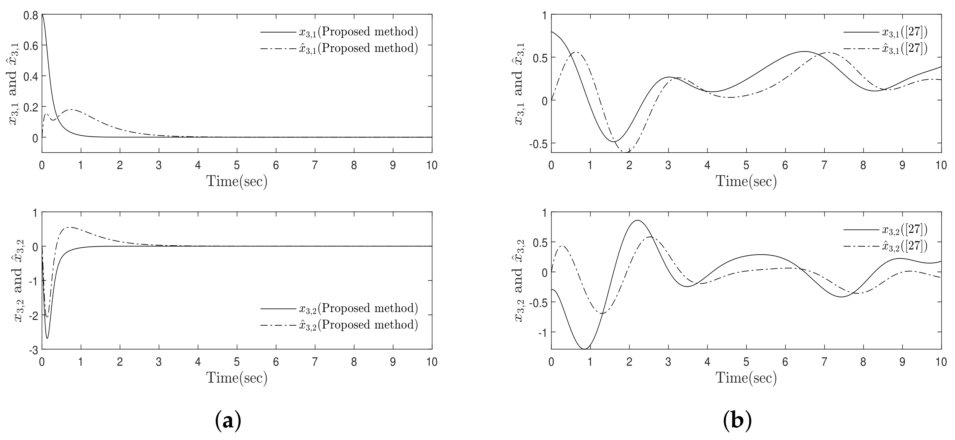
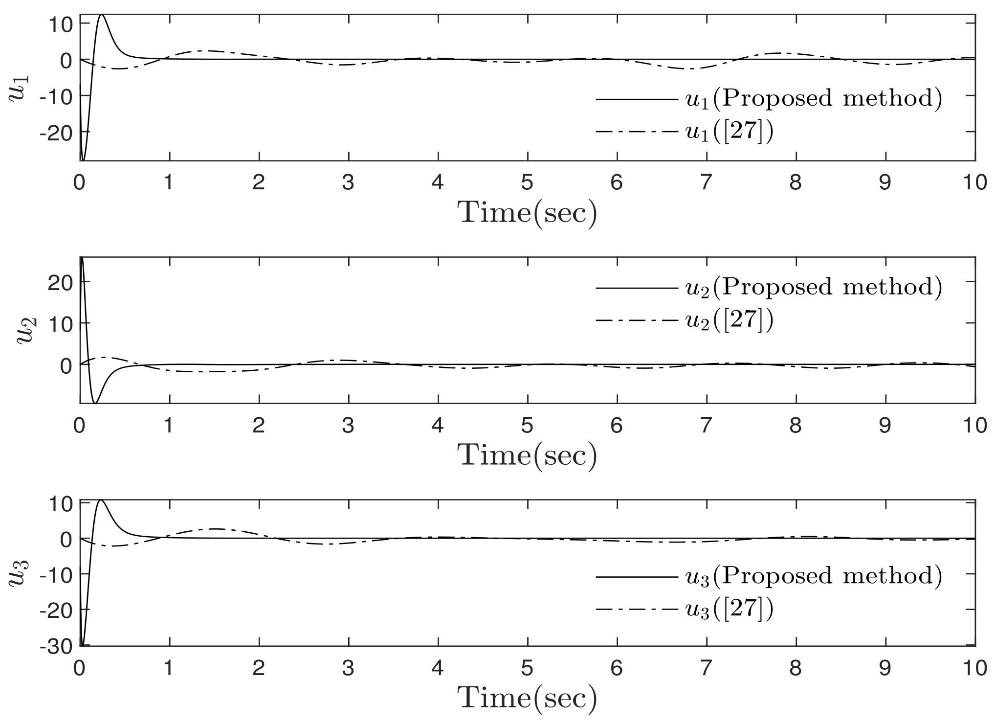
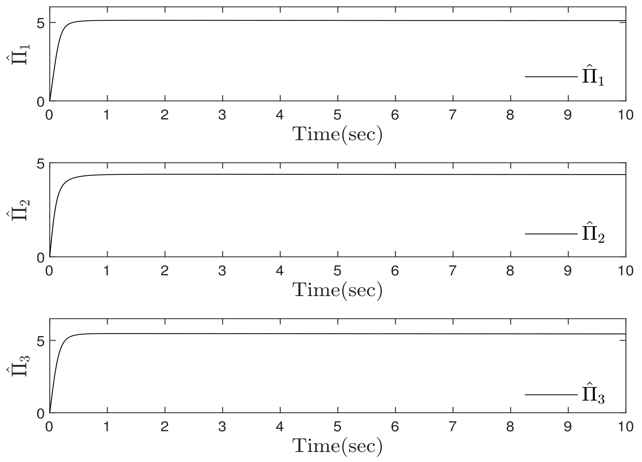
The simulation results are displayed in Figure 1, Figure 2, Figure 3, Figure 4 and Figure 5. Figure 1 compares the local stabilization results of the proposed local control system with those of the local control system of [27]. By the output-feedback corrupted by the unknown measurement sensitivities, the proposed control system can achieve robust stabilization, but the local states of the control system [27] do not stabilize. This implies that the effects of the unknown measurement sensitivities can be compensated by the proposed decentralized control approach. The state estimation results for each subsystem are shown in Figure 2 and Figure 3 where all state variables are estimated by the local observers. The local control inputs of each subsystem are compared in Figure 4. The estimated parameters of the proposed approach are displayed in Figure 5. These figures show that the proposed decentralized adaptive output-feedback control scheme ensures satisfactory stabilization performance in the presence of unknown measurement sensitivities while all signals of the closed-loop system (51)–(53) are bounded.
Example 2.
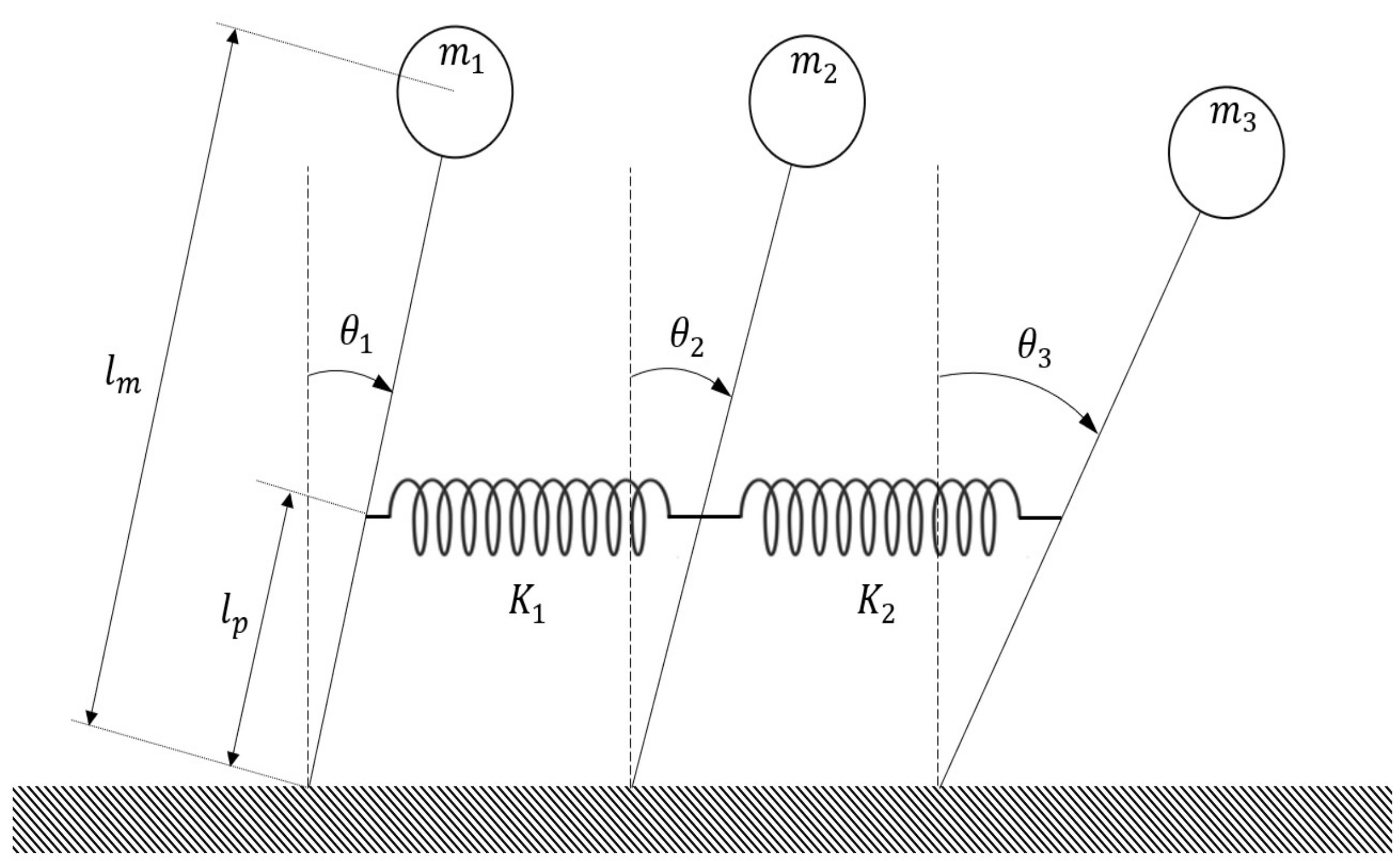
In this example, we consider the tripled inverted pendulum connected by springs, as shown in Figure 6. Because the inverted pendulum system is an inherently unstable system, one of its basic research topics is the balance and posture control. These inverted pendulum systems have been applied to various technical real-world applications such as bipedal walking robots [39], a two-wheeled vehicle [40], and an exoskeleton robot [41]. The proposed decentralized control design via the output feedback corrupted by sensor sensitivities can provide a basic research result for the practical experiments of these technical real-world applications. Thus, the mathematical model of the tripled inverted pendulum is considered as a simulation example in this paper. The motion equations of the pendulums are given by [42]:
where and are the angle and the end mass of the ith pendulum, g is the gravitational acceleration, is the length of each rod, is the distance between the pivot and the center of gravity of the rod, and are the spring constants, and is the control input torque with . The system parameters are set to kg, kg, kg, m/s, m, m, , and . By the transformation of coordinates and , the interconnected system (54) is rewritten as follows:
where , , , , and . Assumption 2 holds with , , and . The measurement sensitivities are assumed to be , , and . The local high-gain observers and local controllers of the proposed approach are given by:
and:
where , and the design parameters are chosen as , , , , , , , , and . The simulation results shown in Figure 7, Figure 8, Figure 9, Figure 10, Figure 11, Figure 12, Figure 13 and Figure 14 are obtained under the initial conditions , , , , , , , , and . Under unknown measurement sensitivities , the local stabilization results of the proposed decentralized control system and the previous decentralized control system [27] are compared in Figure 7, Figure 8 and Figure 9. While the existing decentralized stabilization method [27] cannot compensate for unknown measurement sensitivities, which leads to the unstable result of controlled state variables, the proposed decentralized control approach can achieve the robust stabilization against unknown measurement sensitivities. Figure 10, Figure 11 and Figure 12 show the local state estimation results of each subsystem. Figure 13 compares the local control inputs. Figure 14 depicts the adaptive parameters of the proposed control approach. From these figures, the stabilization of the tripled inverted pendulum systems (55) connected by springs is successfully achieved by the proposed approach in the presence of the unknown time-varying measurement sensitivities and their unknown bounds.
5. Conclusions
This article addressed the decentralized adaptive stabilization problem for a class of uncertain nonlinear interconnected systems by the output-feedback corrupted by unknown measurement sensitivities. A local adaptive control strategy was established to compensate for the effects of the unknown bounds of the measurement sensitivities. In the Lyapunov stability sense, the stability of the proposed decentralized adaptive control system was successfully analyzed. Finally, simulation comparisons were provided to show the compensation ability of the unknown measurement sensitivities of the proposed approach.
Author Contributions
Conceptualization, methodology, software, and writing, original draft preparation, D.M.J.; conceptualization, methodology, writing, review and editing, and supervision, S.J.Y. All authors read and agreed to the published version of the manuscript.
Funding
This research was supported by the Chung-Ang University Excellent Student Scholarship in 2019 and by the National Research Foundation of Korea (NRF) grant funded by the Korean government (NRF-2019R1A2C1004898).
Conflicts of Interest
The authors declare no conflict of interest.
References
- Kolovsky, M.Z. Nonlinear Dynamics of Active and Passive Systems of Vibration Protection; Springer: Berlin/Heidelberg, Germany, 1999. [Google Scholar]
- Bernstein, D.S. Sensor performance specifications. IEEE Control. Syst. Mag. 2001, 21, 9–18. [Google Scholar]
- Carr, J.J.; Brown, J.M. Introduction to Biomedical Equipment Technology; Prentice-Hall: Upper Saddle River, NJ, USA, 2001. [Google Scholar]
- Yang, G.H.; Wang, J.L.; Soh, Y.C. Reliable H∞ controller design for linear systems. Automatica 2001, 37, 717–725. [Google Scholar] [CrossRef]
- Chen, B.; Lam, J. Reliable observer-based H∞ control of uncertain state-delayed systems. Int. J. Syst. Sci. 2004, 35, 707–718. [Google Scholar] [CrossRef]
- Zhai, J.Y.; Qian, C. Global control of nonlinear systems with uncertain output function using homogeneous domination approach. Int. J. Robust Nonlinear Control. 2012, 22, 1543–1561. [Google Scholar] [CrossRef]
- Zhai, J.Y.; Ai, W.Q.; Fei, S.M. Global output feedback stabilisation for a class of uncertain non-linear systems. IET Control Theory Appl. 2013, 7, 305–313. [Google Scholar] [CrossRef]
- Xie, X.J.; Li, Z.J.; Zhang, K. Semi-global output feedback control for nonlinear systems with uncertain time-delay and output function. Int. J. Robust Nonlinear Control 2017, 27, 2549–2566. [Google Scholar] [CrossRef]
- Li, Z.J.; Xie, X.J.; Zhang, K. Output feedback stabilisation for nonlinear systems with unknown output function and control coefficients and its application. Int. J. Control 2016, 90, 1027–1036. [Google Scholar]
- Ai, W.; Zhai, J.; Fei, S. Universal adaptive regulation for a class of nonlinear systems with unknown time delays and output function via output feedback. J. Frankl. Inst. 2013, 350, 3168–3187. [Google Scholar] [CrossRef]
- Zhai, J.Y.; Du, H.B.; Fei, S.M. Global sampled-data output feedback stabilisation for a class of nonlinear systems with unknown output function. Int. J. Control 2016, 89, 469–480. [Google Scholar] [CrossRef]
- Chen, C.C.; Qian, C.; Sun, Z.Y.; Liang, Y.W. Global output feedback stabilization of a class of nonlinear systems with unknown measurement sensitivity. IEEE Trans. Autom. Control 2018, 63, 2212–2217. [Google Scholar] [CrossRef]
- Jain, S.; Khorrami, F. Decentralized adaptive output feedback design for large-scale nonlinear systems. IEEE Trans. Autom. Control. 1997, 42, 729–735. [Google Scholar] [CrossRef]
- Zhu, Y.; Pagilla, P.R. Decentralized output feedback control of a class of large-scale interconnected systems. IMA J. Math. Control Inf. 2007, 24, 57–69. [Google Scholar] [CrossRef]
- Zhai, J.; Zha, W.; Fei, S. Semi-global finite-time output feedback stabilization for a class of large-scale uncertain nonlinear systems. Commun. Nonlinear Sci. Numer. Simul. 2013, 18, 3181–3189. [Google Scholar] [CrossRef]
- Wu, H.S. Decentralized adaptive robust state feedback for uncertain large-scale interconnected systems with time delays. J. Optim. Theory Appl. 2005, 126, 439–462. [Google Scholar] [CrossRef]
- Wei, C.; Luo, J.; Dai, H.; Yin, Z.; Yuan, J. Low-complexity differentiator-based decentralized fault-tolerant control of uncertain large-scale nonlinear systems with unknown dead zone. Nonlinear Dyn. 2017, 89, 2573–2592. [Google Scholar] [CrossRef]
- Shao, S.; Yang, H.; Jiang, B. Decentralized fault tolerant control for a class of interconnected nonlinear systems. IEEE Trans. Cybern. 2018, 48, 178–186. [Google Scholar] [CrossRef]
- Krstic, M.; Kanellakopoulos, I.; Kokotovic, P. Nonlinear and Adaptive Control Design; Wiley: New York, NY, USA, 1995. [Google Scholar]
- Swaroop, D.; Hedrick, J.K.; Yip, P.P.; Gerdes, J.C. Dynamic surface control for a class of nonlinear systems. IEEE Trans. Autom. Control 2000, 45, 1893–1899. [Google Scholar] [CrossRef] [Green Version]
- Yoo, S.J.; Park, J.B. Neural-network-based decentralized adaptive control for a class of large-scale nonlinear systems with unknown time-varying delays. IEEE Trans. Syst. Man Cybern. B Cybern. 2009, 39, 1316–1322. [Google Scholar]
- Mehraeen, S.; Jagannathan, S.; Crow, M.L. Decentralized dynamic surface control of large-scale interconnected systems in strict-feedback form using neural networks with asymptotic stabilization. IEEE Trans. Neural Netw. 2011, 22, 1709–1722. [Google Scholar] [CrossRef]
- Tong, S.; Li, Y. Adaptive fuzzy decentralized output feedback control for nonlinear large-scale systems with unknown dead-zone inputs. IEEE Trans. Fuzzy Syst. 2013, 21, 913–925. [Google Scholar] [CrossRef]
- Du, P.; Liang, H.; Zhao, S.; Ahn, C.K. Neural-based decentralized adaptive finite-time control for nonlinear large-scale systems with time-varying output constraints. IEEE Trans. Syst. Man Cybern. Syst. 2019. [Google Scholar] [CrossRef]
- Zhang, X.; Lin, Y. Nonlinear decentralized control of large-scale systems with strong interconnections. Automatica 2014, 50, 2419–2423. [Google Scholar] [CrossRef]
- Li, Y.X.; Tong, S.; Yang, G.H. Observer-based adaptive fuzzy decentralized event-triggered control of interconnected nonlinear system. IEEE Trans. Cybern. 2019. [Google Scholar] [CrossRef] [PubMed]
- Frye, M.T.; Qian, C.; Colgren, R. Decentralized control of large-scale uncertain nonlinear systems by linear output feedback. Communi. Inf. Syst. 2005, 4, 191–210. [Google Scholar]
- Wang, C.; Wen, C.; Lin, Y. Decentralized adaptive backsteeping control for a class of interconnected nonlinear systems with unknown actuator failures. J. Frankl. Inst. 2015, 352, 835–850. [Google Scholar] [CrossRef]
- Choi, Y.H.; Yoo, S.J. Event-triggered decentralized adaptive fault-tolerant control of uncertina interconnected nonlinear systems with actuator failures. ISA Trans. 2018, 77, 77–89. [Google Scholar] [CrossRef]
- Wang, H.Q.; Liu, P.X.P.; Bao, J.L.; Xie, X.J.; Li, S. Adaptive neural output-feedback decentralized control for large-scale nonlinear systems with stochastic disturbances. IEEE Trans Neural Netw. Learn. Syst. 2019, 31, 972–983. [Google Scholar] [CrossRef]
- Zhang, Q.; Zhai, D.; Dong, J. Observer-based adaptive fuzzy decentralized control of uncertain large-scale nonlinear systems with full state contraints. Int. J. Fuzzy Syst. 2019, 21, 1085–1103. [Google Scholar] [CrossRef]
- Liu, T.; Jiang, Z.P.; Hill, D.J. Decentralized output-feedback control of large-scale nonlinear systems with sensor noise. Automatica 2012, 48, 2560–2568. [Google Scholar] [CrossRef]
- Qian, C.; Lin, W. Output feedback control of a class of nonlinear systems: A nonseparation principle paradigm. IEEE Trans. Autom. Control 2002, 47, 1710–1715. [Google Scholar] [CrossRef] [Green Version]
- Lei, H.; Lin, W. Universal adaptive control of nonlinear systems with unknown growth rate by output feedback. Automatica 2006, 42, 1783–1789. [Google Scholar] [CrossRef]
- Ioannou, P.A.; Kokotovic, P.V. Adaptive Systems with Reduced Models; Springer: New York, NY, USA, 1983. [Google Scholar]
- Ge, S.S.; Tee, K.P. Approximation-based control of nonlinear MIMO time-delay systems. Automatica 2007, 43, 31–43. [Google Scholar] [CrossRef] [Green Version]
- Choi, Y.H.; Yoo, S.J. Simple adaptive output-feedback control of non-linear strict-feedback time-delay systems. IET Control Theory Appl. 2016, 10, 58–66. [Google Scholar] [CrossRef]
- Jeong, D.M.; Choi, Y.H.; Yoo, S.J. Adaptive output-feedback control of a class of nonlinear systems with unknown sensor sensitivity and its experiment for flexible-joint robots. J. Electr. Eng. Technol. 2020, 15, 907–918. [Google Scholar] [CrossRef]
- Feng, S.; Sun, Z. Biped robot walking using three-mass linear inverted pendulum model. In International Conference on Intelligent Robotics and Applications; Springer: Berlin/Heidelberg, Germany, 2008; pp. 371–380. [Google Scholar]
- Takei, T.; Imamura, R. Baggage transportation and navigation by a wheeled inverted pendulum mobile robot. IEEE Trans. Ind. Electron. 2009, 56, 3985–3994. [Google Scholar] [CrossRef]
- Chen, Q.; Cheng, H.; Yue, C.; Huang, R.; Guo, H. Dynamic balance gait for walking assistance exoskeleton. Appl. Bionics Biomech. 2018, 2018, 3985–3994. [Google Scholar] [CrossRef]
- Yoo, S.J.; Park, J.B.; Choi, Y.H. Decentralized adaptive stabilization of interconnected nonlinear systems with unknown non-symmetric dead-zone inputs. Automatica 2009, 45, 436–443. [Google Scholar] [CrossRef]
Figure 1.
Comparison of the stabilization results of System (51): (a) the state variables of the first subsystem; (b) the state variables of the second subsystem.
Figure 1.
Comparison of the stabilization results of System (51): (a) the state variables of the first subsystem; (b) the state variables of the second subsystem.

Figure 2.
Comparison of the estimation results and , , for the first subsystem of System (51): (a) the proposed decentralized control scheme; (b) the decentralized control scheme [27].

Figure 3.
Comparison of the estimation results and , , for the second subsystem of System (51): (a) the proposed decentralized control scheme; (b) the decentralized control scheme [27].

Figure 4.
Comparison of control inputs , for System (51): (a) ; (b) .
Figure 4.
Comparison of control inputs , for System (51): (a) ; (b) .

Figure 5.
Parameter estimates , for System (51).
Figure 5.
Parameter estimates , for System (51).

Figure 6.
Tripled inverted pendulums connected by springs.

Figure 7.
Comparison of the stabilization results for the first subsystem of tripled inverted pendulum systems (55).
Figure 7.
Comparison of the stabilization results for the first subsystem of tripled inverted pendulum systems (55).

Figure 8.
Comparison of stabilization results for the second subsystem of tripled inverted pendulum systems (55).
Figure 8.
Comparison of stabilization results for the second subsystem of tripled inverted pendulum systems (55).

Figure 9.
Comparison of stabilization results for the third subsystem of tripled inverted pendulum systems (55).
Figure 9.
Comparison of stabilization results for the third subsystem of tripled inverted pendulum systems (55).

Figure 10.
Comparison of estimation results and , , for the first subsystem of System (55): (a) the proposed decentralized control scheme; (b) the decentralized control scheme [27].

Figure 11.
Comparison of estimation results and , , for the second subsystem of System (55): (a) the proposed decentralized control scheme; (b) the decentralized control scheme [27].

Figure 12.
Comparison of estimation results and , , for the third subsystem of System (55): (a) the proposed decentralized control scheme; (b) the decentralized control scheme [27].

Figure 13.
Comparison of control inputs , for System (55).
Figure 13.
Comparison of control inputs , for System (55).

Figure 14.
Parameter estimates , , for tripled inverted pendulum systems (55).
Figure 14.
Parameter estimates , , for tripled inverted pendulum systems (55).

© 2020 by the authors. Licensee MDPI, Basel, Switzerland. This article is an open access article distributed under the terms and conditions of the Creative Commons Attribution (CC BY) license (http://creativecommons.org/licenses/by/4.0/).
Share and Cite
MDPI and ACS Style
Jeong, D.M.; Yoo, S.J. Decentralized Adaptive Tracking of Interconnected Nonlinear Systems by Corrupted Output Feedback. Mathematics 2020, 8, 1340. https://doi.org/10.3390/math8081340
AMA Style
Jeong DM, Yoo SJ. Decentralized Adaptive Tracking of Interconnected Nonlinear Systems by Corrupted Output Feedback. Mathematics. 2020; 8(8):1340. https://doi.org/10.3390/math8081340
Chicago/Turabian StyleJeong, Dong Min, and Sung Jin Yoo. 2020. "Decentralized Adaptive Tracking of Interconnected Nonlinear Systems by Corrupted Output Feedback" Mathematics 8, no. 8: 1340. https://doi.org/10.3390/math8081340
Note that from the first issue of 2016, this journal uses article numbers instead of page numbers. See further details here.