Tracking Control Strategy Using Filter-Based Approximation for the Unknown Control Direction Problem of Uncertain Pure-Feedback Nonlinear Systems

Abstract

A filter-based recursive tracker design approach is presented for the problem of unknown control directions of pure-feedback systems with completely unknown non-affine nonlinearities. In the controller design procedure, the first-order filters for error surfaces, a control input, and state variables are employed to design nonadaptive virtual and actual control laws independent of adaptive function approximators. In addition, for the unknown control direction problem, the filtering signals are incorporated with Nussbaum functions. Different from existing adaptive approximation-based control schemes in the presence of unknown control directions, the proposed approach does not require any adaptive technique regardless of completely unknown nonlinear functions. Therefore, a simplified tracking structure can be constructed. Using the Lyapunov stability analysis, it is shown that the tracking error is reduced within an adjustable neighborhood of the origin while ensuring all the closed-loop signals are bounded.

1. Introduction

In the past few decades, the control of nonlinear systems has attracted considerable attention due to its theoretic interest and various applications [1]. Especially since systematic and recursive designs such as the backstepping technique [2] and the dynamic surface control technique [3] were developed, adaptive recursive control designs have been actively studied for several uncertain nonlinear systems in strict-feedback form [4,5,6,7,8,9,10,11,12,13,14,15,16,17,18,19,20,21,22,23] and in pure-feedback form [24,25,26,27,28,29,30,31,32,33,34,35], where pure-feedback systems have the non-affine property of state variables to be used as virtual controls. In practice, pure-feedback systems can represent the mathematical models of many engineering applications such as continuous stirred tank reactors [2], piezoelectric actuators [36], PMSM servo systems [37], rolling mills [38], hypersonic vehicles [39], and so on. Additionally, since general nonlinear systems can be converted into the systems in triangular form under some conditions [40], pure-feedback systems can be used in broad applications. Among the existing recursive control designs, the adaptive function approximation methodologies based on neural networks or fuzzy systems were utilized in [8,9,10,11,12,13,14,15,16,17,18,19,20,21,22,23,24,25,26,27,28,29,30,31,32,33,34,35] to compensate for the effects of completely unknown nonlinearities in the recursive design procedure. However, these adaptive controllers suffered from the following intrinsic features of neural networks and fuzzy approximators: (i) The high approximation accuracy is achieved when the optimal structure of basis functions and the sufficiently large number of optimal weights are chosen, but it is hard to find the optimal structure a priori because nonlinear functions are completely unknown. (ii) The large number of optimal weights leads to more differential equations, called adaptation laws, to be solved to update estimated weights. In order to overcome these restrictions, a filter-based tracking control strategy for uncertain nonlinear systems was firstly presented in [41]. The major contribution of this strategy is to replace adaptive function approximators with nonadaptive filter-based approximators where the filter-based approximator is defined as the linear combination of states, a control input, and their filtered signals. Thus, the aforementioned problems (i) and (ii) of adaptive function approximators can be overcome by the strategy of [41]. Despite these advantages of [41], the unknown control direction problem has not been solved in the filter-based control framework. Since the filter-based approximators presented in [41] should be designed by using the exact information of control directions, the existing Nussbaum function approaches in the existing adaptive function-approximation-based control designs [13,14,15,16,17,18,19,20,21,33,34,35] cannot be straightforwardly applied to the filter-based control problem in the presence of unknown control directions. Furthermore, the closed-loop stability analysis considering filtering errors and Nussbaum function technique should be newly developed in the filter-based tracking framework.

Motivated by this observation, this paper investigates a filter-based tracker design problem of uncertain pure-feedback nonlinear systems with unknown control directions. The first-order filters for error surfaces, a control input, and state variables are employed to design nonadaptive virtual and actual control laws without using adaptive neural networks or fuzzy logic systems. To consider the unknown control direction problem in the filter-based tracking framework, the difference signal between the error surface and its filtered signal that is incorporated with a Nussbaum function at each design step is used for designing virtual and actual controllers. The filter-based tracking strategy using Nussbaum functions is developed to provide a new solution to the unknown control direction problem of pure-feedback nonlinear systems with completely unknown nonlinearities. Using the Lyapunov stability theory, the semi-global uniform ultimate boundedness of the closed-loop signals and the convergence of the tracking error to an adjustable neighborhood of the origin are guaranteed.

The major contributions of the proposed theoretical approach are emphasized as follows:

(i)

Different from the existing control schemes using the adaptive function approximation technique for uncertain lower-triangular nonlinear systems with unknown control directions [13,14,15,16,17,18,19,20,21,33,34,35], we present a new nonadaptive control strategy using first-order filtered signals of error surfaces, a control input, and state variables. Therefore, the proposed control approach does not require the calculation of the differential equations for tuning adaptive parameters. Accordingly, a simplified tracking control structure is established in the presence of unknown non-affine nonlinearities and unknown control directions.

(ii)

Contrary to the previous filter-based control approach [41], the proposed control scheme can handle the unknown control direction problem in the filter-based control framework. A new design approach that incorporates Nussbaum functions and filtered signals and its stability analysis are presented.

The rest of this paper is organized as follows. In Section 2, a filter-based tracking control problem for uncertain pure-feedback systems with unknown control directions is formulated. The filter-based tracker design and the closed-loop stability analysis strategy are given in Section 3. Section 4 and Section 5 provide simulation results and some conclusions, respectively.

2. Problem Formulation

Consider the following uncertain pure-feedback systems:

$$\begin{array}{c}{\dot{x}}_k\left(t\right)=p_k({\overline{x}}_k\left(t\right),x_{k+1}\left(t\right))+d_k\left(t\right),k=1,\dots ,n-1,\hfill \\ {\dot{x}}_n\left(t\right)=p_n({\overline{x}}_n\left(t\right),u\left(t\right))+d_n\left(t\right),\hfill \end{array}$$

(1)

where $x_k\left(t\right)$ and $x_n\left(t\right)$ are state variables, ${\overline{x}}_k\left(t\right)={[x_1\left(t\right),\dots ,x_k\left(t\right)]}^{\top }\in {\mathbb{R}}^k$, ${\overline{x}}_n\left(t\right)={[x_1\left(t\right),\dots ,x_n\left(t\right)]}^{\top }\in {\mathbb{R}}^n$, $u\left(t\right)\in \mathbb{R}$ is the control input, $p_k({\overline{x}}_k\left(t\right),x_{k+1}\left(t\right)):{\mathbb{R}}^{i+1}\mapsto \mathbb{R}$ and $p_n({\overline{x}}_n\left(t\right),u\left(t\right)):{\mathbb{R}}^{n+1}\mapsto \mathbb{R}$ are unknown $C^1$ non-affine nonlinear functions, and $d_k\left(t\right)$ and $d_n\left(t\right)$ are unknown bounded time-varying disturbances. Here, n denotes the order of System (1).

Assumption 1

([23]). The reference signal $r\left(t\right)\in \mathbb{R}$ denoting the target signal is available for feedback. In addition, $r\left(t\right)$ and its time derivatives $\dot{r}\left(t\right)$ and $\ddot{r}\left(t\right)$ are bounded.

Assumption 2

([42]). Define $b_i\left({\overline{x}}_{i+1}\left(t\right)\right)=\partial p_i\left({\overline{x}}_{i+1}\left(t\right)\right)/\partial x_{i+1}\left(t\right)$ where $i=1,\dots ,n$ and $x_{n+1}\left(t\right)=u\left(t\right)$. There exist unknown constants ${\underline{b}}_i$ such that $0<{\underline{b}}_i\le \left|b_i\left({\overline{x}}_{i+1}\left(t\right)\right)\right|$. The signs of $b_i\left({\overline{x}}_{i+1}\left(t\right)\right)$ representing the control directions are unknown.

Definition 1

([43]). A function $\Theta \left(\theta \right(t\left)\right)$ is called a Nussbaum-type function if the following equalities hold:

$$\underset{h\to +\infty }{lim\; sup}\frac{1}{h}{\int }_0^h\Theta \left(\theta \left(t\right)\right)d\theta =\infty ,$$

$$\underset{h\to +\infty }{lim\; inf}\frac{1}{h}{\int }_0^h\Theta \left(\theta \left(t\right)\right)d\theta =-\infty .$$

A Nussbaum function $\Theta \left(\theta \left(t\right)\right)={\theta }^2\left(t\right)cos\left(\theta \left(t\right)\right)$ is adopted in this paper.

Problem 1.

Our problem is to design a filter-based controller $u\left(t\right)$ for System (1) in a nonadaptive framework so that the state variable $x_1\left(t\right)$ follows the reference signal $r\left(t\right)$ while all the signals in the closed-loop system are bounded.

3. Filter-Based Tracking Control Design for the Problem of Unknown Control Directions

3.1. Controller Design

In this section, we focus on the design of the filter-based control scheme for (1). A recursive control design based on the backstepping technique [2] is presented using the following coordinate transformation:

$$\begin{array}{c}{\eta }_1\left(t\right)=x_1\left(t\right)-r\left(t\right),\hfill \\ {\eta }_{k+1}\left(t\right)=x_{k+1}\left(t\right)-{\psi }_k\left(t\right),\hfill \end{array}$$

(2)

where $k=1,\dots ,n-1$, ${\eta }_1\left(t\right)$, and ${\eta }_{k+1}\left(t\right)$ are error surfaces and ${\psi }_k\left(t\right)$ are virtual control laws.

Step 1: Consider the first error ${\eta }_1\left(t\right)$. Then, its time derivative using (1) is:

$${\dot{\eta }}_1\left(t\right)=p_1(x_1\left(t\right),x_2\left(t\right))+d_1\left(t\right)-\dot{r}\left(t\right)=b_1^{*}{x}_2\left(t\right)+q_1(x_1\left(t\right),x_2\left(t\right),t)$$

(3)

where $b_1^{*}=\mathrm{sign}\left(b_1\left(t\right)\right){\underline{b}}_1$ and $q_1(x_1\left(t\right),x_2\left(t\right),t)=p_1(x_1\left(t\right),x_2\left(t\right))-b_1^{*}{x}_2\left(t\right)+d_1\left(t\right)-\dot{r}\left(t\right)$. For notation conciseness, $q_1(x_1\left(t\right),x_2\left(t\right),t)$ will be described as $q_1\left(t\right)$. By rearranging (3), we have:

$$q_1\left(t\right)={\dot{\eta }}_1\left(t\right)-b_1^{*}{x}_2\left(t\right).$$

Then, the filtered signal $q_{1,f}\left(t\right)$ of $q_1\left(t\right)$ is obtained as:

$$q_{1,f}\left(t\right)={\dot{\eta }}_{1,f}\left(t\right)-b_1^{*}{x}_{2,f}\left(t\right)$$

(4)

where ${\eta }_{1,f}\left(t\right)$ and $x_{2,f}\left(t\right)$ are signals provided by the first-order low-pass filters as follows:

$${\tau }_1{\dot{\eta }}_{1,f}\left(t\right)+{\eta }_{1,f}\left(t\right)={\eta }_1\left(t\right),{\eta }_{1,f}\left(0\right)={\eta }_1\left(0\right),$$

(5)

$${\tau }_1{\dot{x}}_{2,f}\left(t\right)+x_{2,f}\left(t\right)=x_2\left(t\right),x_{2,f}\left(0\right)=x_2\left(0\right),$$

(6)

where ${\tau }_1>0$ is the small time constant of the filters. Using (5), it holds that ${\dot{\eta }}_{1,f}\left(t\right)=({\eta }_1\left(t\right)-{\eta }_{1,f}\left(t\right))/{\tau }_1$. Then, (4) becomes:

$$q_{1,f}\left(t\right)=\frac{{\eta }_1\left(t\right)-{\eta }_{1,f}\left(t\right)}{{\tau }_1}-b_1^{*}{x}_{2,f}\left(t\right).$$

(7)

From (2) and (7), ${\dot{\eta }}_1\left(t\right)$ is represented by:

$${\dot{\eta }}_1\left(t\right)=b_1^{*}({\eta }_2\left(t\right)+{\psi }_1\left(t\right))+q_{1,f}\left(t\right)+{\tilde{q}}_1\left(t\right)=b_1^{*}({\eta }_2\left(t\right)+{\psi }_1\left(t\right)-x_{2,f}\left(t\right))+\frac{{\tilde{\eta }}_1\left(t\right)}{{\tau }_1}+{\tilde{q}}_1\left(t\right)$$

(8)

where ${\tilde{\eta }}_1\left(t\right)={\eta }_1\left(t\right)-{\eta }_{1,f}\left(t\right)$ and ${\tilde{q}}_1\left(t\right)=q_1\left(t\right)-q_{1,f}\left(t\right)$.

We choose a virtual control law ${\psi }_1\left(t\right)$ as:

$$\begin{array}{cc}\hfill {\psi }_1\left(t\right)& =x_{2,f}\left(t\right)+\Theta \left({\theta }_1\left(t\right)\right)\left({\gamma }_1{\eta }_1\left(t\right)+\frac{{\tilde{\eta }}_1\left(t\right)}{{\tau }_1}\right),\hfill \end{array}$$

(9)

$$\begin{array}{cc}\hfill {\dot{\theta }}_1\left(t\right)& ={\gamma }_1{\eta }_1^2\left(t\right)+\frac{{\eta }_1\left(t\right){\tilde{\eta }}_1\left(t\right)}{{\tau }_1},\hfill \end{array}$$

(10)

where ${\gamma }_1>0$ is the control gain and ${\theta }_1\left(0\right)=0$. Applying (9) to (8) gives:

$${\dot{\eta }}_1\left(t\right)=b_1^{*}{\eta }_2\left(t\right)+b_1^{*}\Theta \left({\theta }_1\left(t\right)\right)\left({\gamma }_1{\eta }_1\left(t\right)+\frac{{\tilde{\eta }}_1\left(t\right)}{{\tau }_1}\right)+\frac{{\tilde{\eta }}_1\left(t\right)}{{\tau }_1}+{\tilde{q}}_1\left(t\right).$$

(11)

A Lyapunov function candidate $V_1\left(t\right)=(1/2){\eta }_1^2\left(t\right)$ is considered. Using (10) and (11), the time derivative of $V_1\left(t\right)$ is:

$$\begin{array}{cc}{\dot{V}}_1\left(t\right)\hfill & ={\eta }_1\left(t\right)b_1^{*}{\eta }_2\left(t\right)+b_1^{*}\Theta \left({\theta }_1\left(t\right)\right){\eta }_1\left(t\right)\left({\gamma }_1{\eta }_1\left(t\right)+\frac{{\tilde{\eta }}_1\left(t\right)}{{\tau }_1}\right)+\frac{{\eta }_1\left(t\right){\tilde{\eta }}_1\left(t\right)}{{\tau }_1}+{\eta }_1\left(t\right){\tilde{q}}_1\left(t\right)\hfill \\ \hfill & ={\eta }_1\left(t\right)b_1^{*}{\eta }_2\left(t\right)+(b_1^{*}\Theta \left({\theta }_1\left(t\right)\right)+1){\dot{\theta }}_1\left(t\right)-{\gamma }_1{\eta }_1^2\left(t\right)+{\eta }_1\left(t\right){\tilde{q}}_1\left(t\right).\hfill \end{array}$$

(12)

Remark 1.

In the existing adaptive approximation-based control schemes [8,9,10,11,12,13,14,15,16,17,18,19,20,21,22,23,24,25,26,27,28,29,30,31,32,33,34,35], an unknown nonlinearity is approximated by a neural network or fuzzy logic system. For example, an unknown nonlinear function q is represented by $q=W^{*\top }S+\epsilon$ where $W^{*}$ is an optimal weight vector, S is a basis function vector, and ε is a reconstruction error. However, since $W^{*}$ is unknown, a variable $\widehat{W}$ is employed to estimate $W^{*}$ and is updated on-line along a first-order differential equation called an adaptation law. Then, an estimated nonlinear function $\widehat{q}={\widehat{W}}^{\top }S$ is defined and used to compensate for q. In contrast, the proposed approach employs a filter-based function approximator $q_f$ defined as the linear combination of the filtered signals of the state variables and the control input. Even though the structure of $q_f$ is non-adaptive, its approximation ability is rigorously analyzed in the proof of Theorem 1.

Step j ($j=2,\dots ,n-1$): The time derivative of ${\eta }_j\left(t\right)$ is given by:

$${\dot{\eta }}_j\left(t\right)=p_j({\overline{x}}_j\left(t\right),x_{j+1}\left(t\right))+d_j\left(t\right)-{\dot{\psi }}_{j-1}\left(t\right)=b_j^{*}{x}_{j+1}\left(t\right)+q_j({\overline{x}}_j\left(t\right),x_{j+1}\left(t\right),t)$$

(13)

where $b_j^{*}=\mathrm{sign}\left(b_j\left(t\right)\right){\underline{b}}_j$ and $q_j({\overline{x}}_j\left(t\right),x_{j+1}\left(t\right),t)=p_j({\overline{x}}_j\left(t\right),x_{j+1}\left(t\right))-b_j^{*}{x}_{j+1}\left(t\right)+d_j\left(t\right)-{\dot{\psi }}_{j-1}\left(t\right)$. For notation conciseness, $q_j({\overline{x}}_j\left(t\right),x_{j+1}\left(t\right),t)$ will be described as $q_j\left(t\right)$.

Then, $q_j\left(t\right)$ can be rewritten as:

$$q_j\left(t\right)={\dot{\eta }}_j\left(t\right)-b_j^{*}{x}_{j+1}\left(t\right).$$

The filtered signal $q_{j,f}\left(t\right)$ of $q_j\left(t\right)$ is given by:

$$q_{j,f}\left(t\right)={\dot{\eta }}_{j,f}\left(t\right)-b_j^{*}{x}_{j+1,f}\left(t\right)$$

where ${\eta }_{j,f}\left(t\right)$ and $x_{j+1,f}\left(t\right)$ are output signals of the first-order filters:

$${\tau }_j{\dot{\eta }}_{j,f}\left(t\right)+{\eta }_{j,f}\left(t\right)={\eta }_j\left(t\right),{\eta }_{j,f}\left(0\right)={\eta }_j\left(0\right),$$

(14)

$${\tau }_j{\dot{x}}_{j+1,f}\left(t\right)+x_{j+1,f}\left(t\right)=x_{j+1}\left(t\right),x_{j+1,f}\left(0\right)=x_{j+1}\left(0\right),$$

(15)

where ${\tau }_j>0$ is the small time constant.

Using (14), we can define $q_{j,f}\left(t\right)$ as follows:

$$q_{j,f}\left(t\right)=\frac{{\eta }_j\left(t\right)-{\eta }_{j,f}\left(t\right)}{{\tau }_j}-b_j^{*}{x}_{j+1,f}\left(t\right).$$

(16)

Using (2) and (16), we have:

$${\dot{\eta }}_j\left(t\right)=b_j^{*}({\eta }_{j+1}\left(t\right)+{\psi }_j\left(t\right)-x_{j+1,f}\left(t\right))+\frac{{\tilde{\eta }}_j\left(t\right)}{{\tau }_j}+{\tilde{q}}_j\left(t\right)$$

where ${\tilde{\eta }}_j\left(t\right)={\eta }_j\left(t\right)-{\eta }_{j,f}\left(t\right)$ and ${\tilde{q}}_j\left(t\right)=q_j\left(t\right)-q_{j,f}\left(t\right)$.

Then, a virtual control law ${\psi }_j\left(t\right)$ is chosen as:

$${\psi }_j\left(t\right)=x_{j+1,f}\left(t\right)+\Theta \left({\theta }_j\left(t\right)\right)\left({\gamma }_j{\eta }_j\left(t\right)+\frac{{\tilde{\eta }}_j\left(t\right)}{{\tau }_j}+{\delta }_j{\eta }_{j-1}^2\left(t\right){\eta }_j\left(t\right)\right),$$

(17)

$${\dot{\theta }}_j\left(t\right)={\gamma }_j{\eta }_j^2\left(t\right)+\frac{{\eta }_j\left(t\right){\tilde{\eta }}_j\left(t\right)}{{\tau }_j}+{\delta }_j{\eta }_{j-1}^2\left(t\right){\eta }_j^2\left(t\right),$$

(18)

where ${\gamma }_j>0$ is the control gain, ${\delta }_j>0$ is a design parameter, and ${\theta }_j\left(0\right)=0$. From (2) and (17), ${\dot{\eta }}_j\left(t\right)$ becomes:

$${\dot{\eta }}_j\left(t\right)=b_j^{*}{\eta }_{j+1}\left(t\right)+b_j^{*}\Theta \left({\theta }_j\left(t\right)\right)\left({\gamma }_j{\eta }_j\left(t\right)+\frac{{\tilde{\eta }}_j\left(t\right)}{{\tau }_j}+{\delta }_j{\eta }_{j-1}^2\left(t\right){\eta }_j\left(t\right)\right)+\frac{{\tilde{\eta }}_j\left(t\right)}{{\tau }_j}+{\tilde{q}}_j\left(t\right).$$

(19)

A Lyapunov function candidate $V_j\left(t\right)=(1/2){\eta }_j^2\left(t\right)$ is considered. Then, ${\dot{V}}_j\left(t\right)$ becomes:

$${\dot{V}}_j\left(t\right)={\eta }_j\left(t\right)b_j^{*}{\eta }_{j+1}\left(t\right)+(b_j^{*}\Theta \left({\theta }_j\left(t\right)\right)+1){\dot{\theta }}_j\left(t\right)-{\delta }_j{\eta }_{j-1}^2\left(t\right){\eta }_j^2\left(t\right)-{\gamma }_j{\eta }_j^2\left(t\right)+{\eta }_j\left(t\right){\tilde{q}}_j\left(t\right).$$

(20)

Step n: The time derivative of ${\eta }_n\left(t\right)$ is:

$${\dot{\eta }}_n\left(t\right)=b_n^{*}u\left(t\right)+d_n\left(t\right)+q_n({\overline{x}}_n\left(t\right),u\left(t\right),t)$$

where $b_n^{*}=\mathrm{sign}\left(b_n\left(t\right)\right){\underline{b}}_n$ and $q_n({\overline{x}}_n\left(t\right),u\left(t\right),t)=p_n({\overline{x}}_n\left(t\right),u\left(t\right))-b_n^{*}u\left(t\right)+d_n\left(t\right)-{\dot{\psi }}_{n-1}\left(t\right)$. For notation conciseness, $q_n({\overline{x}}_n\left(t\right),u\left(t\right),t)$ will be described as $q_n\left(t\right)$.

Proceeding similarly, we can define a filtered signal $q_{n,f}\left(t\right)$ of $q_n\left(t\right)$ as follows:

$$q_{n,f}\left(t\right)=\frac{{\eta }_n\left(t\right)-{\eta }_{n,f}\left(t\right)}{{\tau }_n}-b_n^{*}{u}_f\left(t\right)$$

(21)

where ${\tau }_n>0$ is the small time constant and ${\eta }_{n,f}\left(t\right)$ and $u_f\left(t\right)$ are signals provided by the following filters:

$${\tau }_n{\dot{\eta }}_{n,f}\left(t\right)+{\eta }_{n,f}\left(t\right)={\eta }_n\left(t\right),{\eta }_{n,f}\left(0\right)={\eta }_n\left(0\right),$$

(22)

$${\tau }_n{\dot{u}}_f\left(t\right)+u_f\left(t\right)=u\left(t\right),u_f\left(0\right)=u\left(0\right).$$

(23)

An actual control law $u\left(t\right)$ is chosen as:

$$u\left(t\right)=u_f\left(t\right)+\Theta \left({\theta }_n\left(t\right)\right)\left({\gamma }_n{\eta }_n\left(t\right)+\frac{{\tilde{\eta }}_n\left(t\right)}{{\tau }_n}+{\delta }_n{\eta }_{n-1}^2\left(t\right){\eta }_n\left(t\right)\right),$$

(24)

$${\dot{\theta }}_n\left(t\right)={\gamma }_n{\eta }_n^2\left(t\right)+\frac{{\eta }_n\left(t\right){\tilde{\eta }}_n\left(t\right)}{{\tau }_n}+{\delta }_n{\eta }_{n-1}^2\left(t\right){\eta }_n^2\left(t\right),$$

(25)

where ${\tilde{\eta }}_n\left(t\right)={\eta }_n\left(t\right)-{\eta }_{n,f}\left(t\right)$, ${\gamma }_n$ and ${\delta }_n$ are positive design parameters, and ${\theta }_n\left(0\right)=0$.

A Lyapunov function candidate $V_n\left(t\right)=(1/2){\eta }_n^2\left(t\right)$ is considered. Then, applying (24), ${\dot{V}}_n\left(t\right)$ becomes:

$${\dot{V}}_n\left(t\right)=(b_n^{*}\Theta \left({\theta }_n\left(t\right)\right)+1){\dot{\theta }}_n\left(t\right)-{\gamma }_n{\eta }_n^2\left(t\right)-{\delta }_n{\eta }_{n-1}^2\left(t\right){\eta }_n^2\left(t\right)+{\eta }_n\left(t\right){\tilde{q}}_n\left(t\right)$$

(26)

where ${\tilde{q}}_n\left(t\right)=q_n\left(t\right)-q_{n,f}\left(t\right)$.

Remark 2.

The proposed filter-based controller includes the virtual and actual controllers (9), (17), and (24) with the first-order filters (5), (6), (14), (15), (22), and (23). Contrary to the previous controllers based on the adaptive function approximation for lower-triangular nonlinear systems with unknown control directions [13,14,15,16,17,18,19,20,21,33,34,35], the proposed tracking system does not use any adaptive function approximators using neural networks or fuzzy systems. For the detailed comparison, the neural network-based control scheme reported in [33] is given as follows:

$$\begin{array}{c}{\psi }_k\left(t\right)=\Theta \left({\theta }_k\left(t\right)\right)[{\gamma }_k{z}_k\left(t\right)+{\widehat{W}}_k^{\top }\left(t\right)S_k\left({\nu }_k\left(t\right)\right)],\hfill \\ u\left(t\right)=\Theta \left({\theta }_n\left(t\right)\right)[{\gamma }_n{z}_n\left(t\right)+{\widehat{W}}_n^{\top }\left(t\right)S_n\left({\nu }_n\left(t\right)\right)],\hfill \\ {\dot{\theta }}_i\left(t\right)={\gamma }_i{z}_i^2\left(t\right)+z_i\left(t\right){\widehat{W}}_i^{\top }\left(t\right)S_i\left({\nu }_i\left(t\right)\right),\hfill \\ {\dot{\widehat{W}}}_i\left(t\right)={\Gamma }_i[S_i\left({\nu }_i\left(t\right)\right)z_i\left(t\right)-{\sigma }_i{\widehat{W}}_i\left(t\right)],\hfill \end{array}$$

(27)

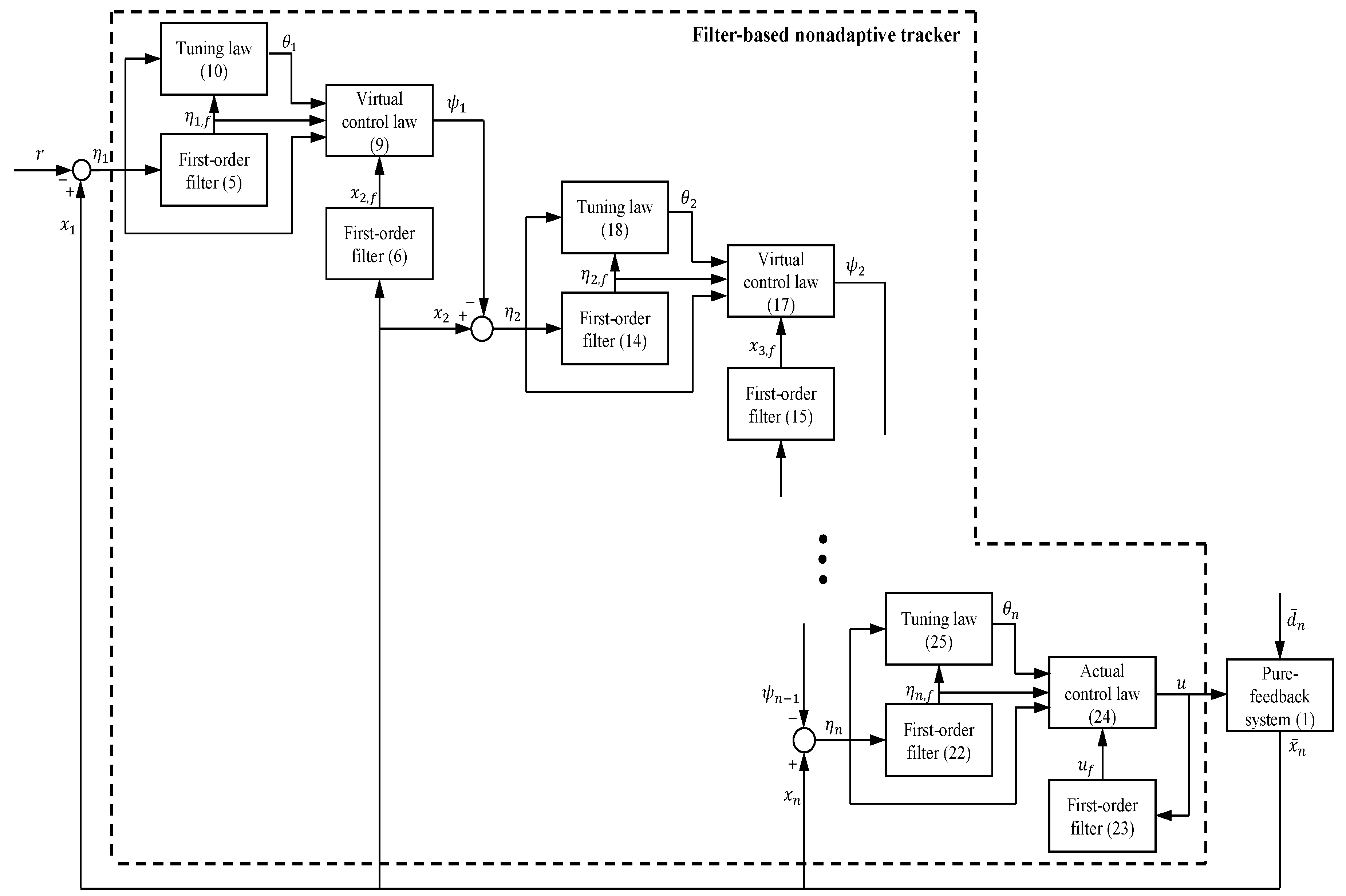
where $k=1,\dots ,n-1$, $i=1,\dots ,n$, $z_1\left(t\right)=x_1\left(t\right)-r\left(t\right)$ and $z_{k+1}\left(t\right)=x_{k+1}\left(t\right)-{\psi }_k\left(t\right)$ are error surfaces, ${\psi }_k\left(t\right)$ are the virtual control laws, $\Theta \left({\theta }_i\left(t\right)\right)$ are Nussbaum functions, ${\gamma }_i$ and ${\sigma }_i$ are positive design parameters, ${\Gamma }_i$ are positive definite matrices denoting the adaptation gains, and ${\widehat{W}}_i\left(t\right)$ and $S_i\left({\nu }_i\left(t\right)\right)$ are the estimated weighting vectors and the nonlinear basis function vectors, respectively, of the employed adaptive function approximators. In (27), it should be stressed that multiple neural networks ${\widehat{W}}_i^{\top }\left(t\right)S_i\left({\nu }_i\left(t\right)\right)$ are required to implement $u\left(t\right)$. Thus, the adaptation law to update ${\widehat{W}}_i\left(t\right)$ should be solved numerically, which can increase the computational complexity of $u\left(t\right)$. On the contrary, the proposed controller is nonadaptive as illustrated in Figure 1 where the tuning law blocks are used to update the parameters of Nussbaum functions. Accordingly, the proposed tracking system has a simpler structure than existing adaptive controllers [13,14,15,16,17,18,19,20,33,34,35]. The simple control structure is significant for the implementation of the control algorithm in the real-world embedded system. Because the embedded board is subject to the limited computational resources, it is difficult to implement complex control algorithms in one sampling time. Especially, when multi-thread programming is used to do other tasks (e.g., network communication with other embedded boards or sensors), the complex computation of the control law may provide the operating delay of the whole process. Owing to the simplicity of the proposed algorithm, the computational burden of the embedded control system for implementing the proposed control algorithm in practical applications can be reduced. This helps to reduce the operating delay of the embedded control system.

Remark 3.

In the previous filter-based control design methodology [41], the control directions were assumed to be known and positive. Then, the filter-based function approximators were designed as $g_{i,f}\left(t\right)=(x_i\left(t\right)-x_{i,f}\left(t\right))/{\tau }_0-x_{i+1,f}\left(t\right)$ in the virtual and actual control laws where $i=1,\dots ,n$, $x_{n+1,f}\left(t\right)=u_f\left(t\right)$, and ${\tau }_0$ is a time constant. However, the term $-x_{i+1,f}\left(t\right)$ in $g_{i,f}\left(t\right)$ was derived based on known signs of control coefficients. That is, the filter-based approximator $g_{i,f}\left(t\right)$ depends on the exact information of the control directions. Thus, the existing adaptive approximation-based control studies using Nussbaum functions [13,14,15,16,17,18,19,20,33,34,35] cannot be straightforwardly applied to the unknown control direction problem in the filter-based control design. Thus, we incorporate the difference signals ${\tilde{\eta }}_i\left(t\right)$, $i=1,\dots ,n$, between the error surfaces and their filtered signals with Nussbaum functions in the controller design procedure and design the term ${\delta }_{k+1}{\eta }_k^2\left(t\right){\eta }_{k+1}\left(t\right)$, $k=1,\dots ,n-1$, in (17) and (24). In this way, the unknown control direction problem can be solved in the filter-based nonadaptive control framework.

3.2. Stability Analysis

In this section, the closed-loop stability is analyzed for the proposed filter-based controller. For notation conciseness, we omit the time variable t in all signals used in Section 3.1. From the coordinate transformation (2) and the virtual control laws (9) and (17), the state variables $x_i$, $i=1,\dots ,n$, can be represented by:

$$\begin{array}{c}{x}_1({\eta }_1,r)={\eta }_1+r,\hfill \\ x_2({\eta }_1,{\eta }_2,{\theta }_1,{\eta }_{1,f},x_{2,f})={\eta }_2+{\psi }_1({\eta }_1,{\theta }_1,{\eta }_{1,f},x_{2,f}),\hfill \\ x_{j+1}({\eta }_{j-1},{\eta }_j,{\eta }_{j+1},{\theta }_j,{\eta }_{j,f},x_{j+1,f})={\eta }_{j+1}+{\psi }_j({\eta }_{j-1},{\eta }_j,{\theta }_j,{\eta }_{j,f},x_{j+1,f}),\hfill \end{array}$$

(28)

where $j=2,\dots ,n-1$. Then, using (28), the unknown non-affine nonlinear functions $q_i$, $i=1,\dots ,n$, are defined as follows:

$$\begin{array}{c}{q}_1({\overline{\eta }}_2,{\theta }_1,{\eta }_{1,f},x_{2,f},d_1,r,\dot{r})=p_1(x_1,x_2)-b_1^{*}{x}_2+d_1-\dot{r},\hfill \\ q_2({\overline{\eta }}_3,{\overline{\theta }}_2,{\overline{\eta }}_{2,f},{\overline{x}}_{3,f},{\tilde{q}}_1,{\overline{d}}_2,r)=p_2({\overline{x}}_2,x_3)-b_2^{*}{x}_3+d_2-{\dot{\psi }}_1({\overline{\eta }}_2,{\overline{x}}_2,{\theta }_1,{\eta }_{1,f},x_{2,f},{\tilde{q}}_1),\hfill \\ q_j({\overline{\eta }}_{j+1},{\overline{\theta }}_j,{\overline{\eta }}_{j,f},{\overline{x}}_{j+1,f},{\tilde{q}}_{j-2},{\tilde{q}}_{j-1},{\overline{d}}_j,r)=p_j({\overline{x}}_j,x_{j+1})-b_j^{*}{x}_{j+1}+d_j\hfill \\ -{\dot{\psi }}_{j-1}({\overline{\eta }}_j,{\overline{x}}_j,{\theta }_{j-1},{\eta }_{j-1,f},x_{j,f},{\tilde{q}}_{j-1}),j=3,\dots ,n-1\hfill \\ q_n({\overline{\eta }}_n,{\overline{\theta }}_n,{\overline{\eta }}_{n,f},{\overline{x}}_{n+1,f},{\tilde{q}}_{n-2},{\tilde{q}}_{n-1},{\overline{d}}_n,r)=p_n({\overline{x}}_n,u)-b_n^{*}u+d_n\hfill \\ -{\dot{\psi }}_{n-1}({\overline{\eta }}_n,{\overline{x}}_n,{\theta }_{n-1},{\eta }_{n-1,f},x_{n,f},{\tilde{q}}_{n-1}),\hfill \end{array}$$

(29)

where, for $i=1,\dots ,n$, ${\overline{\eta }}_i={[{\eta }_1,\dots ,{\eta }_i]}^{\top }$, ${\overline{\theta }}_i=[{\theta }_1,\dots ,$${\theta }_i{]}^{\top }$, ${\overline{\eta }}_{i,f}={[{\eta }_{1,f},\dots ,{\eta }_{i,f}]}^{\top }$, ${\overline{x}}_{i+1,f}={[x_{2,f},\dots ,x_{i+1,f}]}^{\top }$; $x_{n+1,f}$$=u_f$, ${\overline{d}}_i={[d_1,\dots ,d_i]}^{\top }$, and:

$$\begin{array}{cc}\hfill {\dot{\psi }}_1& ={\dot{x}}_{2,f}+\frac{\partial \Theta \left({\theta }_1\right)}{\partial {\theta }_1}{\dot{\theta }}_1({\gamma }_1{\eta }_1+\frac{{\tilde{\eta }}_1}{{\tau }_1})+\Theta \left({\theta }_1\right)({\gamma }_1{\dot{\eta }}_1+\frac{{\dot{\tilde{\eta }}}_1}{{\tau }_1}),\hfill \\ \hfill {\dot{\psi }}_l& ={\dot{x}}_{l+1,f}+\frac{\partial \Theta \left({\theta }_l\right)}{\partial {\theta }_l}{\dot{\theta }}_l({\gamma }_l{\eta }_l+\frac{{\tilde{\eta }}_l}{{\tau }_l}+{\delta }_l{\eta }_{l-1}^2{\eta }_l)+\Theta \left({\theta }_l\right)({\gamma }_l{\dot{\eta }}_l+\frac{{\dot{\tilde{\eta }}}_l}{{\tau }_l}+2{\delta }_l{\eta }_{l-1}{\dot{\eta }}_{l-1}{\eta }_l+{\delta }_l{\eta }_{l-1}^2{\dot{\eta }}_l)\hfill \end{array}$$

with $l=2,\dots ,n-1$.

From (29), the dynamic equations of the filtering errors ${\tilde{q}}_i$ are obtained as:

$$\begin{array}{c}{\dot{\tilde{q}}}_1=-\frac{{\tilde{q}}_1}{{\tau }_1}+{\Xi }_1({\overline{\eta }}_3,{\overline{\theta }}_2,{\overline{\eta }}_{2,f},x_{2,f},{\overline{\tilde{q}}}_2,{\overline{d}}_2,{\dot{d}}_1,\overline{\ddot{r}}),\hfill \\ {\dot{\tilde{q}}}_j=-\frac{{\tilde{q}}_j}{{\tau }_j}+{\Xi }_j({\overline{\eta }}_{j+2},{\overline{\theta }}_{j+1},{\overline{\eta }}_{j+1,f},{\overline{x}}_{j+1,f},{\overline{\tilde{q}}}_{j+1},{\dot{q}}_j,{\overline{d}}_{j+1},\overline{\ddot{r}}),\hfill \\ {\dot{\tilde{q}}}_n=-\frac{{\tilde{q}}_n}{{\tau }_n}+{\Xi }_n({\overline{\eta }}_n,{\overline{\theta }}_n,{\overline{\eta }}_{n,f},{\overline{x}}_{n+1,f},{\overline{\tilde{q}}}_n,{\overline{d}}_n,{\dot{d}}_{n-1},\overline{\ddot{r}}),\hfill \end{array}$$

(30)

where $j=2,\dots ,n-1$, ${\overline{\tilde{q}}}_i={[{\tilde{q}}_1,\dots ,{\tilde{q}}_i]}^{\top }$; $i=1,\dots ,n$, $\overline{\ddot{r}}={[r,\dot{r},\ddot{r}]}^{\top }$, and:

$$\begin{array}{cc}\hfill {\Xi }_1={\dot{q}}_1=& \sum _{m=1}^2\frac{\partial q_1}{\partial {\eta }_m}{\dot{\eta }}_m+\frac{\partial q_1}{\partial {\theta }_1}{\dot{\theta }}_1+\frac{\partial q_1}{\partial {\eta }_{1,f}}{\dot{\eta }}_{1,f}+\frac{\partial q_1}{\partial x_{2,f}}{\dot{x}}_{2,f}+\frac{\partial q_1}{\partial d_1}{\dot{d}}_1+\frac{\partial q_1}{\partial r}\dot{r}+\frac{\partial q_1}{\partial \dot{r}}\ddot{r},\hfill \\ \hfill {\Xi }_j={\dot{q}}_j=& \sum _{m=1}^{j+1}\frac{\partial q_j}{\partial {\eta }_m}{\dot{\eta }}_m+\sum _{m=1}^j\left[\frac{\partial q_j}{\partial {\theta }_m}{\dot{\theta }}_m+\frac{\partial q_j}{\partial {\eta }_{m,f}}{\dot{\eta }}_{m,f}+\frac{\partial q_j}{\partial x_{m+1,f}}{\dot{x}}_{m+1,f}+\frac{\partial q_j}{\partial d_m}{\dot{d}}_m\right]\hfill \\ \hfill & +\frac{\partial q_j}{\partial {\tilde{q}}_{j-2}}{\dot{\tilde{q}}}_{j-2}+\frac{\partial q_j}{\partial {\tilde{q}}_{j-1}}{\dot{\tilde{q}}}_{j-1}+\frac{\partial q_j}{\partial r}\dot{r},\hfill \\ \hfill {\Xi }_n={\dot{q}}_n=& \sum _{m=1}^n\frac{\partial q_n}{\partial {\eta }_m}{\dot{\eta }}_m+\sum _{m=1}^n\left[\frac{\partial q_n}{\partial {\theta }_m}{\dot{\theta }}_m+\frac{\partial q_n}{\partial {\eta }_{m,f}}{\dot{\eta }}_{m,f}+\frac{\partial q_n}{\partial x_{m+1,f}}{\dot{x}}_{m+1,f}+\frac{\partial q_n}{\partial d_m}{\dot{d}}_m\right]\hfill \\ \hfill & +\frac{\partial q_n}{\partial {\tilde{q}}_{n-2}}{\dot{\tilde{q}}}_{n-2}+\frac{\partial q_n}{\partial {\tilde{q}}_{n-1}}{\dot{\tilde{q}}}_{n-1}+\frac{\partial q_n}{\partial r}\dot{r}.\hfill \end{array}$$

Now, a total Lyapunov function candidate V is defined as:

$$\begin{array}{c}\hfill V=\sum _{m=1}^n\left(V_m+\frac{1}{2}{\tilde{q}}_m^2\right).\end{array}$$

(31)

Remark 4.

In the control design, $q_i$ is approximated by $q_{i,f}=({\eta }_i-{\eta }_{i,f})/{\tau }_i-b_i^{*}{x}_{i+1,f}$ using the filtered signals ${\eta }_{i,f}$ and $x_{i+1,f}$, as defined in (16). Thus, the filtering errors ${\tilde{q}}_i=q_i-q_{i,f}$ in V are considered for the stability analysis of the closed-loop system.

Theorem 1.

Consider the uncertain pure-feedback systems (1) with unknown control directions controlled by the filter-based control laws (7), (16), and (21). Then, for any initial conditions satisfying $V\left(0\right)\le \epsilon$ with any positive constant ε, the semi-global uniform ultimate boundedness of all the closed-loop signals and the exponential convergence of the tracking error ${\eta }_1$ to an adjustable neighborhood of the origin are ensured.

Proof. 

From (12), (20), (26), and (30), we have:

$$\begin{array}{cc}\dot{V}\hfill & =\sum _{m=1}^n\left[-{\gamma }_m{\eta }_m^2-\frac{{\tilde{q}}_m^2}{{\tau }_m}+(b_m^{*}\Theta \left({\theta }_m\right)+1){\dot{\theta }}_m+{\eta }_m{\tilde{q}}_m+{\tilde{q}}_m{\Xi }_m\right]\hfill \\ \hfill & +\sum _{m=1}^{n-1}\left[-{\delta }_{m+1}{\eta }_m^2{\eta }_{m+1}^2+{\eta }_m{b}_m^{*}{\eta }_{m+1}\right].\hfill \end{array}$$

(32)

Consider the sets ${\mathcal{G}}_m$, $m=1,\dots ,n$, and ${\mathcal{G}}_r$ such that ${\mathcal{G}}_m=\{{\sum }_{j=1}^m{\eta }_j^2+{\tilde{q}}_j^2\le 2\epsilon \}$ and ${\mathcal{G}}_r=\{r^2+{\dot{r}}^2+{\ddot{r}}^2\le {\epsilon }_r\}$, respectively, where ${\epsilon }_r>0$ is a constant. Since ${\mathcal{G}}_m$ and ${\mathcal{G}}_r$ are compact in ${\mathbb{R}}^{2m}$ and ${\mathbb{R}}^3$, respectively, ${\mathcal{G}}_m\times {\mathcal{G}}_r$ is compact in ${\mathbb{R}}^{2m+3}$. Then, in order to show that $|{\Xi }_m|$ has a maximum value on ${\mathcal{G}}_m\times {\mathcal{G}}_r$, the following procedure is presented step by step.

(P1) From $x_1={\eta }_1+r$, $|x_1|\le C_{x,1}$ is satisfied on ${\mathcal{G}}_1\times {\mathcal{G}}_r$ where $C_{x,1}>0$ is a constant. Note that ${\eta }_1$ is bounded on ${\mathcal{G}}_1$, and thus, ${\eta }_{1,f}$ is also bounded on ${\mathcal{G}}_1$, which implies that ${\tilde{\eta }}_1$ is bounded. From the boundedness of ${\eta }_1$ and ${\tilde{\eta }}_1$ and the differential Equation (10), ${\theta }_1$ is bounded. From $x_2={\eta }_2+{\psi }_1$, (9), and (7), $b_1^{*}{x}_2$ can be represented by:

$$\begin{array}{cc}{b}_1^{*}{x}_2\hfill & =b_1^{*}{\eta }_2+b_1^{*}{x}_{2,f}+b_1^{*}\Theta \left({\theta }_1\right)\left({\gamma }_1{\eta }_1+\frac{{\tilde{\eta }}_1}{{\tau }_1}\right)\hfill \\ \hfill & =b_1^{*}{\eta }_2+\frac{{\tilde{\eta }}_1}{{\tau }_1}-q_{1,f}+b_1^{*}\Theta \left({\theta }_1\right)\left({\gamma }_1{\eta }_1+\frac{{\tilde{\eta }}_1}{{\tau }_1}\right).\hfill \end{array}$$

(33)

Since $-q_{1,f}={\tilde{q}}_1-q_1$ and $p_1+d_1-\dot{r}=b_1^{*}{x}_2+q_1$, we have:

$$p_1=b_1^{*}{\eta }_2+\frac{{\tilde{\eta }}_1}{{\tau }_1}+{\tilde{q}}_1+b_1^{*}\Theta \left({\theta }_1\right)\left({\gamma }_1{\eta }_1+\frac{{\tilde{\eta }}_1}{{\tau }_1}\right)-d_1+\dot{r}.$$

Applying the mean value theorem [44] to $p_1$ and using Assumption 2, we have $p_1=p_1(x_1,0)+b_1(x_1,{\lambda }_1{x}_2)x_2$ with a constant $0<{\lambda }_1<1$. Thus, we have:

$$b_1(x_1,{\lambda }_1{x}_2)x_2=B_1({\eta }_1,{\eta }_2,{\eta }_{1,f},{\theta }_1,{\tilde{q}}_1,x_1,d_1,\dot{r})$$

where $B_1=b_1^{*}{\eta }_2+{\tilde{\eta }}_1/{\tau }_1+{\tilde{q}}_1+b_1^{*}\Theta \left({\theta }_1\right)({\gamma }_1{\eta }_1+{\tilde{\eta }}_1/{\tau }_1)-d_1+\dot{r}-p_1(x_1,0)$. Using the boundedness of $x_1$, ${\eta }_1$, ${\theta }_1$, and ${\tilde{q}}_1$ on ${\mathcal{G}}_1\times {\mathcal{G}}_r$ and the boundedness of ${\eta }_2$ on ${\mathcal{G}}_2$, there exists a constant $C_{B,1}$ such that $|B_1|\le C_{B,1}$ on ${\mathcal{G}}_2\times {\mathcal{G}}_r$. From Assumption 2, it holds that ${\underline{b}}_1|x_2|\le |b_1{x}_2|=|B_1|$, and thus, we get $|x_2|\le C_{x,2}\triangleq C_{B,1}/{\underline{b}}_1$. From the boundedness of $x_2$ on ${\mathcal{G}}_2\times {\mathcal{G}}_r$, $x_{2,f}$ is also bounded. Using the boundedness of $x_{2,f}$ on ${\mathcal{G}}_2\times {\mathcal{G}}_r$ and the boundedness of ${\eta }_3$ on ${\mathcal{G}}_3$, it can be shown that there exists a constant $C_{\Xi ,1}>0$ such that $|{\Xi }_1|\le C_{\Xi ,1}$ on ${\mathcal{G}}_3\times {\mathcal{G}}_r$.

(P2) Since ${\eta }_{j-1}$ and ${\eta }_j$ are bounded on ${\mathcal{G}}_j$ with $j=2,\dots ,n-1$, the boundedness of ${\theta }_j$ is guaranteed from (18). Similar to (33), $b_j^{*}{x}_{j+1}$ along (2) and (17) can be rewritten by:

$$b_j^{*}{x}_{j+1}=b_j^{*}{\eta }_{j+1}+\frac{{\tilde{\eta }}_j}{{\tau }_j}-q_{j,f}+b_j^{*}\Theta \left({\theta }_j\right)\left({\gamma }_j{\eta }_j+\frac{{\tilde{\eta }}_j}{{\tau }_j}+{\delta }_j{\eta }_{j-1}^2{\eta }_j\right).$$

Then, it becomes:

$$p_j=b_j^{*}{\eta }_{j+1}+\frac{{\tilde{\eta }}_j}{{\tau }_j}+{\tilde{q}}_j+{\dot{\psi }}_{j-1}+b_j^{*}\Theta \left({\theta }_j\right)\left({\gamma }_j{\eta }_j+\frac{{\tilde{\eta }}_j}{{\tau }_j}+{\delta }_j{\eta }_{j-1}^2{\eta }_j\right)-d_j.$$

By applying the mean value theorem [44] and Assumption 2 to $p_j$, it holds that $p_j=p_j({\overline{x}}_j,0)+b_j({\overline{x}}_j,{\lambda }_j{x}_{j+1})x_{j+1}$ with a constant $0<{\lambda }_j<1$. Therefore, it holds that:

$$\begin{array}{cc}{b}_j({\overline{x}}_j,{\lambda }_j{x}_{j+1})x_{j+1}=\hfill & B_j({\eta }_{j-3},{\eta }_{j-2},{\eta }_{j-1},{\eta }_j,{\eta }_{j+1},{\eta }_{j-2,f},{\eta }_{j-1,f},{\eta }_{j,f},x_{j,f},\hfill \\ \hfill & {\theta }_{j-2},{\theta }_{j-1},{\theta }_j,{\tilde{q}}_{j-2},{\tilde{q}}_{j-1},{\tilde{q}}_j,{\overline{x}}_j,d_j)\hfill \end{array}$$

where $B_j=b_j^{*}{\eta }_{j+1}+{\tilde{\eta }}_j/{\tau }_j+{\tilde{q}}_j+{\dot{\psi }}_{j-1}+b_j^{*}\Theta \left({\theta }_j\right)({\gamma }_j{\eta }_j+{\tilde{\eta }}_j/{\tau }_j+{\delta }_j{\eta }_{j-1}^2{\eta }_j)-d_j-p_j({\overline{x}}_j,0)$. From the recursive procedure, since ${\overline{x}}_j$ is bounded on ${\mathcal{G}}_j\times {\mathcal{G}}_r$ and ${\overline{\eta }}_{j+1}$ is bounded on ${\mathcal{G}}_{j+1}$, we obtain a constant $C_{B,j}$ satisfying $|B_j|\le C_{B,j}$ on ${\mathcal{G}}_{j+1}\times {\mathcal{G}}_r$. Then, Assumption 2 leads to ${\underline{b}}_j|x_{j+1}|\le |b_j{x}_{j+1}|=|B_j|$, and thus, $|x_{j+1}|\le C_{x,j+1}\triangleq C_{B,j}/{\underline{b}}_j$ is obtained where $C_{x,j+1}$ is a constant. Owing to the boundedness of $x_{j+1}$, $x_{j+1,f}$ is also bounded on ${\mathcal{G}}_{j+1}\times {\mathcal{G}}_r$. Using the boundedness of $x_{j+1,f}$ and the fact that ${\eta }_{j+2}$ is bounded on ${\mathcal{G}}_{j+2}$, there exists a constant $C_{\Xi ,j}>0$ such that $|{\Xi }_j|\le C_{\Xi ,j}$ on ${\mathcal{G}}_{j+2}\times {\mathcal{G}}_r$.

(P3) The boundedness of ${\eta }_{n-1}$ and ${\eta }_n$ yields the boundedness of ${\theta }_n$ on ${\mathcal{G}}_n$. We can rewrite $b_n^{*}u$ as:

$$b_n^{*}u=\frac{{\tilde{\eta }}_n}{{\tau }_n}-q_{n,f}+b_n^{*}\Theta \left({\theta }_n\right)\left({\gamma }_n{\eta }_n+\frac{{\tilde{\eta }}_n}{{\tau }_n}+{\delta }_n{\eta }_{n-1}^2{\eta }_n\right).$$

Similar to previous steps, we have:

$$\begin{array}{cc}{b}_n({\overline{x}}_n,{\lambda }_{n}u)u=\hfill & B_n({\eta }_{n-3},{\eta }_{n-2},{\eta }_{n-1},{\eta }_n,{\eta }_{n-2,f},{\eta }_{n-1,f},{\eta }_{n,f},\hfill \\ \hfill & {\theta }_{n-2},{\theta }_{n-1},{\theta }_n,{\tilde{q}}_{n-2},{\tilde{q}}_{n-1},{\tilde{q}}_n,{\overline{x}}_n)\hfill \end{array}$$

where $B_n={\tilde{\eta }}_n/{\tau }_n+{\tilde{q}}_n+{\dot{\psi }}_{n-1}+b_n^{*}\Theta \left({\theta }_n\right)({\gamma }_n{\eta }_n+{\tilde{\eta }}_n/{\tau }_n+{\delta }_n{\eta }_{n-1}^2{\eta }_n)-d_n-p_n({\overline{x}}_n,0)$ and $0<{\lambda }_n<1$ is a constant. On ${\mathcal{G}}_n$, ${\overline{\eta }}_n$, ${\theta }_n$, ${\tilde{q}}_n$, and ${\overline{x}}_n$ are bounded. Thus, $|B_n|\le C_{B,n}$ is satisfied on ${\mathcal{G}}_n\times {\mathcal{G}}_r$ where $C_{B,n}$ is a constant. Thus, it holds that $\left|u\right|\le C_u\triangleq C_{B,n}/{\underline{b}}_n$ where $C_u>0$ is a constant. From the boundedness of u, we can obtain the boundedness of $u_f$ on ${\mathcal{G}}_n\times {\mathcal{G}}_r$. As a result, $|{\Xi }_n|\le C_{\Xi ,n}$ is ensured on ${\mathcal{G}}_n\times {\mathcal{G}}_r$ where $C_{\Xi ,n}>0$ is a constant.

Now, using the inequalities:

$$\begin{array}{cc}\hfill & {\eta }_m{b}_m^{*}{\eta }_{m+1}\le {\delta }_{m+1}{\eta }_m^2{\eta }_{m+1}^2+\frac{{\left(b_m^{*}\right)}^2}{4{\delta }_{m+1}},\hfill \\ \hfill & {\eta }_m{\tilde{q}}_m\le \frac{1}{2}{\eta }_m^2+\frac{1}{2}{\tilde{q}}_m^2,\hfill \\ \hfill & {\tilde{q}}_m{\Xi }_m\le \frac{{\Xi }_m^2}{2\rho }{\tilde{q}}_m^2+\frac{\rho }{2},\hfill \end{array}$$

with a positive constant $\rho$, (32) becomes:

$$\dot{V}=\sum _{m=1}^n\left[-\left({\gamma }_m-\frac{1}{2}\right){\eta }_m^2-\left(\frac{1}{{\tau }_m}-\frac{{\Xi }_m^2}{2\rho }-\frac{1}{2}\right){\tilde{q}}_m^2+(b_m^{*}\Theta \left({\theta }_m\right)+1){\dot{\theta }}_m\right]+C_1$$

where $C_1=n\rho /2+{\sum }_{m=1}^{n-1}{\left(b_m^{*}\right)}^2$$/\left(4{\delta }_{m+1}\right)$.

Choosing the design parameters ${\gamma }_m=(1/2)+{\gamma }^{*}/2$ and $1/{\tau }_m=1/2+C_{\Xi ,m}^2/\left(2\rho \right)+{\gamma }^{*}/2$ with a constant ${\gamma }^{*}>0$, we have:

$$\dot{V}\le -{\gamma }^{*}V+C_1+\sum _{m=1}^n\left[-\left(1-\frac{{\Xi }_m^2}{C_{\Xi ,m}^2}\right)\frac{C_{\Xi ,m}^2}{2\rho }{\tilde{q}}_m^2+(b_m^{*}\Theta \left({\theta }_m\right)+1){\dot{\theta }}_m\right].$$

From (P1)–(P3), $|{\Xi }_i|\le C_{\Xi ,i}$ on $V=\epsilon$ and ${\theta }_i$, $i=1,\dots ,n$, are bounded on $V=\epsilon$. From the boundedness of ${\theta }_i$, $\Theta \left({\theta }_i\right)={\theta }_i^{2}cos\left({\theta }_i\right)$ is bounded on $V=\epsilon$. In addition, the boundedness of ${\eta }_i$ and ${\theta }_i$ yields the boundedness of ${\dot{\theta }}_i$ on $V=\epsilon$ where $i=1,\dots ,n$. Accordingly, there exist constants $C_{\theta ,i}$ such that $(b_i^{*}\Theta \left({\theta }_i\right)+1){\dot{\theta }}_i\le C_{\theta ,i}$. Then, the inequality:

$$\dot{V}\le -{\gamma }^{*}V+C$$

holds on $V=\epsilon$ where $C=C_1+{\sum }_{i=1}^n{C}_{\theta ,i}$. Thus, $\dot{V}<0$ on $V=\epsilon$ when ${\gamma }^{*}>C/\epsilon$. This implies that $V\left(t\right)\le \epsilon$ for all $t\ge 0$ if $V\left(0\right)\le \epsilon$. Therefore, we can conclude that all the closed-loop signals are semi-globally uniformly ultimately bounded. In addition, integrating the above inequality over $[0,t]$ yields $V\left(t\right)\le C/{\gamma }^{*}+(\epsilon -(C/{\gamma }^{*}))e^{-{\gamma }^{*}t}$. Here, $(1/2){\eta }_1^2\le V$, and thus, the tracking error ${\eta }_1$ converges to a neighborhood of the origin described by $\mathcal{S}=\left\{{\eta }_1\right|\left|{\eta }_1\right|\le \sqrt{2C/{\gamma }^{*}}\}$. □

Remark 5.

From the proof of Theorem 1, the control gains and the time constants are chosen as ${\gamma }_i=1/2+{\gamma }^{*}/2$ and $1/{\tau }_i=1/2+C_{\Xi ,i}^2/\left(2\rho \right)+{\gamma }^{*}/2$, respectively, where $C_{\Xi ,i}$ are unknown constants. However, since ρ is a constant, which can be adjusted arbitrarily, the effect of $C_{\Xi ,i}$ can be reduced by increasing ρ. Therefore, we can choose ${\tau }_i$ as desired constants. The choice of the time constants is a general issue in the dynamic surface control approaches (see [3,6,12,18,26,29,31] and the references therein).

Remark 6.

The design parameters of the proposed filter-based tracker can be selected for reducing the compact set $\mathcal{S}$ in the proof of Theorem 1. The guidelines for the design parameters are as follows: (1) increasing ${\gamma }_i$, $i=1,\dots ,n$, and ${\delta }_{k+1}$, $k=1,\dots ,n-1$, helps to increase ${\gamma }^{*}$, which subsequently reduces the bound $\sqrt{2C/{\gamma }^{*}}$, and (2) reducing the time constants ${\tau }_i$ of the employed filters helps to increase ${\gamma }^{*}$, which also reduces the bound $\sqrt{2C/{\gamma }^{*}}$.

Remark 7.

For the stability analysis using the dynamics (30) of the filtering errors ${\tilde{q}}_i$, $i=1,\dots ,n$, the nonlinear functions $p_i$ are required to be continuously differentiable. Thus, the presented filter-based function approximation technique cannot be applied to approximate unknown non-smooth nonlinearities. That is, the proposed approach focuses on the control problem of the system (1) with unknown $C^1$ non-affine nonlinear functions.

4. Simulation Results

To demonstrate the effectiveness of the proposed theoretical algorithm, a numerical example and a modified Chua’s circuit system are simulated. For both simulations, the proposed filter-based nonadaptive control scheme is compared with the controller reported in [33] whose controller structure is given in (27), and an integral absolute error (IAE) index is used for the evaluation.

Example 1.

The uncertain nonlinear system is considered as:

$$\begin{array}{c}{\dot{x}}_1=-2x_2+0.2x_1^2,\hfill \\ {\dot{x}}_2=1.5({sin}^2\left(x_2\right)+1)x_3+0.5sin\left(x_1\right)x_2,\hfill \\ {\dot{x}}_3=3u+0.2tanh\left(u^3\right)+0.8x_2{x}_3+0.2sin\left(t\right).\hfill \end{array}$$

(34)

The initial values of the state variables, the parameters of Nussbaum functions, and the reference signal are set to ${\overline{x}}_3\left(0\right)={[0.3,0.5,-0.5]}^{\top }$, ${\theta }_i\left(0\right)=0$, and $r\left(t\right)=0.3sin\left(0.5t\right)+0.7sin\left(t\right)$ for $i=1,2,3$, respectively. For the simulation, we choose the design parameters as ${\tau }_i=0.025$, ${\gamma }_1=4$, ${\gamma }_2=2$, ${\gamma }_3=1.5$, and ${\delta }_2={\delta }_3=0.01$ where $i=1,2,3$.

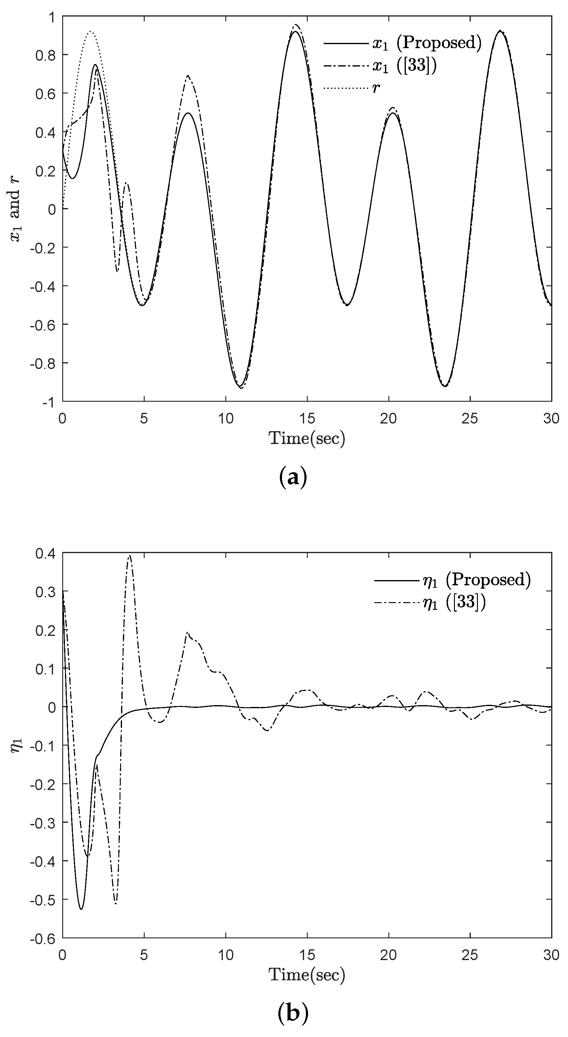
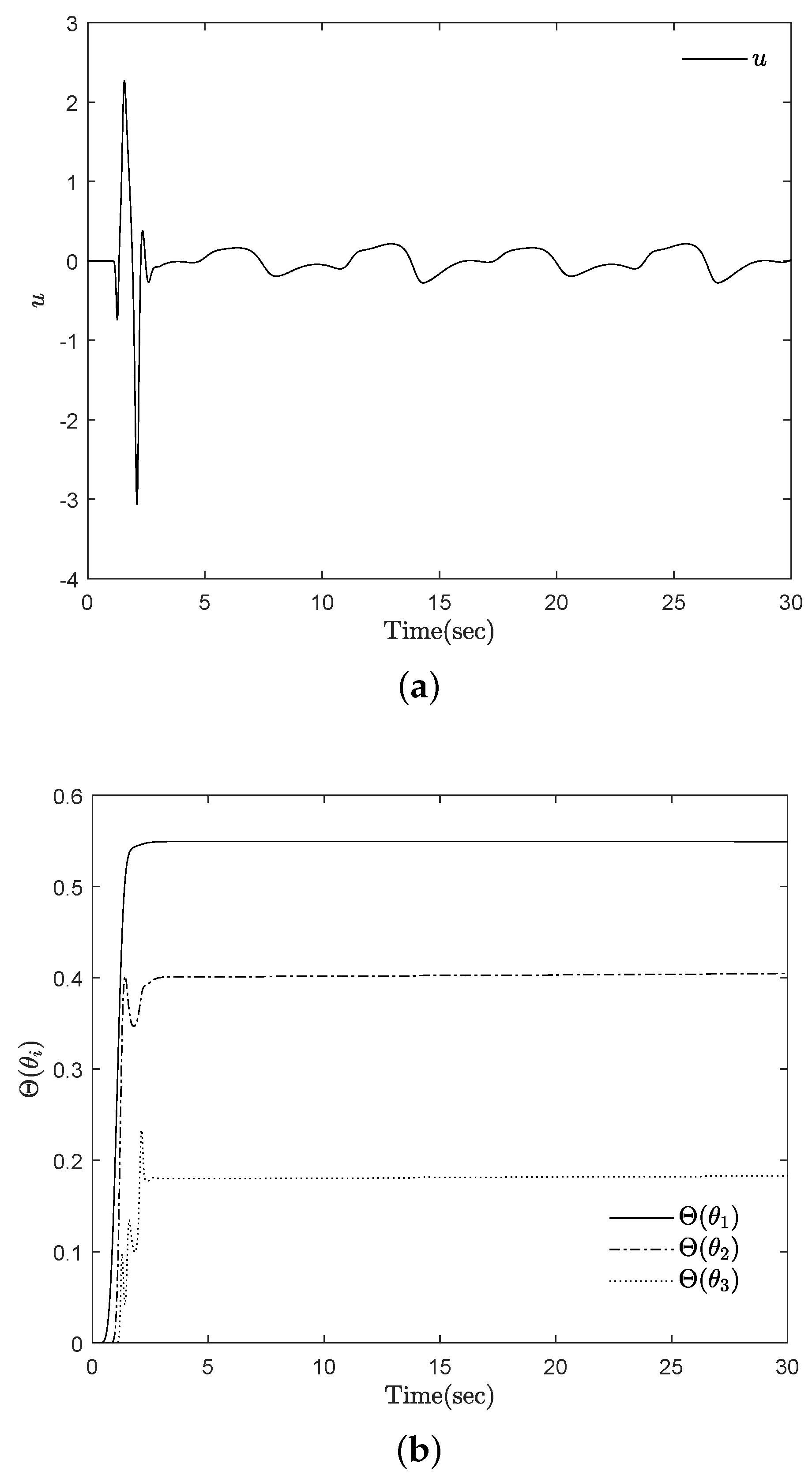
The tracking result and error are compared in Figure 2a,b, respectively. As shown in this figure, the tracking performance of the proposed controller is better than the previous controller using adaptive function approximators. Since the weights of the adaptive approximators should be updated on-line, the convergence speed of the tracking error of the controller [33] is slower than that of the proposed nonadaptive controller. Besides, the fluctuation of the tracking error in the transient response is mitigated by replacing the adaptive function approximator with the filter-based nonadaptive approximator. The IAE index values during 30 s are $0.8357$ for the proposed controller and $2.1412$ for the controller of [33]. Figure 3a,b depicts the control input and the outputs of the Nussbaum functions, respectively. The boundedness of u and $\Theta \left({\theta }_i\right)$, $i=1,2,3$, is shown. From these figures, we can conclude that the proposed approach presented in the filter-based control framework is effective for dealing with the problem of unknown control directions.

Example 2.

Chua’s circuit system has been widely investigated to describe prototypical electronic systems [45]. In this example, we consider the modified Chua circuit system [46] with an unknown sign of a control coefficient described by:

$$\begin{array}{c}{\dot{x}}_1={\varpi }_1(x_2-\frac{1}{7}(2x_1^3-x_1)),\hfill \\ {\dot{x}}_2=x_1-x_2+x_3,\hfill \\ {\dot{x}}_3=-{\varpi }_2{x}_2+u,\hfill \end{array}$$

(35)

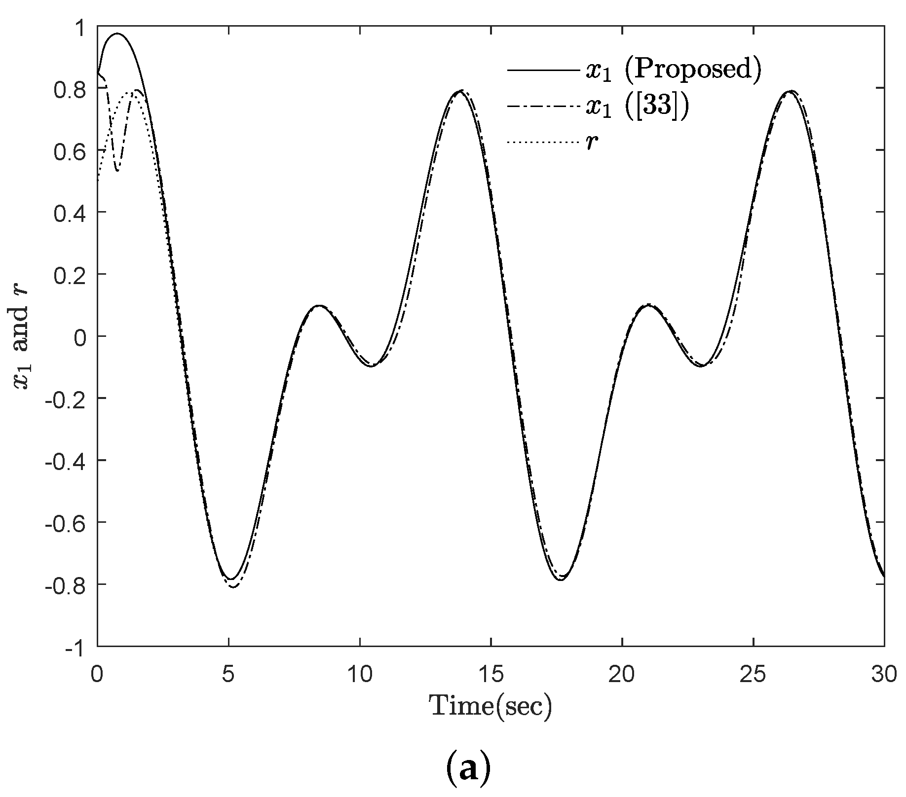
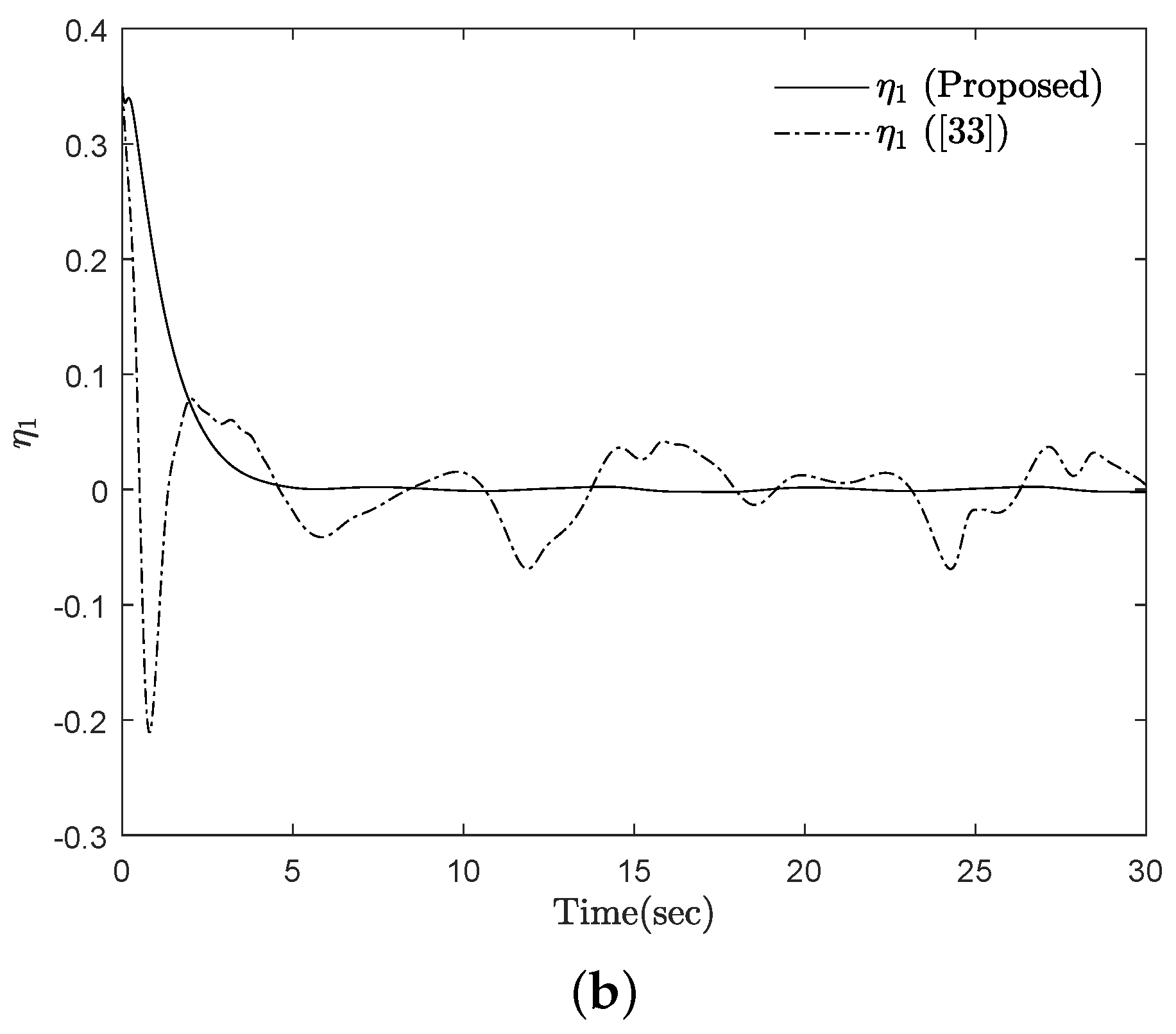
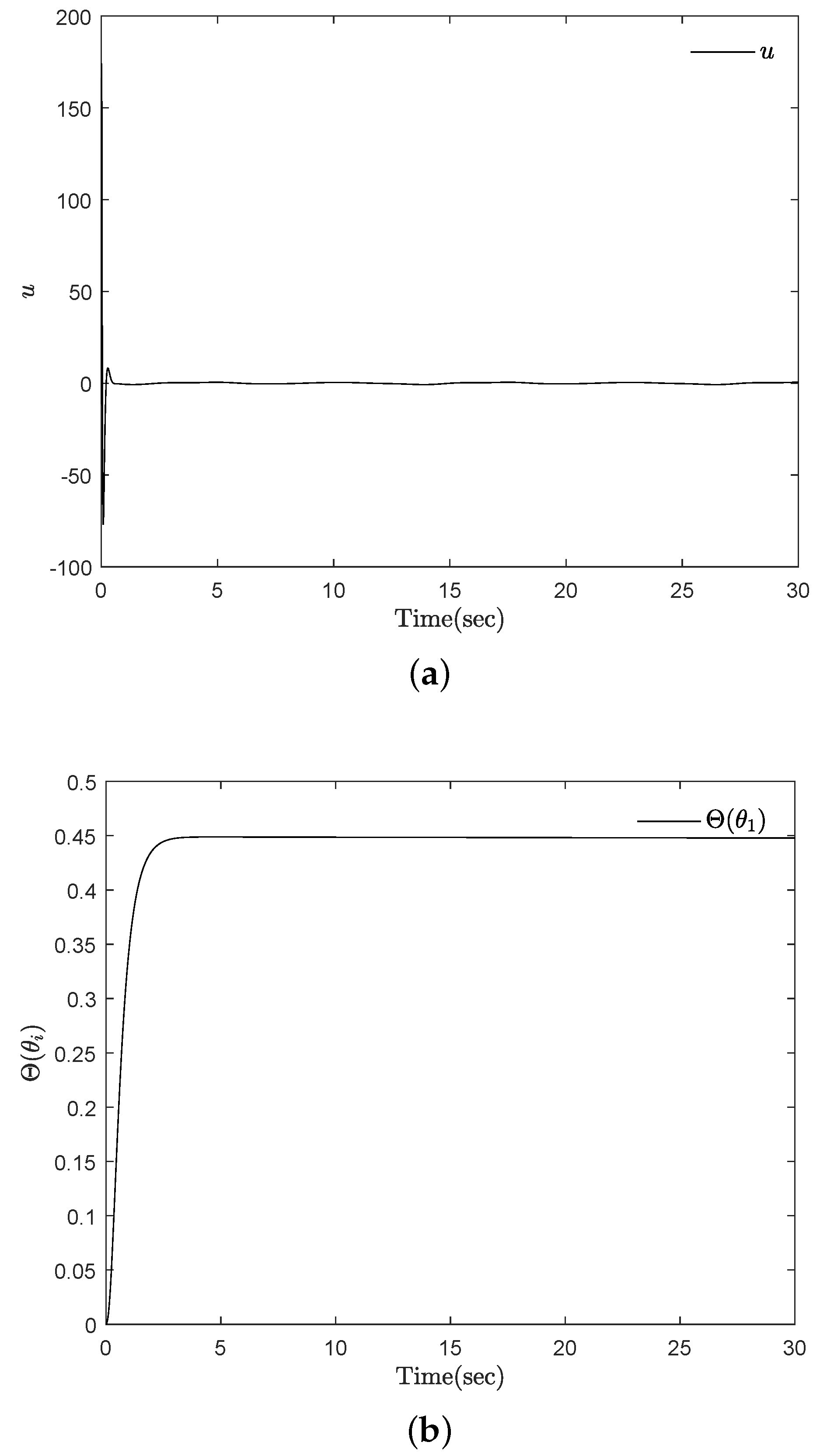
where ${\varpi }_1$ and ${\varpi }_2$ are unknown and nonzero system parameters, $x_1$ and $x_2$ are the voltages across two capacitors whose units are V, $x_3$ is the current through the inductor whose unit is A, and u is a voltage source added in series with the inductor whose unit is mV. We assume that the sign of the control coefficient ${\varpi }_1$ is unknown. For the simulation, we set ${\varpi }_1=1$, ${\varpi }_2=10/7$, ${\overline{x}}_3\left(0\right)={[-0.3,-0.5,0]}^{\top }$, ${\theta }_1\left(0\right)=0$, and $r\left(t\right)=0.5cos\left(0.5t\right)+0.7sin\left(t\right)$. The design parameters are selected as ${\tau }_i=0.025$, ${\gamma }_1=8.5$, ${\gamma }_2=3.5$, ${\gamma }_3=1$, and ${\delta }_2={\delta }_3=0.01$ where $i=1,2,3$. Figure 4 displays the tracking result and error of the proposed controller and the adaptive function approximation-based controller [33]. In Figure 4b, the IAE index values of the tracking error during 30 s are 0.5058 for the proposed controller and $0.9270$ for the controller [33]. From this figure, one can see that the tracking error under the proposed control scheme converges to the vicinity of zero in a few seconds, whereas the previous control scheme takes more time to converge. The control input and the output of the Nussbaum function are depicted in Figure 5a,b, respectively.

5. Conclusions

This paper presented a filter-based nonadaptive tracking design for the unknown control direction problem of uncertain pure-feedback nonlinear systems. Different from the existing adaptive recursive control designs, the major contribution of the proposed strategy is to achieve a simplified tracking control without using any adaptive approximators in the presence of unknown control directions. The control scheme using filtered signals of error surfaces, a control input, and state variables was constructed to achieve the semi-global practical tracking. The stability of the closed-loop system was thoroughly analyzed using the Lyapunov stability theorem, and simulation comparisons were provided to verify the effectiveness of the proposed control result. In our future study, we will analyze the control performance along with various Nussbaum-type functions and extend the filter-based approximation approach to the event-triggered control of network systems. Additionally, the potential application of the proposed controller includes vehicle vibration control in the stochastic wind field [47] and the traction power collector system subjected to unknown irregularities [48].

References

- Isidori, A. Nonlinear Control Systems: An Introduction; Springer: Berlin, Germany, 1989. [Google Scholar]
- Krstic, M.; Kanellakopoulos, I.; Kokotovic, P.V. Nonlinear and Adaptive Control Design; Wiley: New York, NY, USA, 1995. [Google Scholar]
- Swaroop, D.; Hedrick, J.K.; Yip, P.P.; Gerdes, J.C. Dynamic surface control for a class of nonlinear systems. IEEE Trans. Autom. Control 2000, 45, 1893–1899. [Google Scholar] [CrossRef] [Green Version]
- Liu, Y.J.; Tong, S. Barrier Lyapunov functions for Nussbaum gain adaptive control of full state constrained nonlinear systems. Automatica 2017, 76, 143–152. [Google Scholar] [CrossRef]
- Ge, S.S.; Hong, F.; Lee, T.H. Robust adaptive control of nonlinear systems with unkonwn time delays. Automatica 2005, 41, 1181–1190. [Google Scholar] [CrossRef]
- Yoo, S.J.; Park, J.B.; Choi, Y.H. Adaptive dynamic surface control for stabilization of parametric strict-feedback nonlinear systems with unknown time delays. IEEE Trans. Autom. Control 2007, 45, 2360–2365. [Google Scholar] [CrossRef]
- Zhou, J.; Wen, C.; Yang, G. Adaptive backstepping stabilization of nonlinear uncertain systems with quantized input signal. IEEE Trans. Autom. Control 2014, 59, 460–464. [Google Scholar] [CrossRef]
- Liu, Y.J.; Li, J.; Tong, S.; Chen, C.L.P. Neural network control-based adaptive learning design for nonlinear systems with full-state constraints. IEEE Trans. Neural Netw. Learn. Syst. 2016, 27, 1562–1571. [Google Scholar] [CrossRef] [PubMed]
- Yu, J.; Shi, P.; Dong, W.; Lin, C. Adaptive fuzzy control of nonlinear systems with unknown dead zones based on command filtering. IEEE Trans. Fuzzy Syst. 2018, 26, 46–55. [Google Scholar] [CrossRef]
- Li, D.P.; Liu, Y.J.; Tong, S.; Chen, C.L.P. Neural networks-based adaptive control for nonlinear state constrained systems with input delay. IEEE Trans. Cybern. 2019, 49, 1249–1258. [Google Scholar] [CrossRef]
- Li, D.P.; Liu, D.J. Adaptive neural tracking control for nonlinear time-delay systems with full state constraints. IEEE Trans. Syst. Man Cybern. Syst. 2017, 47, 1590–1601. [Google Scholar] [CrossRef]
- Zhou, Q.; Wu, C.; Jing, X.; Wang, L. Adaptive fuzzy backstepping dynamic surface control for nonlinear input-delay systems. Neurocomputing 2016, 199, 58–65. [Google Scholar] [CrossRef]
- Ge, S.S.; Hong, F.; Lee, T.H. Adaptive neural control of nonlinear time-delay systems with unknown virtual control coefficients. IEEE Trans. Syst. Man Cybern. Part Cybern. 2004, 34, 499–516. [Google Scholar] [CrossRef] [PubMed] [Green Version]
- Tong, S.; Li, Y. Fuzzy adaptive robust backstepping stabilization for SISO nonlinear systems with unknown virtual control direction. Inf. Sci. 2010, 180, 4619–4640. [Google Scholar] [CrossRef]
- Wen, Y.; Ren, X. Neural networks-based adaptive control for nonlinear time-varying delays systems with unknown control direction. IEEE Trans. Neural Netw. 2011, 22, 1599–1612. [Google Scholar] [PubMed]
- Yue, H.; Li, J. Output-feedback adaptive fuzzy control for a class of non-linear time-varying delay systems with unknown control directions. IET Control Theory Appl. 2012, 6, 1266–1280. [Google Scholar] [CrossRef]
- Yue, H.; Li, J. Output-feedback adaptive fuzzy control for a class of nonlinear systems with input delay and unknown control directions. J. Frankl. Inst. 2013, 350, 129–154. [Google Scholar] [CrossRef]
- Ma, J.; Zheng, Z.; Li, P. Adaptive dynamic surface control of a class of nonlinear systems with unknown direction control gains and input saturation. IEEE Trans. Cybern. 2015, 45, 728–741. [Google Scholar] [CrossRef]
- Yin, S.; Gao, H.; Qiu, J.; Kaynak, O. Adaptive fault-tolerant control for nonlinear system with unknown control directions based on fuzzy approximation. IEEE Trans. Syst. Man Cybern. Syst. 2017, 47, 1909–1918. [Google Scholar] [CrossRef]
- Askari, M.R.; Shahrokhi, M.; Talkhoncheh, M.K. Observer-based adaptive fuzzy controller for nonlinear systems with unknown control directions and input saturation. Fuzzy Sets Syst. 2017, 314, 24–45. [Google Scholar] [CrossRef]
- Tong, S.; Min, X.; Li, Y. Observer-based adaptive fuzzy tracking control for strict-feedback nonlinear systems with unknown control gain functions. IEEE Trans. Cybern. 2020. [Google Scholar] [CrossRef]
- Li, Y.; Tong, S.; Li, T. Composite adaptive fuzzy output feedback control design for uncertain nonlinear strict-feedback systems with input saturation. IEEE Trans. Cybern. 2015, 45, 2299–2308. [Google Scholar] [CrossRef]
- Yoo, S.J.; Park, J.B.; Choi, Y.H. Adaptive neural control for a class of strict-feedback nonlinear systems with state time delays. IEEE Trans. Neural Netw. 2009, 20, 1209–1215. [Google Scholar] [PubMed]
- Zhang, T.; Xia, M.; Yi, Y.; Shen, Q. Adaptive neural dynamic surface control of pure-feedback nonlinear systems with full state constraints and dynamic uncertainties. IEEE Trans. Syst. Man Cybern. Syst. 2017, 47, 2378–2387. [Google Scholar] [CrossRef]
- Li, Y.; Tong, S. Adaptive fuzzy output-feedback control of pure-feedback uncertain nonlinear systems with unknown dead zone. IEEE Trans. Fuzzy Syst. 2014, 22, 1341–1347. [Google Scholar] [CrossRef]
- Liu, Z.; Dong, X.; Xue, J.; Li, H.; Chen, Y. Adaptive neural control for a class of pure-feedback nonlinear systems via dynamic surface technique. IEEE Trans. Neural Netw. Learn. Syst. 2016, 27, 1969–1975. [Google Scholar] [CrossRef] [PubMed]
- Shen, Q.; Shi, P.; Zhang, T.; Lim, C.C. Novel neural control for a class of uncertain pure-feedback systems. IEEE Trans. Neural Netw. Learn. Syst. 2014, 25, 718–727. [Google Scholar] [CrossRef] [PubMed]
- Zhou, Q.; Wang, L.; Wu, C.; Li, H. Adaptive fuzzy tracking control for a class of pure-feedback nonlinear systems with time-varying delay and unknown dead zone. Fuzzy Sets Syst. 2017, 329, 36–60. [Google Scholar] [CrossRef]
- Wang, C.; Wu, Y.; Yu, J. Barrier Lyapunov functions-based dynamic surface control for pure-feedback systems with full state constraints. IET Control Theory Appl. 2017, 11, 524–530. [Google Scholar] [CrossRef]
- Yu, Z.; Li, S.; Yu, Z. Adaptive neural control for a class of pure-feedback nonlinear time-delay systems with asymmetric saturation actuators. Neurocomputing 2016, 173, 1461–1470. [Google Scholar] [CrossRef]
- Wang, H.; Sun, W.; Liu, P.X. Adaptive intelligent control of nonaffine nonlinear time-delay systems with dynamic uncertainties. IEEE Trans. Syst. Man Cybern. Syst. 2017, 47, 1474–1485. [Google Scholar] [CrossRef]
- Wang, H.; Chen, B.; Lin, C.; Sun, Y. Observer-based adaptive neural control for a class of nonlinear pure-feedback systems. Neurocomputing 2016, 171, 1517–1523. [Google Scholar] [CrossRef]
- Ren, B.; Ge, S.S.; Su, C.Y.; Lee, T.H. Adaptive neural control for a class of uncertain nonlinear systems in pure-feedback form with hysteresis input. IEEE Trans. Syst. Man Cybern. Part Cybern. 2009, 39, 431–443. [Google Scholar]
- Zhang, T.; Shi, X.; Zhu, Q.; Yang, Y. Adaptive neural tracking control of pure-feedback nonlinear systems with unknown gain signs and unmodeled dynamics. Neurocomputing 2013, 121, 290–297. [Google Scholar] [CrossRef]
- Chen, Q.; Shi, L.; Na, J.; Ren, X.; Nan, Y. Adaptive echo state network control for a class of pure-feedback systems with input and output constraints. Neurocomputing 2018, 275, 1370–1382. [Google Scholar] [CrossRef]
- Lai, X.; Pan, H.; Zhao, X. Adaptive control for pure-feedback nonlinear systems preceded by asymmetric hysteresis. Energies 2019, 12, 4675. [Google Scholar] [CrossRef] [Green Version]
- Na, J.; Yang, J.; Wang, S.; Gao, G.; Yang, C. Unknown dynamics estimator-based output-feedback control for nonlinear pure-feedback systems. IEEE Trans. Syst. Man Cybern. Syst. 2019. [Google Scholar] [CrossRef]
- Zhang, L.; Yang, G.-H. Fault-estimation-based output-feedback adaptive FTC for uncertain nonlinear systems With actuator faults. IEEE Trans. Ind. Electron. 2020, 67, 3065–3075. [Google Scholar] [CrossRef]
- Bu, X. Guaranteeing prescribed performance for air-breathing hypersonic vehicles via an adaptive non-affine tracking controller. Acta Astronaut. 2018, 151, 368–379. [Google Scholar] [CrossRef]
- Kanellakopoulos, I.; Kokotovic, P.V.; Morse, A.S. Systematic design of adaptive controllers for feedback linearizable systems. IEEE Trans. Autom. Control 1991, 36, 1241–1253. [Google Scholar] [CrossRef] [Green Version]
- Choi, Y.H.; Yoo, S.J. Filter-driven-approximation-based control for a class of pure-feedback systems with unknown nonlinearities by state and output feedback. IEEE Trans. Syst. Man Cybern. Syst. 2018, 48, 161–176. [Google Scholar] [CrossRef]
- Wang, C.; Hill, D.J.; Ge, S.S.; Ghen, G. An ISS-modular approach for adaptive neural control of pure-feedback systems. Automatica 2006, 42, 723–731. [Google Scholar] [CrossRef]
- Nussbaum, R.D. Some remarks on a conjecture in parameter adaptive control. Syst. Control Lett. 1983, 3, 243–246. [Google Scholar] [CrossRef]
- Apostol, T.M. Mathematical Analysis; Addison-Wesley: Reading, UK, 1974. [Google Scholar]
- Madan, R.N. Chua’s Circuit: A Paradign for Chaos; World Scientific: Singapore, 1993. [Google Scholar]
- Hwang, C.C.; Chow, H.Y.; Wang, Y.K. A new feedback control of a modified Chua’s circuit system. Phys. D 1996, 92, 95–100. [Google Scholar] [CrossRef]
- Baker, C.; Cheli, F.; Orellano, A.; Paradot, N.; Proppe, C.; Rocchi, D. Cross-wind effects on road and rail vehicles. Veh. Syst. Dyn. 2009, 47, 983–1022. [Google Scholar] [CrossRef]
- Song, Y.; Liu, Z.; Rønnquist, A.; Nåvik, P.; Liu, Z. Contact Wire Irregularity Stochastics and Effect on High-speed Railway Pantograph-Catenary Interactions. IEEE Trans. Instrum. Meas. 2020. [Google Scholar] [CrossRef]
Figure 1.
Block diagram of the proposed filter-based nonadaptive tracking system.
Figure 2.
Comparison of the tracking result and error for Example 1: (a) and r; (b) .
Figure 3.
The control input and the Nussbaum functions’ outputs for Example 1: (a) u; (b) , .
Figure 4.
Tracking result and error for Example 2: (a) and (b) .
Figure 5.
The control input and the Nussbaum function’s output for Example 2: (a) u; (b) .
© 2020 by the authors. Licensee MDPI, Basel, Switzerland. This article is an open access article distributed under the terms and conditions of the Creative Commons Attribution (CC BY) license (http://creativecommons.org/licenses/by/4.0/).
Share and Cite
MDPI and ACS Style
Choi, Y.H.; Yoo, S.J. Tracking Control Strategy Using Filter-Based Approximation for the Unknown Control Direction Problem of Uncertain Pure-Feedback Nonlinear Systems. Mathematics 2020, 8, 1341. https://doi.org/10.3390/math8081341
AMA Style
Choi YH, Yoo SJ. Tracking Control Strategy Using Filter-Based Approximation for the Unknown Control Direction Problem of Uncertain Pure-Feedback Nonlinear Systems. Mathematics. 2020; 8(8):1341. https://doi.org/10.3390/math8081341
Chicago/Turabian StyleChoi, Yun Ho, and Sung Jin Yoo. 2020. "Tracking Control Strategy Using Filter-Based Approximation for the Unknown Control Direction Problem of Uncertain Pure-Feedback Nonlinear Systems" Mathematics 8, no. 8: 1341. https://doi.org/10.3390/math8081341
Note that from the first issue of 2016, this journal uses article numbers instead of page numbers. See further details here.