


Abstract
Far-field directional scattering and near-field directional coupling from simple sources have recently received great attention in photonics: beyond circularly-polarized dipoles, whose directional coupling to evanescent waves was recently applied to acoustics, the near-field directionality of modes in optics includes phased combinations of electric and magnetic dipoles, such as the Janus dipole and the Huygens dipole, both of which have been experimentally implemented using high refractive index nanoparticles. In this work we extend this to acoustics: we propose the use of high acoustic index scatterers exhibiting phased combinations of acoustic monopoles and dipoles with far-field and near-field directionality. All solutions stem from the elegant angular spectrum of the acoustic source, in close analogy to electromagnetism. A Huygens acoustic source with zero backward scattering is proposed and numerically demonstrated, as well as a Janus source achieving face-selective and position-dependent evanescent coupling to nearby acoustic waveguides.
Export citation and abstract BibTeX RIS

Original content from this work may be used under the terms of the Creative Commons Attribution 4.0 licence. Any further distribution of this work must maintain attribution to the author(s) and the title of the work, journal citation and DOI.
1. Introduction
In electromagnetism and photonics, high index dielectric particles are becoming an important platform to study novel physical phenomena [1]. Unlike plasmonic nanoparticles, a high index dielectric particle can exhibit strong magnetic Mie resonances [2, 3] that are of comparable strength to the electric ones. Sources such as the Huygens and Janus dipoles show interesting directional scattering and coupling characteristics, both in the far field and in the near field [4, 5], and they have been experimentally demonstrated in high-index nanoparticles [6–9] with interfering electric p and magnetic m dipole moments. In the far-field, the combination of orthogonal p and m dipoles following Kerker's condition p = m/c gives rise to the Huygens dipole, exhibiting directional scattering [6–8] with applications in reflectionless metasurfaces [1, 10, 11] and optical metrology [12] among others. In the near-field, directional coupling of waveguided modes was initially predicted and demonstrated in electromagnetism via the evanescent coupling of circularly polarised dipoles [13], relying on the transverse spin and spin-momentum locking in evanescent waves [14–16]. The acoustic analogy of electromagnetic dipoles was recently introduced in reference [17], which also theoretically reavealed the presence of transverse spin angular momentum in an acoustic evanescent wave. The acoustic spin-momentum locking was experimentally demonstrated using circular acoustic dipoles [18, 19]. This shows that the transverse spin is a universal property of evanescent waves in any wave field including acoustics [17–21], electromagnetism [14–16] and gravitational waves [22]. However, near-field directionality in electromagnetism was generalised beyond circular dipoles to include combinations of electric and magnetic dipoles that achieve near-field directional coupling with different symmetries [4, 5]: one example is the aforementioned Huygens dipole, which can be also applied for near-field directionality, and another is the intriguing Janus dipole, whose combination between electric and magnetic dipoles requires a 90° phase difference to achieve a face-dependent or position-dependent coupling to the waveguide modes [4]. These sources exploit the amplitude and phase relations that exist between different components of the electric and magnetic fields in evanescent waves. In acoustics, similar amplitude and phase relations exist between the scalar pressure and vector velocity fields, opening the possibility of Huygens and Janus-like directional sources.
High index materials are also sought after in acoustics [23, 24]. Micro-sized air bubbles in liquid show strong resonances [25] and are widely used as a contrast agent for high resolution acoustic imaging [26]. Acoustic metamaterials [27, 28] made of high index materials are proposed to achieve exotic physical properties like negative effective mass density and modulus [29, 30]. High index materials are also important in bringing functionalities such as waveguiding from advanced electromagnetism and photonics into acoustics [24]. Mie-type acoustic meta-atoms [31–33] have been proposed and demonstrated, which can have high effective acoustic index even in an air background. In this work we explore the possibility to produce acoustic Huygens and Janus-type directional sources to achieve far and near-field directionality, using a high-index particle platform.
2. Theory
We begin this work by deriving all possible combinations of an acoustic monopole M and dipole D that achieve far- and near-field directionality. The complex pressure field of such a source is given by:

where r = |r| is the distance to the source, assumed to be at the origin, and k0 = 2π/λ is the acoustic wave-number of free space. To analyse both far- and near-field directionality we will apply a standard technique in electromagnetism: the angular spectrum decomposition [34–37]. Such decomposition expands the fields as a superposition of momentum eigenmodes p(r) = ∫kp(k)eik⋅rdk. Each component p(k)eik⋅r has a constant wave-vector k = (kx, ky, kz). Owing to the dispersion relation, the kz component of k can be derived from the in-plane momentum (kx, ky) via the dispersion relation  . As is well-known in photonics, in the region
  the momentum eigenmodes correspond to propagating plane waves with a real-valued k. However, in the region
  , the component kz becomes imaginary, and eik⋅r represents an evanescent wave, corresponding to the near-field spectrum [38].
The angular spectrum p(k) can be analytically calculated via a partial Fourier transform of p(r) from equation (1), using Weyl's identity [36], and it is given as (see appendix

where  . Equation (2) is the master equation from which any type of directionality can be analysed or designed. Far-field directionality manifests itself as zeroes in the angular spectrum inside the circle
  , while near-field directionality manifests itself as zeroes outside of that circle [4, 5, 39]. For example, let us start with far-field directionality: to achieve directionality in the forward x direction we may introduce a zero of p(k) for the plane wave propagating along the negative x axis. Substituting
  into equation (2) and equating it to zero, one immediately arrives at the acoustic analogue of Kerker's condition M − Dx = 0. An acoustic monopole M combined with an acoustic dipole D = (M, 0, 0) will result in Kerker-like far-field directionality, in complete analogy to a Huygens' dipole. This is shown in the far-field diagrams of figure 1. Intuitively, the monopole source is expanding and contracting in an oscillating manner, creating an isotropic spherical pressure wave, while the dipolar source is vibrating back and forth, creating a peanut-like radiation diagram, with opposite pressure changes and opposite velocities on opposite directions. Their coherent combination results in a very special vibration of the source: the source moves forwards while expanding, and then moves backwards while contracting, in such a way that the backward-facing surface does not move, producing no pressure wave in the backward direction. In the next section we show how to implement this acoustic Huygens source in a realistic spherical or cylindrical scatterer upon plane wave excitation, exhibiting no back-scattering, with interesting applications.

Figure 1. Analogy between far field directionality (Kerker's condition) in electromagnetic and acoustic scattering.
Download figure:
Standard image High-resolution imageEven more interesting solutions appear if we look at near-field directionality. In this case, we must set the angular spectrum in equation (2) to be zero at some value of (kx, ky) outside of the circle  . Following an identical approach to the optical case [5, 35, 39], we can study near-field directional coupling to a waveguided mode with an effective refractive index neff. The evanescent wave near-field component that would couple to such a mode, propagating in the ±x direction, is given by
  , where
  to fulfil the wave-equation condition
  . The sign of ±neff will determine the direction of propagation of the mode, +x or −x, while the sign of γ will determine the position of the source, below or above the waveguide, respectively. Substituting this
  into equation (2), and equating it to zero, we immediately arrive at M + neffDx + iγDz = 0. Three simple solutions emerge when only two of the three source components are allowed to be non-zero: (i) the circularly polarized dipole, (ii) the near-field Huygens dipole, and (iii) the Janus dipole. The three solutions are summarized in table 1 and simulated numerically in Comsol by placing the different sources near a waveguide, shown in figure 2. The sources are a clear mathematical analogy to their electromagnetic counterparts [4]. While in electromagnetism we could find two versions of each solution—corresponding to each of the two transverse polarizations—in acoustics there is only one version of each solution, consistent with the fact that acoustic waves have a single longitudinal polarisation. In the next section we show how high acoustic index particles can be used to achieve these solutions, with the required relative amplitudes and phases between the monopole and dipole components, and numerically demonstrate Huygens and Janus behaviour in the far-field and near-field, respectively.
Table 1. Elemental monopole and dipole combinations for near-field directionality in planar waveguides.
| Source | Condition |
|---|---|
| Circular |  |
| Huygens | M = −neffDx |
| Janus |  |
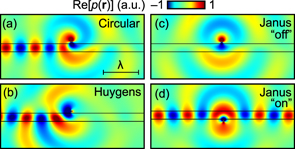
Figure 2. Near-field directional coupling using acoustic monopole and dipole combinations. (a) Circular dipole, (b) Huygens source, (c) and (d) Janus source. The waveguide slab has  , thickness 0.2λ, and neff ≈ 1.31. The source is placed at a distance 0.05λ above (a)–(c) or below (d) the waveguide.
Download figure:
Standard image High-resolution image3. High index acoustic scatterers
Consider a high index acoustic scatterer upon which an external, time-harmonic sound wave with pressure distribution pin(r) and velocity field  is incident. We assume the scatterer is located at r = 0 in a background with mass density ρ0 and compressibility β0 and only longitudinal sound waves with velocity
  considered. The monopole and dipole induced in the acoustic scatterer are given by:

where pin and vin are evaluated at r = 0, and αM and αD represent the acoustic monopolar and dipolar strength, solely determined by the scatterer and the background material. In the special case of plane wave or evanescent wave incidence  , the dipole moment is reduced to
  and the master equation for the angular spectrum of the scattered field, equation (2), can be simplified as:

In order to illustrate our concept in a simple manner but without loss of generality, let us assume the scatterer is a sphere of radius r0 and made of a material that supports longitudinal sound waves only, and has a relative mass density and compressibility  and
and  . The acoustic scattering of spheres and cylinders can be analytically calculated (as detailed in appendices
  corresponds to a strong contrast in the speed of sound between the scatterer and the background medium c1 = c0/n. Just like the electromagnetic case, where a high refractive index results in a spectral region (i.e. certain values of 2πr0/λ) dominated by the electric and magnetic dipolar contribution, a high index in acoustics also results in a spectral region of strong acoustic monopolar and dipolar responses, with the higher order modes suppressed.
The relative amplitude and phase between the monopolar and dipolar strength can be tuned with the material properties and size, enabling us to easily achieve the specific conditions required for Huygens and Janus sources. Figure 3 shows the relative amplitude and phase of the acoustic monopolar and dipolar moments for a sphere with an acoustic index n = 3, with varying relative mass density  and compressibility
  . In the range shown, 0 < 2πr0/λ < 1.5, the higher order multipoles are negligible. We begin by looking at the conditions required for a Huygens-type far-field directional particle. Following equation (4), the scattering pressure of the particle in the forward/backward direction, relative to the incident plane wave, is given by
 ![$p\left({\pm}{\hat{\mathbf{k}}}_{\text{in}}{k}_{0}\right)\propto {\alpha }_{\mathrm{M}}+{\alpha }_{\mathrm{D}}\left[\left({\pm}{\hat{\mathbf{k}}}_{\text{in}}\right)\cdot {\hat{\mathbf{k}}}_{\text{in}}\right]$](https://content.cld.iop.org/journals/1367-2630/22/8/083016/revision3/njpab9fbfieqn24.gif) . Owing to the dispersion relation, we know that
. Owing to the dispersion relation, we know that  , and so, the condition to achieve zero forward/backward scattering becomes:


Figure 3. Relative amplitude (a) and phase (b) of the acoustic monopolar and dipolar moment strengths αM and αD for a sphere with acoustic index n = 3. The black dashed lines indicate the parametric locations where |αM/αD| = 1, and the white dashed lines indicate the parametric locations where arg{αM/αD} = π/2.  and
and  are the relative mass density and compressibility of the scatterer compared to the background medium.
Download figure:
Standard image High-resolution imageThe condition for no backward scattering is therefore αM = αD, and it can be easily implemented with a subwavelength particle. Consider the behaviour shown in figure 3(b) in the limit of small particles (r0/λ → 0). In this limit, we can see three distinct regions: the monopolar and dipolar moments are ±π out of phase (preferred backward scattering) in the ranges  and
and  , while they are in phase (preferred forward scattering) in the overlapping region where both
  and
and  are larger than 1. This result can be derived analytically: in the limit r0/λ → 0, the two moments can be approximated as
  and
and  . In the region where both monopole and dipole are in phase, there is a point where they also have equal amplitudes, marked with a black dashed line, and so αM = αD. This condition represents the acoustic analog of the electromagnetic Huygens dipole with zero back-scattering in the far field, easily achievable with high-index spheres or cylinders. A numerical simulation using the acoustic module of COMSOL multiphysics (see details of the simulation in appendix

Figure 4. (a) Scattered pressure distribution of a cylinder (radius r0 = 0.2λ/(2π), relative acoustic index n = 3 and relative mass density  ) upon plane wave incidence along the +
 direction, where the Huygens condition αM = αD for zero backward scattering is met. (b) and (c) Scattered pressure distribution of a cylinder (radius r0 = 0.287λ/(2π), relative acoustic index n = 8.082 and relative mass density
  ) placed at a distance of λ/8 below (in (b)) or above (in (c)) a slab waveguide (thickness λ/6, relative acoustic index n = 1.81 and relative mass density
  ). A sound plane wave is incident along the +
 direction. The cylinder scatterer fulfils the Janus condition with αM/αD = 0.599i and the slab waveguide supports a guided mode with effective index neff ≈ 1.166.
Download figure:
Standard image High-resolution image
The Janus condition can also be achieved, but not in the limit of small particles. The white dashed lines in figure 3 indicate the locations where the monopole and dipole moments are on quadrature phase difference αM/αD = i|αM/αD| as required by Janus sources. The specific required amplitude ratio |αM/αD| will depend on the effective index of the modes we want to couple to. Assume that the incident sound wave is propagating in the  direction, i.e.
  . Following equation (4), the scattering angular spectrum for evanescent wavevectors kev with
  , and corresponding kz = ±ik0γ, is given by:

where we introduced the Janus condition αM/αD = i|αM/αD|, and where  is always taken as the positive square root, while the ± sign corresponds to scattering in the z > 0 or z < 0 half spaces, respectively. It follows from equation (6) that the evanescent components with a transverse wavevector satisfying
  , will have a zero amplitude in the lower half space (z < 0), meaning that the source will not couple to waveguided modes with an effective index neff when the waveguide is placed in the z < 0 half-space. At the same time, the source has a non-zero amplitude for the same evanescent waves in the upper half space (z > 0), meaning that it will couple to the modes of the same waveguide if it is placed in the z > 0 half-space. This, together with no far-field directionality—which is easy to prove for these monopole and dipole compositions αM/αD = i|αM/αD|—constitutes the signature of a Janus source, with its charcteristic face-dependent behaviour, in perfect analogy to electromagnetism. Figures 4(b) and (c) shows a cylindrical particle designed in this way, simulated in COMSOL (details of the simulation are given in appendix
Our calculations and simulations above have neglected the presence of losses in order to present a clearer picture and describe the novel physics. In practice, the presence of losses is unavoidable and should be taken into account as an experimental reality. Fortunately, the presence of losses perturbs our results in a smooth way, with no sudden change in behaviour: low losses result in negligible effects, and increasing them broadens the resonances, changing the phase difference and amplitude ratios between the monopolar and dipolar responses in a continuous way, as expected, but without altering the physical arguments given above.
4. Conclusion and discussions
We have extended the analogy of far and near-field directionality from dipolar sources in electromagnetism to the domain of acoustics. On one hand, we theoretically describe and numerically demonstrate the acoustic analogy of a far-field directional Huygens dipole with zero back-scattering, implemented with high acoustic index spheres or cylinders. These resonant scatterers, like their electromagnetic/photonic counterparts, can function as subwavelength acoustic antennas, offering some new freedom in constructing acoustic metasurfaces to generate structured acoustic waves. This may have interesting application for reduced reflection materials in acoustics engineering. The possibility of zero forward-scattering Huygens scatterers could also lead to the design of novel sound barriers. On the other hand, we also theoretically described near-field directional coupling of waveguided modes using monopole and dipole combinations. We show that the three solutions: circular dipole, Huygens source, and Janus source, in perfect analogy to the electromagnetic case, appear naturally as independent solutions to the simple angular spectrum of an acoustic source. We theoretically and numerically propose a simple realistic way of achieving a Janus scatterer with spherical or cylindrical high acoustic index materials, clearly exhibiting the characteristic position-dependent near-field coupling behaviour. This has clear implications for the understanding and control of the near-fields of sound waves.
Extending the concept of near-field directionality of electromagnetic Janus, Huygens and circular dipoles to acoustics has clear implications for the understanding and control of the near-fields of sound waves. These sources can be used to directionally couple sound waves to acoustic waveguides or metasurfaces. The characteristic symmetry of the three types of acoustic source can be further explored to study their interactions with topological acoustic structures. Our results present new applications of low loss high acoustic index scatters, which should motivate practical designs. Furthermore, the separate control of acoustic monopole and dipole by pressure and velocity fields of the incident sound wave can be used to explore the interactions, including acoustic forces, between a structured sound wave (evanescent waves or bessel beam or vortex beam) and a designed acoustic scatterer.
During the writing of this manuscript we noticed the recent publication of reference [40] which describes a similar concept of acoustic near-field directional sources as described here. While reference [40] proposes sources realization using phased arrays of acoustic monopoles, our work devises the sources based on an angular spectrum approach and proposes the realization of both far-field and near-field directional sources using high index acoustic scatterers.
Acknowledgments
This work is supported by European Research Council Starting Grant No. ERC-2016-STG-714151-PSINFONI.
Appendix A.: Scattering coefficients of spherical particle and angular spectrum of acoustic monopole and dipole
In this work, we consider an acoustic scatterer with dominant monopolar and dipolar responses, subject to an external time-harmonic sound wave with a pressure distribution  and
and  . We assume that the scatterer is located at the origin r = 0 in a fluidic background with mass density ρ0 and compressibility β0 and only longitudinal sound waves being considered. The longitudinal sound velocity of the background medium is
  with k0 = 2π/λ being the wave-number of the background medium and λ the wavelength of the sound wave.
The contribution of the monopolar and dipolar responses of the acoustic scatterer to the total scattering is purely determined by the monopole moment M and dipole moment D:

where  is the velocity field of the incident sound wave, αM = a0/i and αD = 3a1/i represent the monopole and dipole strength of the scatterer, and where a0 and a1 are coefficients for the monopole and dipole, solely determined by the scatterer itself. For the special case of a spherical object, its scattering of sound waves can be analytically treated like Mie theory for optical scattering. Consider a spherical scatterer with a radius of r0 and made of materials with mass density ρ1 and compressibility β1, supporting longitudinal sound waves with a velocity
  . The coefficients a0 and a1 can be determined by the following expression:

where jn(kr) is the spherical Bessel function of the first kind and  is the spherical Hankel function of the first kind, j'n(kr) and
  are their first order derivatives with respect to the argument variable kr. The relative mass density and compressibility are defined as
  and
and  , and k1 = ω/c1 = k0n with
  being the acoustic refractive index.
The scattering pressure distribution due to the monopole and dipole contribution can be expressed as:

In order to obtain the angular spectrum of this source, we need to perform a partial Fourier transform in the xy plane. The angular spectrum p(kx, ky) is defined such that:

where the z direction is an arbitrarily defined direction in space, so that kz is taken to be the dependent variable  while the angular spectrum is defined in the two dimensional domain of transverse wave-vectors p(k) = p(kx, ky). As is well-known in electromagnetism, strictly speaking two different spectra p+(kx, ky) and p−(kx, ky) have to be defined, corresponding to the fields in the z > 0 halfspace and the z < 0 halfspace, corresponding to the two possible signs of kz, respectively.
In order to write equation (A3) in the form of equation (A4), we make use of Weyl's identity [36]:

Substituting Weyl's identity into the corresponding terms in equation (A3), and applying the linearity of the integration and gradient operations (the gradient operator becomes a multiplication times ik inside the integral) we arrive at:

where  . By comparing equation (A6) with the definition of the angular spectrum in equation (A4), we finally identify the expression for the angular spectrum:

as given in the main text. Note that the two angular spectra p+(kx, ky) and p−(kx, ky), corresponding to the two half spaces z > 0 and z < 0 will differ in the sign of the z component of the vector  . Also note that equation (A7) is a complete and exact analytical form of the angular spectrum, revealing not only the far-field directionality of the source (for
  ) but also its near-field directionality (corresponding to the evanescent wave spectrum when
  ) associated to the coupling behaviour between this source and nearby bound waveguide modes.
Appendix B.: Scattering coefficients of cylindrical particles
The scattering of a cylindrical particle can also be treated analytically. Assume the cylinder is of infinite length along y and the sound wave is incident in the xz plane. The scattering problem is then reduced to a 2D case. The monopole and dipole strength of a cylindrical scatterer can be determined as αM = a0/i and αD = 2a1/i, with the acoustic Mie coefficients a0 and a1 determined by the following expression:

where Jn(kr) is the Bessel function of the first kind and  is the Hankel function of the first kind, J'n(kr) and
  are their first order derivatives with respect to the argument variable kr.
The scattering pressure distribution due to the monopole and dipole contribution in the 2D case can be expressed as:

where  is the zero order Hankel function of the first kind and
  .
.
Since the cylinder is infinite along y and the incoming sound wave is incident in the xz plane, the partial Fourier transform of the pressure field can be performed along the x-axis only:

where the z direction is an arbitrarily defined direction in space, so that kz is taken to be the dependent variable  while the angular spectrum is defined by the transverse wave-vector p(k) = p(kx) and ky = 0. As is well-known in electromagnetism, strictly speaking two different spectra p+(kx) and p−(kx) have to be defined, corresponding to the fields in the z > 0 halfspace and the z < 0 halfspace, corresponding to the two possible signs of kz, respectively.
Following reference [41], the angular spectrum representation of  can be derived as

Substituting equation (B4) into the corresponding terms in equation (B2), we arrive at the angular spectrum representation of the cylinder's scattering pressure field in the monopole and dipole approximation:

By comparing equations (B5) and (B3), we can identify the angular spectrum of the cylinder's scattering pressure field

From equations (B6) and (A7), the scattering field angular spectrum of both the 3D sphere and the 2D cylinder are determined by the same master relation ![$\left[M+\left(\hat{\mathbf{k}}\cdot \mathbf{D}\right)\right]$](https://content.cld.iop.org/journals/1367-2630/22/8/083016/revision3/njpab9fbfieqn63.gif) in the acoustic monopole and dipole approximation.
in the acoustic monopole and dipole approximation.
Appendix C.: Numerical simulations
The numerical simulations in this work including the results shown in figures 2 and 4 are performed using the acoustic module of COMSOL multiphysics. The wave equations for time-harmonic monochromatic sound waves of angular frequency ω are solved:

where p and v are the pressure and velocity fields, and the material properties including mass density ρ and compressibility β are considered to be lossless.
In actual simulations, we first determine the geometrical and material parameters of the cylindrical scatterer analytically so that the acoustic Mie coefficients in equation (B1) meet the requirement of a Huygens source (as in figure 4(a)) and a Janus source (as in figures 4(b) and (c)).
In figure 4(a), the scattered pressure distribution of an isolated cylinder of radius r0 = 0.2λ/(2π) with relative acoustic index n = 3 and relative mass density  is numerically simulated using COMSOL, upon plane wave incidence along the +
 direction. A perfect matching layer is added outside the calculation region to address the open boundaries.
In figures 4(b) and (c), the scattered pressure distributions of a cylinder [radius r0 = 0.287λ/(2π), relative acoustic index n = 8.082 and relative mass density  ] placed at a distance of λ/8 below (in (b)) and above (in (c)) a slab waveguide (thickness λ/6, relative acoustic index n = 1.81 and relative mass density
  ) are calculated. A sound plane wave is incident along the + direction. The parameters of the cylindrical scatterer are determined analytically to induce a Janus source that matches the corresponding effective index of the guide mode of the adjacent slab waveguide. The total pressure fields with scatterer and slab waveguide as well as the case with only slab waveguide are numerically calculated using COMSOL. The scattered fields shown in figures 4(b) and (c) are obtained by subtracting the two. In the numerical simulations, we use a finite slab waveguide with a length of around 30.5λ to reduce the reflection at the edge. A perfect matching layer is added outside the calculation region. The finite slab waveguide does not affect the physics here.