Article

A Robust Electric Spring Model and Modified Backward Forward Solution Method for Microgrids with Distributed Generation

by
Guillermo Tapia-Tinoco
1,
David Granados-Lieberman
2,
David A. Rodriguez-Alejandro
2,
Martin Valtierra-Rodriguez
3 and
Arturo Garcia-Perez
1,*
1
Engineering Division, University of Guanajuato, Campus Irapuato-Salamanca, Carretera Salamanca-Valle de Santiago km 3.5 + 1.8 km, comunidad de Palo Blanco, C.P. 36885 Salamanca, Gto., Mexico
2
ENAP-Research Group, Department of Electromechanical Engineering, National Technological Institute of Mexico, Instituto Tecnológico Superior de Irapuato (ITESI), Carr. Irapuato-Silao km 12.5, Colonia el Copal, C.P. 36821 Irapuato, Gto., Mexico
3
ENAP-Research Group, Faculty of Engineering, Autonomous University of Queretaro, Campus San Juan del Río, Río Moctezuma 249, col. San Cayetano, C.P. 76807 San Juan del Río, Qro., Mexico
*
Author to whom correspondence should be addressed.
Mathematics 2020, 8(8), 1326; https://doi.org/10.3390/math8081326
Submission received: 1 July 2020 / Revised: 31 July 2020 / Accepted: 5 August 2020 / Published: 10 August 2020
(This article belongs to the Special Issue Mathematical Methods applied in Power Systems)

Abstract

:
The electric spring (ES) is a contemporary device that has emerged as a viable alternative for solving problems associated with voltage and power stability in distributed generation-based smart grids (SG). In order to study the integration of ESs into the electrical network, the steady-state simulation models have been developed as an essential tool. Typically, these models require an equivalent electrical circuit of the in-test networks, which implies adding restrictions for its implementation in simulation software. These restrictions generate simplified models, limiting their application to specific scenarios, which, in some cases, do not fully apply to the needs of modern power systems. Therefore, a robust steady-state model for the ES is proposed in this work to adequately represent the power exchange of multiples ESs in radial micro-grids (µGs) and renewable energy sources regardless of their physical location and without the need of additional restrictions. For solving and controlling the model simulation, a modified backward–forward sweep method (MBFSM) is implemented. In contrast, the voltage control determines the operating conditions of the ESs from the steady-state solution and the reference voltages established for each ES. The model and algorithms of the solution and the control are validated with dynamic simulations. For the quasi-stationary case with distributed renewable generation, the results show an improvement higher than 95% when the ESs are installed. On the other hand, the MBFSM reduces the number of iterations by 34% on average compared to the BFSM.

1. Introduction

The integration of renewable energy sources, the technological evolution of electric vehicles, and the development of more efficient and higher capacity energy storage systems are some alternatives to restrain CO2 gas emissions and increase sustainable development [1]. To achieve these objectives, the transition from the actual electrical system to a smart grid (SG) requires the improvement of the reliability, security, and efficiency of the electrical system [2]. Furthermore, the migration to a SG involves the flexible handling of the power intermittences associated with the stochastic nature of renewable energy sources (RESs) [3], implementation of monitoring systems, and control schemes that guarantee bidirectional power flow and optimal operation of the SG [4]. An alternative that the electrical industry has been using to modernize the electrical distribution network is the implementation of electrical microgrids (µGs) [5,6]. The µGs are defined as small local distribution systems that operate with the same philosophy of SGs. They promote the distributed generation (DG) and the integration of RESs such as small hydropower units, wind turbines, and photovoltaic arrays; yet, non-RESs such as fuel cells, gas turbines, and combined cycle units are sometimes considered as well [7,8]. Besides, the µGs can be connected to the electrical grid or operate independently (standalone mode) during external faults or disturbances. This versatility increases local reliability, reduces power losses, and improves power quality [9]. One of the significant challenges of integrating DG into the electrical grid is related to the abrupt power variations caused by the weather dependence of RESs. These unexpected power variations can cause congestion in the electrical network when there is a surplus of power or lack of dispatch, affecting the stability of the electrical network [10]. In this sense, the Electric Spring (ES) is a new device that has emerged as a promising alternative to increase the flexibility of the electrical system since it has the particular feature of demand-side load management. This feature allows the ES to manage energy demand locally, increasing the stability of the electrical network and damping both the power oscillations produced by RESs and the dynamic variations of loads [11].
In recent years, the interest of the scientific community to study the impact of ESs on the electrical network has grown. These studies have been oriented to the design and implementation of collaborative control schemes that improve voltage regulation [12,13,14], keep the frequency within safe operating ranges [15,16], and operate the electrical systems in optimal conditions to reduce power losses [17,18]. These situations are studied using simulation models of radial µGs or radial distribution systems, which are divided into two main groups: time-domain simulation models and steady-state simulation models. Time-domain simulations are implemented in specialized electromagnetic transient software and are appropriate when it is required to analyze the behavior of the network during transients. However, they have as a drawback the requirement of a tremendous computational effort which, under certain conditions, limits the analysis of large-scale electric systems [19,20].
On the other hand, steady-state simulation models are widely used to analyze large-scale electric systems, and they are suitable to evaluate the slow dynamic of electromechanical systems using phasor solution methods. The steady-state analyses for the ES that haven been reported in the literature carry out different studies to understand the behavior and interaction of ES with the electrical network. For instance, the steady-state analysis performed in [21] shows experimentally the operating conditions of the ES that determine the exchange of active and reactive power with the electrical network. In [22], the operating range of the ES is analyzed according to its parameters, and a control scheme is established to minimize the action of the ES for regulating the voltage in the point of common coupling (PCC). The design of a dynamic controller to regulate the active and reactive power exchange between the ES and the electrical network is proposed in [23]; for the controller design, the authors carried out the steady-state analysis of a simplified electrical network and a single ES. From the steady-state model, the geometric relationships between the electrical variables involved were derived. As a result, a control law that depends on the parameters of the electrical network and the electrical variables at the PCC is obtained. In [24], a steady-state model to describe the exchange of active and reactive powers in the ES is also obtained. The simulation model is implemented with a test network and its impact is evaluated when it operates in conjunction with the RES and electric vehicles. In [25], a steady-state model of the ES and its solution and control algorithms for the implementation of study cases with multiple ES are proposed. The presented model decouples the SL into a virtual generator and an equivalent impedance connected to the PCC. The exchange of power with the electrical network for both devices is modeled from their power equations. The virtual generator represented by a voltage source is used to achieve the power balance in the PCC associated with the operation of the SL. This task is performed iteratively using a voltage control algorithm and the BFSM. These algorithms have the particularity that they are closely linked and, therefore, it is not possible to decouple them, which limits the implementation of voltage control schemes. Other limitations are that the study cases presented have been tested with purely resistive critical loads and include restrictions on the voltage of the critical loads to a value of 0.7 p.u. Despite obtaining promising results, the above-mentioned steady-state models were developed to describe the exchange of active and reactive power of the ES with the electrical network by using an equivalent circuit (Thevenin equivalent), which requires the addition of restrictions such as the parameters of the electrical network, the physical location of a single ES, the power factor of the loads, and/or the operation mode of the ES. These restrictions generate simpler models in terms of computational cost or mathematical complexity but limit their applicability to more general and real scenarios as the ones presented in the modern power systems. In this regard, the development of more robust ES models that allow reducing for the number of restrictions, e.g., the implementation of multiple ES distributed along a µG, is still of paramount importance for satisfying the new requirements of modern electrical networks, e.g., the implementation of collaborative control schemes.
In this work, a new steady-state model for the ES is developed. In general, the proposed model allows for considering any location of the ES into the µG without the need to include additional restrictions and describing the power exchange with the µG regardless of (i) its mode of operation, (ii) the distribution line parameters of the µG, and (iii) the presence of external disturbances associated with load variations, injection of active power of REs, and external voltage variations. All these features increase the robustness of the proposed model. On the other hand, the algorithms for the solution and control of the µG with the ESs are also presented. The steady-state solution of the µG is calculated through the proposal of a modified backward–forward sweep method (MBFSM); due to the ES model design and the MBFSM, it was possible to omit the forward propagation stage, making the solution process simpler. Regarding the voltage control, the proposed algorithm operates as a global control to determine the set point of each ES considering its operating limits. The implementation for the ES model, solution method, and control algorithm is validated by several study cases and compared with dynamic simulations, demonstrating the usefulness and effectiveness of the proposal.

2. Theoretical Background for the Steady-State ES Model

The first version of the ES was presented in 2012 [11]; from this version, different topology modifications have been presented over the years. In this sense, the development of steady-state ES models has been also presented for its analysis in power systems [26,27,28]. This section presents the basis for the modelling of ESs and their operating principle in the time-domain and frequency-domain.

2.1. ES Time-Domain Model

Figure 1 shows the ES dynamic model, which includes its controller and power stage. The power stage of the ES incorporates a DC source, VDC, a DC–AC converter, and a low pass filter integrated by an inductor-capacitor (Lf and Cf). The converter operates as a single-phase full-bridge inverter consisting of four switches (S1S4), which are commutated using the pulse width modulation (PWM) technique. The low pass filter is in charge of filtering high frequency components and providing a sinusoidal output voltage, VES, at the fundamental frequency [29]. The control stage contains two controllers that work together to establish the operating conditions of the ES, i.e., the inductive or capacitive operation mode. The non-critical current, INC, and the voltage on the PPC, Vs, are fed back to the controller. A reference voltage, Vs_ref, is established, which is compared with Vs to obtain the controller error, e(t). Furthermore, an integral proportional (PI) controller determines the magnitude and operation mode of the ES [29]. The PI controller output is the magnitude of the control voltage, VES_mag. A phase-locked loop (PLL) is responsible for calculating the phase angle of the control voltage, VES_phase, which is delayed by 90 degrees with respect to the INC for reactive compensation mode. The capacitive or inductive mode is determined by the sign of VES_mag. If the sign is positive, INC leads VES_ref by 90 degrees, causing the ES to operate in capacitive mode and, consequently, increasing Vs; otherwise, if the sign is negative, the ES operates in inductive mode, decreasing Vs [29].
The configuration of the non-critical load, ZNC, and the ES is known as a smart load (SL). The SL is capable of controlling the active and reactive power exchanged with the electrical grid, even if the ES only operates in reactive compensation mode. The modification of the VES in both modes of operation has repercussions on the voltage applied to the non-critical load, VNC. Therefore, the power consumed by the non-critical load can be controlled and the ES simultaneously regulates the voltage at the PCC, managing any intermittence in the RES locally [30].

2.2. ES Frequency-Domain Model

The frequency-domain modeling involves the development of new ES models that adequately and precisely describe the power exchange of the ES with the electrical grid. Unlike time-domain models, in the frequency-domain models, it is not possible to implement controllers that automatically respond to the disturbances and adjust the ES operating point.; therefore, to derivate a steady-state model, the power exchange and the operating principle must be included. These models are developed using phasor representations.
The ES models reported in the literature are obtained from simplified electrical circuits, such as the one shown in Figure 2a [21,24]. The electrical network is represented by a voltage source, V G and its equivalent impedance, ZL. The ES is modeled as a controlled voltage source V E S , which is connected in series between the non-critical load, ZNC, and the PCC V s . These models describe the power exchange of the ES with the electrical network, but they have the limitation that they are valid only when the SL is grid-tied at the farthest node of the electrical network [31]. In order to implement this model in simulation software, it is necessary to add additional restrictions that depend on the ES operation mode, the power factor of the loads, and the particular conditions of any study case.
Figure 2b shows the phasor diagram on the PCC of Figure 2a. In the analysis, it is considered that the non-critical load has a lagging power factor, and the ES operates in capacitive operation mode. The geometric relationships between the phasors V s , V N C , V E S , I N C , and the non-critical load angle, ϕNC, is given by [31]:
V s 2 = ( V N C V E S sin ϕ N C ) 2 + ( V E S cos ϕ N C ) 2 .
By solving Equation (1) for VNC, the following expression is obtained.
V N C = ± V s 2 ( V E S cos ϕ N C ) 2 + V E S sin ϕ N C .
Once VNC is obtained, the next step is to calculate the reactive powers of the ES, QES, and the non-critical load, QNC. These are given in Equations (3) and (4), respectively
Q E S = V E S I N C sin ( 90 ° ) = V E S I N C = V E S V N C Z N C ,
Q N C = V N C I N C sin ( ϕ N C ) = V N C 2 Z N C sin ( ϕ N C ) .
The expression for reactive power of the smart load (QSL) is given below
Q S L = Q E S + Q N C .
Substituting (2)–(4) in (5), the Equation (6) is obtained
Q S L = V E S ( ± V s 2 ( V E S cos ϕ N C ) 2 + V E S sin ϕ N C ) Z N C + ( ± V s 2 ( V E S cos ϕ N C ) 2 + V E S sin ϕ N C ) 2 Z N C sin ( ϕ N C ) .
Equation (6) represents the steady-state model associated with the reactive power exchange of the SL with the electrical network. It can be seen that the model depends on the magnitudes of Vs, VES, as well as the non-critical impedance, ZNC, and its power factor. This equation is valid only when the ES operates in capacitive mode and the power factor of the non-critical is lagging. If the operation mode changes or the critical load is modified, the equation would not be applicable and, consequently, it would be necessary to derive a new equation for those particular operating conditions. Therefore, it is necessary to develop new mathematical models of the ES that adequately represent its behavior, including its different operation modes and considering external disturbances. These considerations will allow for studying the impact of multiple distributed ESs in a µG and the inclusion of collaborative controls in DG to improve the reliability of the µGs.

3. Model Obtaining

In order to obtain the proposed steady-state model, the simulation diagram shown in Figure 3 is proposed. It involves DG and the collaborative operation of multiple ESs distributed into the µG. Each ESs is modeled as a voltage source and controlled by its local control (see Figure 3b). This feature provides flexibility to the model since it is possible to analyze the individual operation of the ESs or establish a collaborative control scheme. On the other hand, the DG is modeled using a set of current sources distributed in the µG (see Figure 3c). These current sources inject active power and are used to represent the stochastic behavior of the RES. For validation purposes, the steady-state and time-domain models of the µG are implemented under the same operating conditions.
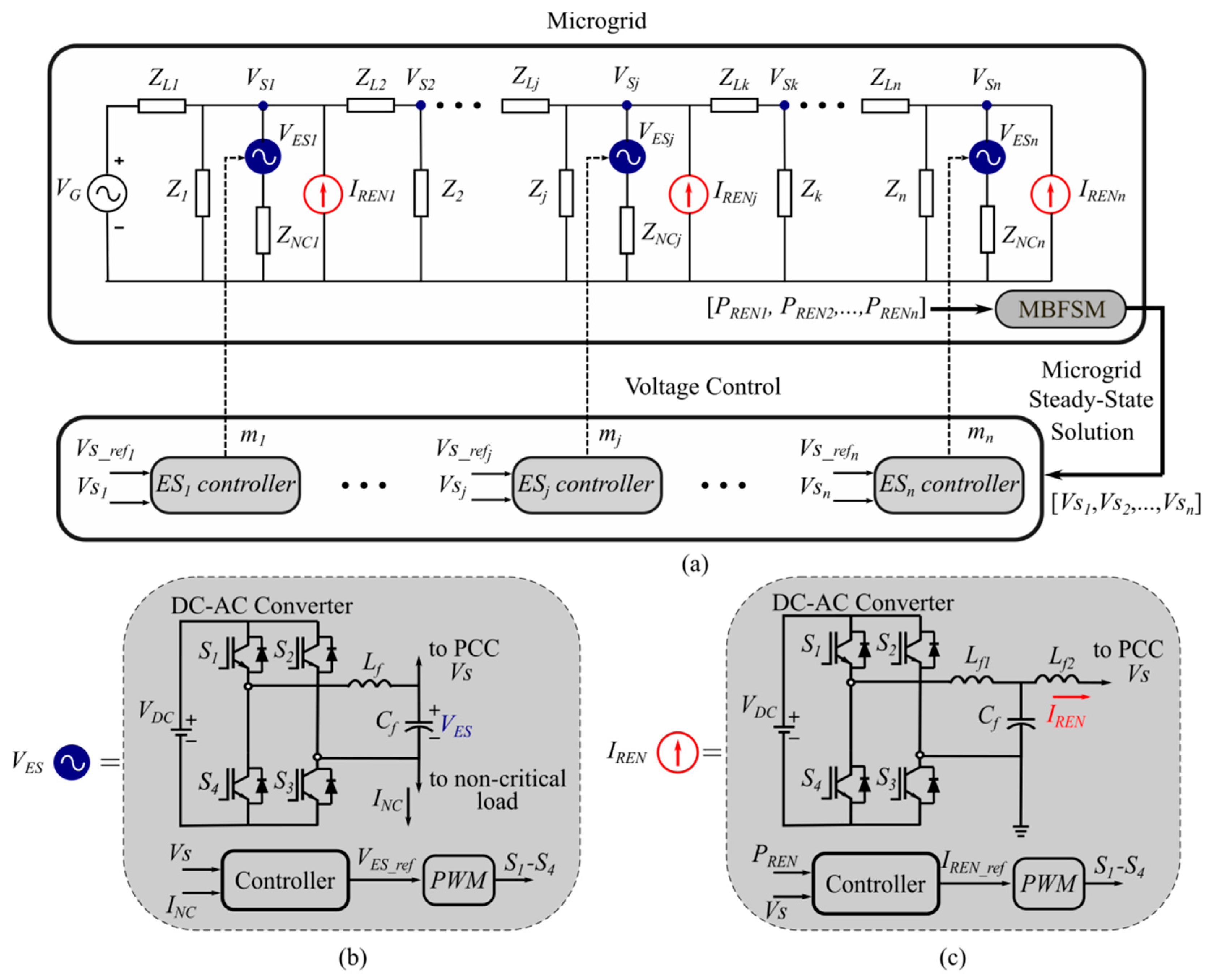
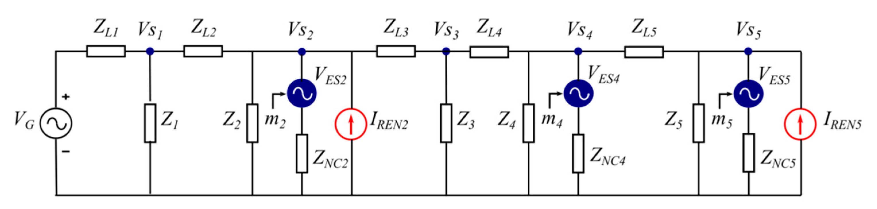
The steady-state model consists of three main stages, which are the µG, the MBFSM algorithm, and the voltage control algorithm, as shown in Figure 3a. The µG has a radial topology, which is one of the most used in distribution systems, and this is composed of a voltage source, VG, that represents the utility grid and a set of elements connected through the line impedances (ZL1, ZL2, …, ZLn). The voltages of the µG are numbered sequentially, starting from the closest one to VG until reaching the last node (Vs1, Vs2, …, Vsn). The physical location of an element is given by the subscript number of the node to which it is connected. These two actions allow for the homogenizing of the information and for the identifying of the elements that compound the µG. The µG contains critical loads (Z1, Z2, …, Zn) and non-critical loads (ZNC1, ZNC2, …, ZNCn). The critical loads are shunt connected with the SLs, and non-critical loads are series connected with the ESs. The DG is represented employing a set of current sources (IREN1, IREN2, …, IRENn), where the subscript 
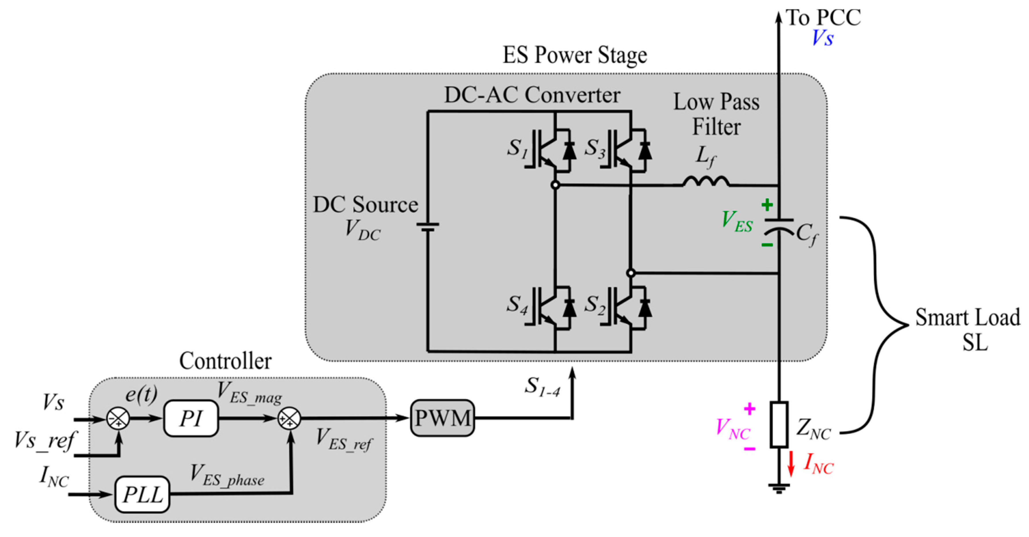
REN means renewable energies. The ESs are modeled as a controlled voltage sources (VES1, VES2, …, VESn) which modify their voltages based on their control variables (m1, m2, …, mn).
The steady-state solution of the µG is obtained using the MBFSM algorithm. The algorithm receives as input the operating conditions of the ESs (m1, m2, …, mn), and the active power injected by each of the RESs (PREN1, PREN2, …, PRENn). In each iteration, the currents delivered by the current sources are calculated by Equation (7) to inject active power only.
I R E N x = P R E N x V s x ,
where the subscript x is associated with the physical location of the current source and takes the values x = 1, 2, …, n, when the MBFWM algorithm converges and the steady-state solution is obtained. An additional algorithm is in charge of controlling the voltage of each ES. The voltage control algorithm receives as input the steady-state solution calculated by the MBFSM and adjusts the operating conditions of the ESs until reaching the reference voltages (Vs_ref1, Vs_ref2, …, Vs_refn).
The validation of the proposed model is carried out by comparing the obtained results with the ones obtained by the solution in the steady-state condition of the time-domain-based model for the µG under the same operating conditions. For the time-domain simulation, the ES is implemented by using its dynamic model (see Figure 3b). At the same time, the current sources associated with the DG are replaced by the dynamic model depicted in Figure 3c. Each current source consists of a DC-AC converter and a low-pass filter (Lf1-Cf-Lf2), operating as a controlled current source. The magnitude and phase for the current signal are calculated from the delivered active power and the voltage in the PCC.

3.1. Steady-State ES Mathematical Model

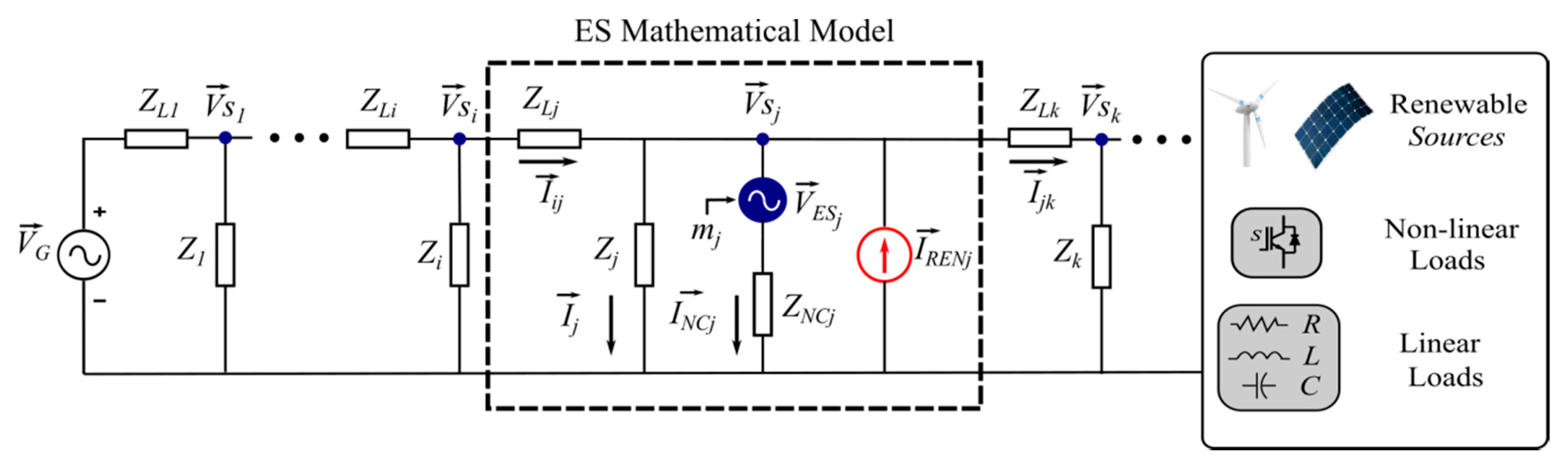
The dotted rectangle in Figure 4 contains the elements and variables involved in the derivation of the ES mathematical model. This part corresponds to a general section of the circuit shown in Figure 3a. There are three nodes involved in obtaining the model, which are indicated by different subscripts (i, j, and k). The subscript j represents the physical location of the ES, while i and k are used to indicate the neighboring nodes. The current contributions of all the elements connected to the PCC, V s j , are considered. It can be seen that the components connected to V s j are those that are usually included in the steady-state models, e.g., the critical loads Zj and the SL. To increase the robustness of the model, the injection of active power into the PCC, I R E N j , and the effect of external disturbances associated with voltage variations, V s i , and current fluctuations I j k are included. V s i in the model involves the voltage variations attributed to V G or the power variations at nodes that precede the location of the ES, and the impact on its operation. I j k corresponds to the current demanded by either the loads or other elements connected in the µG. On the other hand, when I j k is included, the effect of power variations on the rest of the network and the impact that they have on the operation of the ES are also included in the model.
A steady-state analysis is performed on the elements found within the dotted rectangle in Figure 4 to obtain the ESs mathematical model. By applying Kirchhoff’s Voltage Law (KVL) between V s i and V s j , the following equation is obtained.
V s i = I i j Z L j + V s j
where I i j is the current that flows through the distribution line impedance, ZLj. Applying a Kirchhoff’s Current Law (KLC) at the node V s j , the following expression is obtained,
I i j = I j + I N C j I R E N j + I j k ,
where I j , I N C j , …, and I j k correspond to the currents in the critical load, non-critical load, the current delivered by the RESs, and the current demanded by other elements of the µG. The current I j is expressed in terms of the voltage V s j and the impedance Zj as follows:
I j = V s j Z j .
By substituting Equations (9) and (10) in Equation (8), it is obtained that:
V s i = V s j [ Z L j Z j + 1 ] + Z L j I N C j Z L j I R E N j + Z L j I j k .
Expressing the active power delivered for the renewable energy source, PRENj, in terms of V s j and ( I R E N j ) * in polar form, it results that:
P R E N j = V s j ( I R E N j ) * = ( V s j θ s j ) ( I R E N j θ s j ) ,
where θsj is the phase angle of V s j and ( I R E N j ) * is the conjugated of the current I R E N j .
From Equation (12), I R E N j can be represented in terms of the phasor V s j as given in Equation (13)
I R E N j = I R E N j θ s j = P R E N V s j 2 V s j .
Equations (14) and (15) give the V s j and I j k phasors represented in polar form, respectively.
V s j = V s j θ s j ,
I j k = I j k θ j k ,
where θjk is the phase angle of the current I j k .
Defining α = θsjθjk, then I j k can be expressed in terms of V s j as shown in Equation (16)
I j k = ( I j k V s j θ j k θ s j ) ( V s j θ s j ) = ( I j k V s j α ) V s j .
Substituting Equations (13) and (16) in Equation (11), it results:
V s i = V s j [ 1 + Z L j Z j + Z L j I j k V s j α Z L j P R E N V s j 2 ] + Z L j I N C j .
Now, defining V G 1 as follows:
V G 1 = V s j [ 1 + Z L j Z j + Z L j I j k V s j α Z L j P R E N V s j 2 ] ,
equations can be expressed in a compact form by:
V s i = V G 1 + Z L j I N C j .
Additionally, by applying a KVL in the V s j node, the equation associated with the SL is given by:
V s j = V E S j + I N C j Z N C j .
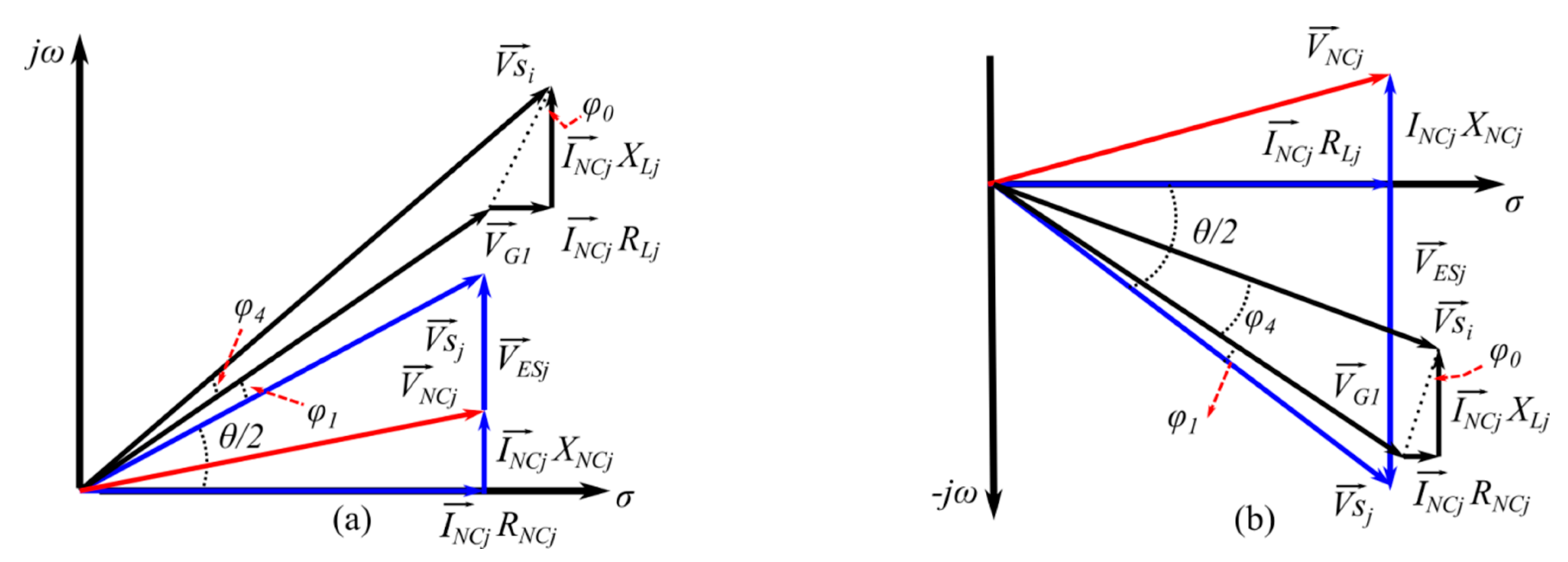
Unlike other works, the proposed model and the calculation of geometric relationships among the electrical variables of the ES consider the load contributions in the PCC and the current contributions associated with external disturbances, as was shown in the approach to derive Equations (19) and (20). This model, unlike the one reported in [23], is not obtained from an equivalent circuit of the electrical network, which increases its robustness. The geometric relationships of the model described in Equations (19) and (20) are illustrated in Figure 5a,b. The phasors represent the Equation (19) in black color. This equation considers the voltage drop in ZLj produced by the current I N C j . This voltage drop is divided into two components related to the resistance, RLj, and reactance, XLj of ZLj. The other term involves V G 1 , whose magnitude and phase are influenced by different parameters, as shown in Equation (18).
On the other hand, Equation (20) is represented for the blue color phasors in Figure 5a,b. One term represents the voltage drop across the non-critical load V N C j , having two components associated with the resistance, RNCj, and reactance, XNCj of ZNCj, and the other term is linked with the ES operation mode. In inductive operation mode V E S j is lagging I N C j by 90o degrees, as shown in Figure 5a. In capacitive operation mode, V E S j it is leading I N C j by 90o, as shown in Figure 5b. The geometric relationships involve four angles. The angle φ 1 is measured from V s j to V G 1 , and the angle φ 0 is associated with the power factor of ZLj. The angle φ 4 is measured from V G 1 to V s i , and finally, θ / 2 is the angle between I N C j and V s j .
When performing the analysis of the geometric relationships of the phasor diagrams in Figure 5,b, the mathematical model described by the next Equations (21)–(29) is obtained. This model differs from that reported in [23] in the calculation of VG1 and φ 1 , while the rest of the geometric relationships remain unchanged. This fact is closely linked with the procedure to derive Equations (13) and (16), which allowed finding a connection between V G 1 and V s j . As a result, a model like the one expressed in Equations (19) and (20) is obtained.
It can be seen in Equations (21) and (22) that the magnitude of VG1 and φ 1 depend on the impedances connected to the PCC (ZLj and Zj), the active power, PRENj, the magnitude of the current Ijk, the magnitude of the voltage on the PCC, Vsj, and the angle α. Variations of any of these parameters will influence the calculation of their geometric relationships. Therefore, the modeling and implementation of the µG in simulation is not a trivial task. However, the BFSM provides an advantage in the implementation of the ES mathematical model. As previously mentioned, this solution technique starts at the node farthest from the µG and, employing the backward propagation, the voltages and currents are calculated until reaching the power supply. This advantage provided by BFSM allows the ES model to be implemented in any µG location without the need for additional restrictions. For instance, to calculate the geometric relationships of an ES connected to the PCC at node Vsj, the BFSM provides the values of V s j and I j k . The rest of the terms are parameters and operating conditions of the PCC, which are known.
V G 1 = | 1 + Z L j Z j + Z L j I j k V s j α Z L j P R E N j V s j 2 | V s j .
φ 1 = arg ( 1 + Z L j Z j + Z L j I j k V s j α Z L j P R E N j V s j 2 ) .
The angle φ 0 depends on the power factor of ZLj as follows:
φ 0 = arg ( Z L j ) .
The ES operating conditions are defined by the parameter mj, and this parameter takes values in the range of [−1, 1] and determines the magnitude of Vsi and the angle θ according to the following relationships.
V s i = m j a 2 + b 2 + V G 1 2 + b .
θ = sin 1 ( m j ) tan 1 ( b a ) .
The parameters a and b are used to simplify Equations (24) and (25). They are given by:
a = V G 1 V s j R N C j R L j 2 + X L j 2 cos ( φ 0 + φ 1 ) .
b = V s j 2 ( R L j 2 + X L j 2 ) 2 R N C j 2 + V G 1 V s j R N C j R L j 2 + X L j 2 sin ( φ 0 + φ 1 ) .
The magnitude of the ES voltage is calculated by Equation (28). If the non-critical load has a unity power factor, the second term of the equation is omitted. If it has a lagging power factor, the sign is negative, and if it is leading, the sign is positive.
V E S j = V s j sin ( θ 2 ) ± I 3 X N C j .
The angle φ 4 is calculated by Equation (29)
φ 4 = sin 1 ( V s j R j 2 + X j 2 R N C j V s i cos ( θ 2 ) cos ( θ 2 + φ 0 + φ 1 ) ) .
It can be seen in Figure 5a,b that the geometric relationships take as reference the phasor I N C j . The reference was established to simplify the calculation of geometric relationships. However, it is necessary to calculate the exact value of the phase angle for the ES voltage, θESj. This value is obtained by the Equation (30) and is calculated from θSj. The value of θSj is provided by the MBFSM in the backward propagation process. If the angle θ takes a positive value, the ES operates in inductive mode; while for a negative value, the operating mode is capacitive.
θ E S j = θ s j θ 2 + s i g n ( θ ) π 2 .
In the same way, the phase angle for the voltage Vsi, θsi is calculated taking as reference θSj in the next equation.
θ s i = θ s j + φ 1 + φ 4 .
Finally, to calculate the current and continue with the backward propagation process, Equation (9) is used. The geometric relationships described in Equations (21)–(31), along with the MBFSM solution technique, allow analyzing the joint operation of RES and ESs distributed in the µG. MBFSM is an iterative process that calculates the steady-state solution of the µG until it converges or reaches a maximum number of iterations. The following subsection describes in detail the implementation of the solution algorithm and the proposed modification to the traditional BFSM.

3.2. Modified Backward–Forward Sweep Method

The BFSM has been extensively used for the steady-state solution of radial electric networks due to its accuracy and fast convergence. There are three variants in the method that depends directly on the type of electrical quantities used: (a) the current summation method, (b) the power summation method, and (c) the admittance summation method [
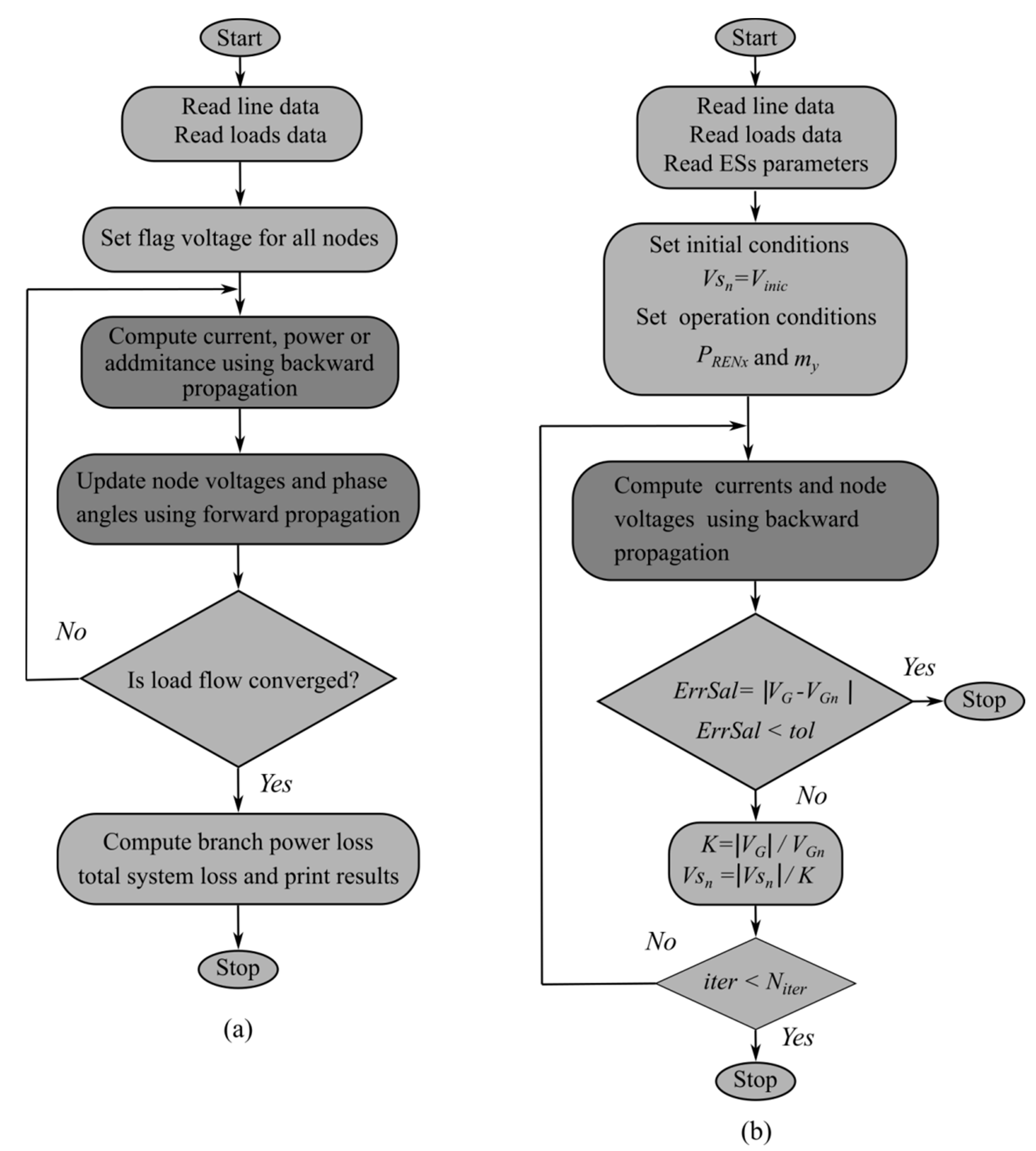
32]. The BFSM procedure is depicted in Figure 6a. It starts with a flat solution in which the voltage at all nodes takes the same value. The backward sweep begins at the farthest node of the radial grid and moves toward the source node computing the currents or power flow in each branch. The forward sweep computes the voltage drop in the electrical grid from the currents or power flows calculated in the backward sweep. The nodal voltages are updated from the voltage source to the last node of the electric grid. During the forward sweep process, the currents or powers calculated in the backward sweep remains constant. The values calculated in the forward sweep correspond to the new voltage values used in the backward sweep for the next iteration. The convergence is reached when the mismatch voltage is less than the specified tolerance.
In this work, it is proposed to modify the traditional BFSM algorithm eliminating the forward propagation process. In general, two factors benefit the proposal and make its implementation viable. The first one is that in the backward propagation, the algorithm simultaneously calculates the currents and voltages at each node. The second one is associated with the proposed ES model, which was designed to operate in conjunction with the solution method. As was seen in the previous section, the model calculates the magnitudes and phase angles at both the PCC and the node that precedes it from the ES operating condition defined by the parameter mj. Therefore, it is possible to simultaneously calculate the currents and voltages at the nodes where the ESs are physically located, avoiding the need to implement the forward propagation step.
Figure 6b shows the flowchart for the MBFSM algorithm proposed in this work. This algorithm computes the solution for the proposed model (see Figure 3a). The algorithm begins with the reading of the parameters (lines, load, and ESs) that conform to a µG. Then, the active power delivered by the current sources (PREN1, PREN2, …, PRENx) and the operation conditions of the ESs (m1, m2, …, my) are established. It is worth noting that different subscripts are used in order to generate a complete scenario; for instance, the subscripts x and y are used to indicate that the number of ESs and RES located in the µG may be different and not necessarily be equal to the number of nodes in the µG established by the subscript n. The initial condition of the farthest voltage in the µG is assigned, Vsn. It can be seen from the flowchart in Figure 6b that forward propagation is omitted because, in the backward propagation, the currents and node voltages are simultaneously calculated until reaching the power supply, VG. If a node, where an ES is located, is reached during the backward propagation process, the model presented in Equations (21)–(31) is employed to calculate the geometric relationships of the electrical quantities in the PCC. As the voltage VG calculated in the backward propagation may not correspond to the real voltage of the power supply, VGn, the output error, ErrSal, is calculated as the absolute value of the difference between VG and VGn. If ErrSal is less than a tolerance, tol, the algorithm stops. The value assigned to tol directly impacts the accuracy of the solution and execution time. The tuning of this parameter must be carefully done as it depends on the dimensions of the µG and the number of ESs and RESs. In this work, a value of tol = 1 × 10⁻¹² was used, which was determined through an exhaustive experimentation. If the condition is not met, a new value of Vsn is calculated for the next iteration. The new value of Vsn is calculated by dividing the current value by an adjustment gain, K. The gain K is calculated by the ratio of the absolute value of VG and VGn. The process is repeated until the maximum number of iterations, Niter, is reached, or the algorithm converges.
The MBFSM accurately provides the steady-state solution of the µG. This solution is calculated from the operating conditions of the ESs and the active power injected by each of the RES; therefore, it is possible to study the impact that DG has on µG. Another area of opportunity for the proposal is provided by the ability to establish the operating conditions of the ESs. These features allow analyzing the individual or joint operation of the ESs and developing global control schemes that face the challenges of modern electric power networks. In this sense, the following subsection explains in detail the voltage control scheme proposed in this work, which is in charge of regulating the operating conditions of multiple ESs distributed in the µG.

3.3. Voltage Control Algorithm Applied to Multiple ESs

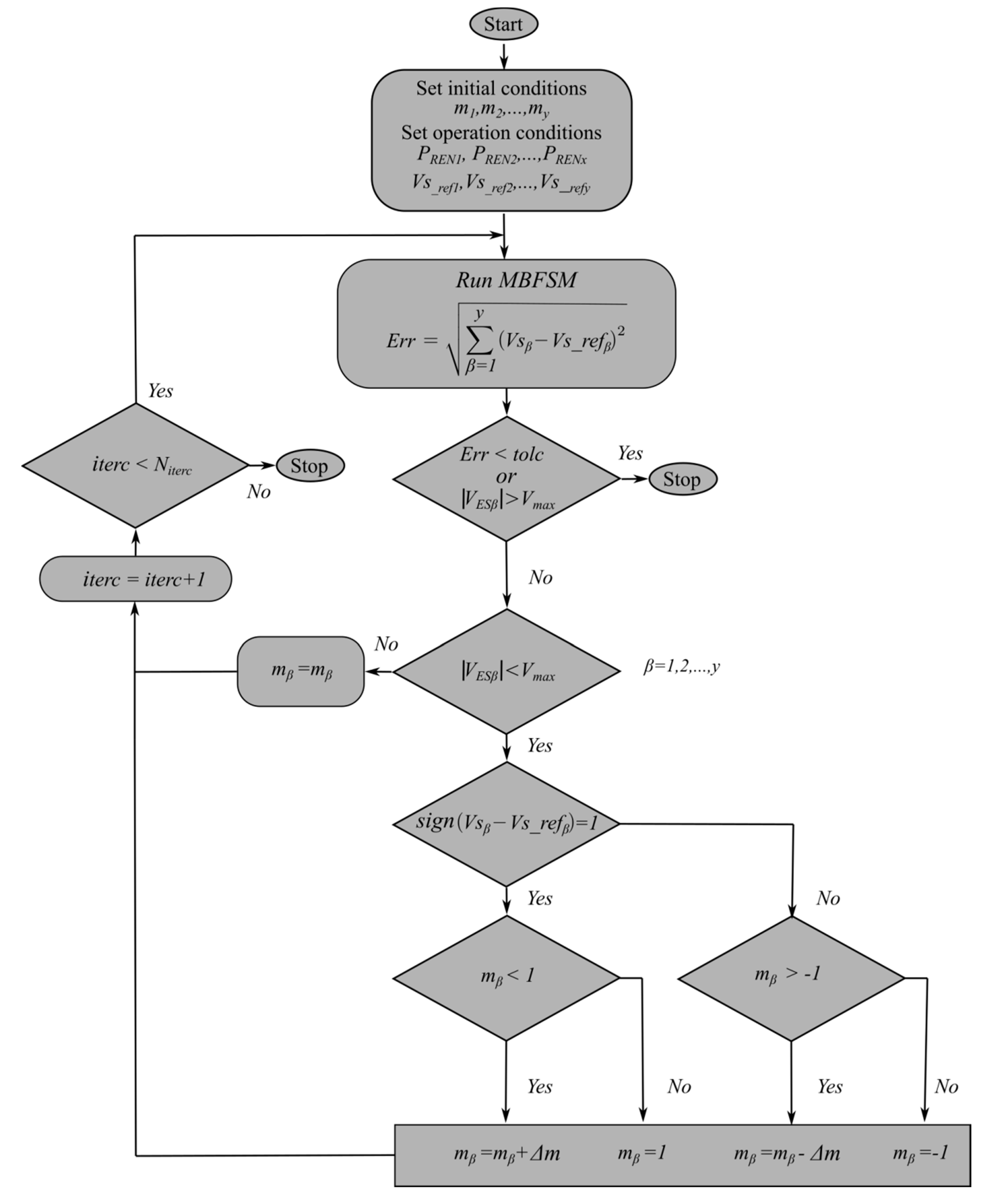
Figure 7 depicts the flowchart for the voltage control algorithm of a group of ESs distributed in the electric grid. This algorithm controls the interaction of all the elements in Figure 3a. The algorithm starts by initializing the operation conditions of all the ESs (m1, m2, …, my) and their respective reference voltage (Vs_ref1, Vs_ref2,…, Vs_refy). The magnitude of the active powers supplied for the current sources are established, which are kept constant until the algorithm converges (PREN1, PREN2, …, PRENx). The algorithm computes the steady-state solution of the µG in each iteration using the MBFSM. Only the voltages of the nodes where the ESs are located are extracted from the steady-state solution (Vs1, Vs2, …, Vsy).
The root mean square error, Err, is calculated from the Vsβ and Vs_refβ, where β =1,2, …, y. If Err is less than the tolerance, tolc, or the voltage magnitude of all ESs reaches its maximum value, Vmax, then the algorithm stops. Vmax is directly related to the magnitude of the voltage source on the DC bus. In one case of the two previous conditions is not fulfilled, it is necessary to modify the operating conditions of each one of the ESs. The following procedure applies to each situation individually. The ESs that reached their Vmax are identified, and their mβ are not modified in this iteration. For the ESs that did not reach Vmax, the sign is obtained from the subtraction (VsβVs_refβ). If the sign is positive, it means that the voltage Vsβ is higher than Vs_refβ; therefore, it is necessary to consume a higher amount of reactive power to decrease the voltage at node Vsβ, which is achieved by increasing mβ, having as a limit a maximum value of 1. Otherwise, mβ must be reduced to a minimum value of −1. This action is associated with an increment in the reactive power injected by the ES. The process is repeated until the solution converges or the maximum number of iterations has been reached.
Once the µG voltage control and the solution algorithms have been implemented, it is necessary to validate the ES model under different operating conditions. In the next section, the obtained results for the proposal are presented.

4. Study Cases and Results

Figure 8 shows the µG implemented to carry out the model validation. It can be seen that it has the topology shown in Figure 3. The assignment of subscripts in the elements corresponds to the criteria described in Section 3. The µG is composed of a power supply, VG, five distribution lines (ZL1, ZL2, ZL3, ZL4, and ZL5), three ESs (ES2, ES4, and ES5), two RES (IREN2 and IREN5) with powers (PREN2 and PREN5), three non-critical loads (ZNC2, ZNC4, and ZNC5), and five loads (Z1, Z2, Z3, Z4, and Z5), where Z2, Z4, and Z5 are the critical loads. The five node voltages are indicated as (Vs1, Vs2, Vs3, Vs4, and Vs5). Table 1 shows the numerical values for the elements that integrate the µG, and these parameters are similar to the ones used in other works to study the impact of the ESs in the µGs [33].
For the implementation of the dynamic simulation model, each ES has its control and has no communication with other ESs. The control has a PLL to operate in reactive power compensation mode and a PI controller to regulate the magnitude and operation mode of the ESs (see Figure 3b). For each IREN, a PLL is used to maintain the injected current in phase with the voltage to deliver active power only (see Figure 3c). The controllers’ gains were adjusted experimentally using the best transient response as the fit criterion. The obtained gains are shown in Table 2.
In the next subsections, the study cases carried out to demonstrate the usefulness and effectiveness of the proposed method are shown. They are all developed using MATLAB software. It is worth noting that the setpoints adjustment of the ESs and the variation in the power injection of the RES are the scenarios that mostly occur in the operation of a µG with DG and distributed ESs; therefore, their study is fundamental (study cases 1 and 2). For validation purposes, the µG time-domain model is implemented, which includes the dynamics of the power and control stages of the ESs. These dynamic models represent an adequate point of comparison since they have been exhaustively studied in different publications reported in the literature [19,20,26,29]. The results obtained when the dynamic model reaches its steady state are the criteria used to carry out the validation; therefore, aspects related to transitory response are not considered in the discussion of the results. Finally, the performance of the model and control algorithms for the implementation of a quasi-stationary study case is presented (study case 3). It provides a handy tool to explore operating scenarios where the transient behavior does not play an important role. As a result, more extended operating scenarios can be implemented with the active participation of more devices and with less computational effort compared to dynamic simulation models.
In order to quantitively evaluate the performance of the MBFSM against the BFSM, a study case with different operating conditions is implemented. The µG of Figure 8 and the parameters of Table 1 are used. A set of n = 100 random values given by xj are generated for the powers injected by the RES (PREN2 and PREN5). The active power is in the range of 0 to 1000 W, which corresponds to the maximum and minimum values used in the next study cases of Section 4.1 and Section 4.2. These arrays are mathematically represented by Equation (32). In the same way, 100 random values are generated for the operating conditions of the ESs. (m2, m4 y m5). These values are contained in the range [−1, 1], which allows the ESs to operate in inductive or capacitive compensation mode. The mathematical representation of these arrays is shown in Equation (33).
P R E N i n = { [ x 1 ; x 2 ; ; x n ] } x j , j = 1 , 2 , , n x j [ 0 , 1000 ] W i = 2 , 5.
m i n = { [ x 1 ; x 2 ; ; x n ] } x j , j = 1 , 2 , , n x j [ 1 , 1 ] i = 2 , 4 , 5
The convergence criterion used in the BFSM is defined by Equations (34)–(36) [34]. The voltage errors (ΔVi) for all nodes in the electrical network are calculated from the voltages in the current iteration (k) and the previous iteration (k − 1), as shown in Equation (34). A convergence error (err) is defined. If Equations (35) and (36) are satisfied for all nodes, the method stops, and the steady-state solution is obtained.
Δ V i = V s i k V s i k 1 i = 1 , 2 , , n
| r e a l ( Δ V i ) | < e r r i = 1 , 2 , , n
| i m a g ( Δ V i ) | < e r r i = 1 , 2 , , n
The convergence criterion implemented for the MBFSM differs from that used in the BFSM. This criterion has been extensively discussed in Section 3.2 and is represented by:
| V G V G n | < e r r
Table 3 contains the results obtained for different convergence errors. The smallest convergence error is 1 × 10⁻¹, and the maximum one is 1 × 10⁻¹². For each method, the maximum, minimum, and average iterations are extracted, considering the 100 samples from the test bench. It can be seen that for all the convergence errors analyzed, the MBFSM obtains the solution in a smaller number of iterations, achieving a reduction of 34.9% in all the cases, which demonstrates the improvement in the computational effort when implementing the MBFSM.

4.1. Study Case: Constant Active Power and Changes in Reference Voltages

In this study case, the active power injected by the RES is kept constant, and the reference voltages of the ESs are modified. In this way, the source of the disturbances is fully identified, and the effect that it has on the µG is analyzed. The study case is divided into three time-intervals to show the different operating conditions of the ESs. The duration time of the intervals was determined based on the transient response of the µG. The time to reach the steady state depends on the severity of the disturbance and the collective action of the devices that conform to the µG. Therefore, this time can vary from one interval to another. In order to unify the criteria, it was adjusted to a value of 75 s, which was obtained experimentally. The active power injected by the RESs remains constant at the values PREN1 = PREN2 = 500 W. These values represent approximately 70% of the energy consumed in the µG under nominal conditions. Therefore, it is possible to reduce the power losses and adjust the reference voltages of the ESs to values close to the nominal voltage of the µG.
Figure 9 shows the behavior of the electrical quantities for the nodes Vs2, Vs4, and Vs5, which correspond to the location of the ESs. The results obtained with the proposed steady-state model are identified with the subscript model. On the other hand, the results of the dynamic simulation are presented using root mean squarer values (RMS) and instantaneous values. When it corresponds to an RMS value, the dynamic subscript is added, and when the electric variable corresponds to an instantaneous value, it is indicated with the subscript dynamic_ins.
In the first interval, the reference voltages of the ESs are set to 119 V. It can be seen in Figure 9a that all the ESs reach the established reference voltage (red line). To achieve the objective of controlling the voltages on the Vs2, Vs4, and Vs5 nodes to a value of 119 V, the ESs modify their voltage, reactive power, and operation mode (see Figure 9b,c). It can be seen that all the electrical variables in the dynamic simulation start with zero initial conditions, and after a transient, it reaches the steady state. It is essential to note the differences in the transient duration times for each voltage even though they include a controller with the same gains. These differences are presented because all the elements are interconnected, and the action of one ES affects the others. However, the ES local controller allows the gradual adjustment until the steady state is reached.
Regarding the steady-state model, this effect is already considered in the modeling and is adjusted using the solution and control algorithms. Results calculated with the steady-state model are represented as a constant value throughout the interval (black line). When comparing both results, it is verified that the results obtained by the steady-state model and the dynamic model are the same. From Figure 9b,c in the first interval, it can be seen that (i) ES2 operates in inductive mode with a voltage VES2 = 40.29 V and absorbs a reactive power QES2 = 90.23 VAR, (ii) ES4 also operates in inductive mode but with VES4 = 22.17 V and QES4 = 51.83 VAR, and (iii) ES5 operates in capacitive mode, delivering a reactive power QES5 = −106.5 VAR and a voltage VES5 = 49.12 V.
The second interval shows the performance of the control algorithm when the ESs operate under saturation conditions. This effect occurs when the limits of voltage in the DC bus for the ES are exceeded. Regarding dynamic simulation, this limit is established by the element that powered the DC bus. If the required control action is higher than its limit, the ES voltage is adjusted to the maximum value and remains constant. If this restriction is not included in the steady-state model, the calculated ESs voltage will be wrong, and the collaborative operation of the ESs will not be appropriately modeled. In this regard, the reference voltage of the ES2 changes to Vs_ref2 = 121 V, and the voltages of the other two ESs remain constant at Vs_ref4 = 119 V and Vs_ref5 = 119 V. The new value of Vs_ref2 affects the entire µG causing changes in the voltages and modes of operation of the ESs since they try to reach their established reference voltage. Only Vs5 reaches 119 V, while the other voltages are controlled at the values, Vs4 = 119.2 V and Vs2 = 120.5 V. The modification in Vs_ref2 causes the change in the operation of the ES from inductive mode to a capacitive mode in order to increase the voltage in its PCC. However, it reaches its maximum voltage VES2 = 70.71 V and delivers a reactive power QES2 = −137.9 VAR. The maximum voltage of the ESs is restricted by the voltage source that powered the DC bus. In this study case, it has a value of 100 V, and it is indicated in Figure 9b. The ES4 also reaches its maximum voltage VES4 = 70.71 V, but it operates in inductive mode, consuming a reactive power QES4 = 135.7 VAR. The ES5 is kept in capacitive mode with a voltage VES5 = 29.7 V and a reactive power QES5 = −68.45 VAR.
As was seen in the second interval, the modification in the reference voltage of one ES directly affects the other ESs. It is possible that in some cases, the ES reaches its operating limits, which is not adequate since this condition will not allow the appropriate handling of the power intermittencies in the µG. Therefore, it is essential to show that an increment or decrement of voltage is a collective task of the ESs, which is directly related to the assignment of the reference voltages of the ESs. At this point, the collaborative action is fundamental since if the reference voltages are arbitrarily adjusted, the ESs will have a conflict to establish their set points. This fact sometimes puts the ESs in saturation mode, resulting in an inadequate energy management which will directly impact on the µG’s voltage regulation and, consequently, its reliability.
Finally, in the third interval, the reference voltages are adjusted to the values Vs_ref2 = 122 V, Vs_ref4 = 122.5 V, and Vs_ref5 = 122 V. In this interval, none of the ESs reaches their maximum voltage, allowing the voltage control at the nodes Vs2, Vs4, and Vs5 with their reference voltages, respectively. The ES2 remains in capacitive mode with voltage and reactive power VES2 = 63.51 V and QES2 = −132.3 VAR, respectively. The ES4 operates in capacitive mode, and its voltage and reactive power are VES4 = 50.31 V and QES4 = −112.4 VAR, respectively. The ES5 operates in inductive mode with a voltage and reactive power VES5 = 1.695V and QES5 = 4.112 VAR, respectively.
The results presented in this study case were allowed to validate the ES model and the proposed algorithms subjected to modifications in their reference voltages. The steady-state comparison of both simulation models showed the same results in the three simulation intervals; however, the computational effort for the dynamic simulation model is higher because it is necessary to compute the transient response to get the steady-state. The proposed model and the algorithms for its solution and control described the collective operation of multiple ESs in µGs adequately. The tests carried out properly showed the action in reactive power compensation mode and the saturation effect on the ESs.

4.2. Study Case: Constant Reference Voltages and Changes in ACTIVE POwer

In this case study, the reference voltages of the ESs are kept constant throughout the simulation, while the powers of PREN2 and PREN5 are modified. The purpose of this study case is to validate the model when it is subject to power disturbances, which is one of the most critical requirements in µGs with DG. The study case is divided into three intervals of 75 s. The values that PREN2 takes in each interval is 500 W, 500 W, and 1000 W, while PREN5 takes the values 0 W, 500 W, and 1000W. These values represent 35%, 70%, and 140% of the power consumed by the loads in nominal operating conditions. Therefore, the study case will allow observing the power handling of the ESs when there is a lack of dispatch (intervals 1 and 2) or surpluses of power (interval 3). The obtained results allowed demonstrating the proper operation of the proposal to manage power intermittencies and support voltage regulation locally simultaneously. The reference voltage of the ESs is adjusted to a fixed value Vs_ref2 = Vs_ref4 = Vs_ref5 = 120V, which is determined based on the nominal voltage of the µG power supply.
Figure 10a shows the voltages at the nodes Vs2, Vs4, and Vs5. It can be seen that Vs2 and Vs4 are controlled at 120 V established by their reference voltages, regardless of the disturbances produced by the RES. On the other hand, Vs5 in the first interval reaches a value of 119.7 V (maximum allowed voltage), and in the following two ranges, it reaches the reference voltage of 120 V. The voltages obtained in the dynamic simulation show a transient at the beginning of each time interval, and later the steady state is reached.
The power disturbances produced in each interval cause the adjustment of the voltages and the operation modes of the ESs since the voltages in each PCC have to be controlled (see Figure 10b,c). During the first interval, the ESs operate in capacitive mode since the active power provided by PREN2 = 500 W is not enough to compensate for the voltage drops in the µG. Consequently, the ESs operate in capacitive mode to increase the voltage in their respective PCC. In this interval, the voltages of the ESs are VES2 = 23.04 V, VES4 = 4.541 V, and VES5 = 70.71 V, and the reactive powers are QES2 = −54.27 VAR, QES4 = −10.89 VAR, and QES5 = −136.6 VAR. On the other hand, in the second time interval, the active power increases to the values PREN2 = 500 W and PREN5 = 500 W. The increment in the delivered active power reduces the voltage drops in the µG, causing a reduction in the amount of reactive power delivered by the ESs. The ES2 and ES5 keep operating in capacitive mode, but now the voltages are modified to the values VES2 = 2.236 V and VES5 = 50.36 V, while the reactive powers are adjusted to QES2 = −5.58 VAR and QES5 = −109.7 VAR. Regarding the ES4, it changed its operation mode to inductive mode with a voltage VES4 = 22.53 V and a reactive power QES4 = 53.11 VAR.
In the last interval, the total active power increases to 2000 W, distributed equally between PREN2 and PREN5, so this causes an increment in the node voltages and, consequently, the reactive power exchanged between the ESs and µG is modified. The ES2 and ES4 change their operating mode to inductive mode, and the ES5 decreases the amount of reactive power delivered. The new voltages at which the ESs operate are VES2 = 26.24 V, VES4 = 13.34 V, and VES5 = 7.318 V, and the reactive powers are QES2 = 61.44 V, QES4 = 15.51 VAR, and QES5 = −17.53 VAR.
The results obtained with the steady-state model are equal to the ones obtained with the time-domain model, demonstrating that the model is valid to adequately and accurately represent the behavior of the multiple ESs under power disturbances. As identical results are obtained, the proposed model can be used and implemented to study large-scale systems with more extended operating scenarios and fewer computational efforts compared with the dynamic simulation models. An important aspect to highlight is the modification of the operating mode in the ESs when the active power increases. This fact is closely linked with his excellent ability to handle power locally. When the active power generated is lesser than the one consumed, the ESs operate in capacitive mode to support the voltage. On the contrary, when the generated power is higher than the one consumed, the ESs absorb reactive power and, consequently, the voltage is decreased.

4.3. Quasi-Stationary Simulation Model with Distributed Renewable Generation

This section implements a quasi-stationary study case. The study case allows for observing the correct performance of the proposal to implement more extended operating scenarios and with different operating conditions of the ESs and RESs distributed in the µG. A quasi-stationary study case with a variable power injection from the RESs with a duration time of 14 h and step increments of one minute is performed. PREN2 and PREN5 are modeled using a gaussian photovoltaic generation curve with a maximum power of 1000 W that occurs at 12 h in both cases. Two disturbances are implemented simulating the effect of shading on the photovoltaic panels. The disturbance affecting PREN5 is a sudden power drop of 300 W that occurs in the interval from 10 to 11 h. The disturbance of PREN2 is of magnitude 500 W, and it occurs in the interval from 12 to 13 h. In both disturbances, a time of 1 h was used to make more evident and clearly show the behavior of the ESs in the management of sudden power changes. Figure 11a shows PREN2 and PREN5. In Figure 11b, the behavior of the five voltages of the µG is shown. Figure 11c,d correspond to the voltages and reactive powers of the three ESs installed.
The power delivered by the RES before the 5 h and after the 18 h is zero, causing the voltages to remain constant with values Vs1 = 119.95 V, Vs2 = 119.88 V, Vs3 = 119.6818, Vs4 = 120 V, and Vs5 = 119.72. This is obtained because the ES2 and ES5 reach their maximum voltage limits, i.e., VES2 = VES5 = 70.71 V operating in capacitive mode with a reactive power of QES2 = QES4 = −136.6 VARs. The Vs4 voltage is the only one that is maintained at 120 V with a VES4 = 8543 V and a reactive power QES4 = −20.45 VAR. This fact is due to that it did not reach its maximum allowable voltage for these operating conditions. As the power of PREN2 and PREN5 increase, the power losses in the distribution lines decrease, causing Vs2 and Vs5 to reach the 120 V reference at t = 7 h and t = 9 h, respectively, and, simultaneously, both ESs leave the operation in maximum reactive power compensation. It can be seen from 9 to 15 h that the voltages Vs2, Vs4, and Vs5 remain at 120 V, which is possible because the ESs can mitigate the disturbances produced by the power injection. The first disturbance occurs in the interval from 10 h to 11 h and only affects PREN5. The two ESs most affected by this disturbance are ES4 and ES5 due to the proximity with PREN5. To maintain the voltage at 120 V, the ES4 increases the amount of reactive power consumed, while the ES5 simultaneously increases the amount of reactive power delivered. The second disturbance occurs in the time interval from 12 to 13 h, which is completely mitigated by the ES2. To achieve this, the ES2 decreased the amount of reactive power consumed; in a short time, it operated in capacitive mode. Regarding the voltages Vs1 and Vs3, they are more affected by the disturbances, which are directly reflected in a greater variation in their voltage.
Figure 12 illustrates the behavior for the voltages of the µG with the operation of the ESs (solid line) and without them (dotted line) under the same considerations of active power injection. The voltages of Vs1 are shown in Figure 12a, the voltages of Vs2 in Figure 12b, the voltages of Vs3 in Figure 12c, the voltages of Vs4 in Figure 12d, and finally the voltages of Vs5 in Figure 12e. It is evident that when the ESs are not used, there are more considerable voltage variations, and their behavior is closely related to the power injection curve. On the other hand, by including the ESs, the voltage regulation is improved substantially. To quantify the voltage variations, the gradients Δ1 and Δ2 are calculated. For the calculation of the gradients, the value of 120 V is taken as reference, which corresponds to the nominal voltage of the power supply. The gradient Δ1 is obtained from the difference between the reference voltage and the maximum voltage, while Δ2 is calculated with the difference between the reference voltage and the minimum voltage. The gradients are graphically indicated in the voltages of Figure 12a–e, and their numerical values are concentrated in Table 4. The shaded area contains the voltages of the µG when the ESs are included. These voltages are zoomed for a better appreciation.
A negative gradient means that the maximum voltage exceeds the reference voltage, while a positive gradient indicates that the minimum voltage is below the reference. For a better context of the results, the gradients calculated without the ESs are first discussed. Column 1 in Table 4 shows the values of Δ1, which are negative and maintain a trend of increasing its value until reaching Δ1 = −0.1660 V, which corresponds to Vs3. Then, the gradients of Vs4 and Vs5 decrease to the values Δ1 = −0.6166 V and Δ1 = −0.5413 V, respectively. This alteration in the trend is closely linked with the injection of active power in Vs2 and Vs5, which decreases the voltage drop in the µG and, consequently, increases the voltage in the farthest nodes. Regarding Δ2 values, they are all positive, showing a continuous magnitude increment as it moves away from the power supply. This behavior is originated because the minima voltages occur when the active power provided by the RES is zero, i.e., in t = 5 h and t = 19 h, generating a gradual voltage drop and being Vs5 the most affected with a Δ2 =6.5444 V.
Columns 3 and 4 of Table 4 contain the gradients of the voltages when the ESs operate in the µG. The values of Δ1 and Δ2 are zero in Vs4 since, throughout the study case, the ES regulates the voltage to 120 V established by its reference voltage. For its part in Vs2 and Vs5, Δ1 = 0 because it never exceeds 120 V. However, in the intervals where the ESs enter in saturation and, therefore, cannot control the voltage, a lower voltage was obtained, i.e., Δ2 = 0.1098 V and Δ2 = 0.2758 V, respectively. Because there are no ESs in nodes Vs1 and Vs3, a higher variation in voltage is obtained; in all the remaining cases, an improvement on the voltage reduction higher than 95% is obtained. The values obtained for Vs1 are Δ1 = −0.6423 V and Δ2 = 0.0427 V. The voltage in Vs3 never exceeds 120 V, causing both gradients to be positive with values Δ1 = 0.2848 V and Δ2 = 0.4661 V.
The results presented in this study case show the robustness and flexibility of both the proposed model and the solution and control algorithms to simulate a variable power injection. As can be seen, they are a great tool to analyze the operation of multiple ESs together with RES, including the analysis of µGs or large-scale distribution systems with DG. This characteristic also allows the development of collaborative control algorithms for managing a higher density of RES and alleviates the problems associated with intermittent energy sources without affecting the reliability of the µG.

4.4. Quasi-Stationary Simulation Model with Real Power Profiles Data

The injection of active power from more real conditions is an aspect of great importance to evaluate simulation models of electrical networks with DG. In this sense, the model was tested by using the daily and annual power profiles from the National Renewable Energy Laboratory (NREL) database [35]. The database contains the power profiles of approximately 6000 distributed photovoltaic solar plants in the USA. The power profiles have the information of the days included in a year. Each profile provides the active power injected in 5 min time intervals. The profiles allow evaluating the simulation models with DG under different operating conditions, i.e., sunny, partially cloudy, or cloudy days. Figure 13 depicts the results obtained from the simulation model and the real data. Figure 13a shows the active power profiles used by PREN2 and PREN5, respectively. These profiles correspond to the days 50 and 210 of a 50 MVA plant located in Arizona, USA. For the study case, the profiles were adjusted to a nominal power of 1 kVA to operate within the range of the power consumed by the loads in the µG. The power profile of PREN2 describes the behavior of a sunny day in the interval time from 8 to 13 h, and with minimal power disturbances. Afterward, the power profile undergoes power variations of different magnitude and duration. Regarding PREN5, its behavior corresponds to a partially cloudy day with power disturbances of greater severity and duration than those shown by PREN2.
The results presented in Figure 13 retain the same format shown in Figure 11. It can be seen that the behavior of the electrical variables is similar to the ones obtained in the study case of Section 4.3, with differences associated with the new power profiles. Figure 13b shows the behavior of the µGs voltages, which remain constant during the null periods of power injection (before 8 h and after 18 h). In these time intervals, the ES2 and ES4 operate at their maximum voltage (VES2 = VES4 = 70.71 V) and in capacitive mode with reactive powers (QES2 = QES4 = −136.6 VAR), as shown in Figure 13c,d, respectively. On the other hand, Vs4 remains constant throughout the simulation at a value of 120 V, which is closely linked to the fact that the ES4 never enters on saturation. Therefore, it can handle power locally and regulate the voltage in the PCC simultaneously. Active power injection comprises the time interval from 8 to 18 h. In this time interval, the ES2 and ES5 come out of saturation, allowing them to regulate the voltage in their PCC to a value of 120 V. The results presented demonstrate a proper behavior of the model and algorithms with real power profiles, where the ESs manage the power variations through three actions, i.e., the adjustment of their voltage magnitude, operation mode, and the amount of reactive power injected or consumed.

5. Comparative Analysis of Analytical Models for the ES Applied in Electrical Systems

In general, the analytical models for the ES used in electrical network simulations are divided into two groups, which are dynamic models and steady-state models. Table 5 shows the essential characteristics, advantages, and disadvantages of both types of mathematical models. Dynamic models are widely used for studies of transient stability [15], power quality aspects related to short-term variations in electrical quantities [36], and harmonics [37]. These models allow the evaluation of overshoots and response times for the in-test system to assess their performance for different tasks, e.g., regulation purposes or disturbance mitigation, to avoid more severe network problems. Simulation models reported in the literature include the operation of a single ES up to several ESs, and in some cases, the models incorporate RES. These studies have been implemented in distribution power systems, grid-connected µGs, or standalone µGs. The power and control stages in these models are independent, which facilitates the implementation of simulation models with multiple ESs [38]. The power stage includes the physical restrictions of the ES, and the control stage is responsible for operating the ES under its operating principle [26]. However, dynamic simulation models require a high computational cost associated with both the robustness of the model and the small integration step in the solution process.
On the other hand, steady-state simulation models are obtained from phasor solution methods. These models are not suitable for reproducing the transitory phenomena of electrical networks. Still, they are characterized by having a low computational effort compared to dynamic models [39], which is a suitable feature to analyze large systems. The study of a single ES or multiple ESs in conjunction with RES has been carried out in distribution power systems, grid-connected µGs, and standalone µGs. These models are divided into two main groups.
  • The first group is represented by power equations that describe the power exchange of the ES in the PCC; however, they have the constraint of being obtained from a simplified electrical network, indicating that their complexity in the study of multiple ESs will be higher. To adequately describe the behavior of the ESs, the models include additional restrictions related to the characteristics of the network, the physical location of the ES, and their operating limits [24,25,40]. Other alternatives carried out increase the complexity of the model since they include a more significant number of equations [21] or the design of external algorithms that restrict the operation of the ESs within established regions [41,42,43].
  • The second group is called phasor models, and within this group is the proposed work. These models are characterized by providing a detailed representation of the geometric relationships of the electrical variables. Although some works have shown its use in grid-connected µGs by considering only one ES [22,23], the needs of modern power systems require the development of more robust models. In this regard, the proposed work outperforms previous works since it can deal with both grid-connected μGs and standalone μGs by considering single and multiple ESs. On the other hand, unlike reported works that consider simplified electrical networks, the proposed model is obtained from a more realistic electrical network by considering the injection of active power into the PCC and the effect of external disturbances on the behavior of the ES. These considerations increase its robustness, allowing for the obtaining of a generalized model suitable for the operation of multiple ESs without the need for additional restrictions. Consequently, a handy tool is obtained to study the requirements of modern energy networks.

6. Conclusions

In this work, a robust steady-state model for the ES is developed. All the considerations involved in its derivation allowed for the reaching of a generalized representation, making suitable its implementation in any physical location of the µG without additional restrictions. This feature expands its applicability in schemes that involve multiple ESs distributed in a µG. The ES model is solved by the MBFSM that allows for the obtaining of the steady-state solution of a µG with DG from the operating conditions of the ESs and the active power delivered by the RESs. Due to the ES model design and the MBFSM, it was possible to omit the forward propagation stage. This omitted step allows simplifying the solution algorithm and reducing the computational effort. Additionally, a control algorithm is implemented to control the µG voltage from the operating conditions of the ESs. The algorithm demonstrates an excellent performance for the control of multiple ESs operating within their limits or under saturation conditions (maximum available DC voltage). The obtained results allow the validation of both the proposed model and the proposed algorithms for the solution and control tasks since the steady-state results obtained by the proposed model are equal to the ones obtained with the dynamic simulation model when the steady-state is achieved. Results also validate of the proposal effectiveness to face active power variations, changes in the reference voltages of the ESs, and different values of loads at each node. The obtained results show an improvement higher than 95% for voltage control when the ESs are installed in the quasi-stationary simulation model; also, the analysis of quasi-stationary study cases with real active power profiles shows the versatility of the proposal for analyzing real scenarios. On the other hand, the MBFSM reduces the number of iterations by 34% on average compared to the BFSM.
The approach presented in this work forms the basis for future research on the operation of multiple ESs in conjunction with DG, allowing the implementation of collaborative control schemes based on intelligent algorithms that guarantee reliability in modern electrical networks. Additionally, it will be possible to analyze operating scenarios with uncertain information through the implementation of estimators and observers.

Author Contributions

Conceptualization, G.T.-T. and A.G.-P.; methodology, G.T.-T, A.G.-P., and M.V.-R.; validation, G.T.-T., D.G.-L., and D.A.R.-A.; formal analysis, G.T.-T, D.G.-L, M.V.-R., and D.A.R.-A.; funding acquisition, A.G.-P., and M.V.-R.; writing—original draft, review and editing, all the authors. All the authors have read and agreed to the published version of the manuscript.

Funding

This research was funded by the “Consejo Nacional de Ciencia y Tecnología (CONACYT)” under the scholarship 728379.

Conflicts of Interest

The authors declare no conflicts of interest.

Nomenclature

ESElectric SpringϕNCNon-critical Load Angle
SGSmart GridsVESElectric Spring Voltage
DGDistributed GenerationVsVoltage on the PCC
RESRenewable Energy SourcesVNCNon-critical Load Voltage
µGMicrogridVs_refReference Voltage on the PCC
SLSmart LoadVES_magMagnitude of the ES voltage control
PCCPoint of Common CouplingVES_phasePhase Angle of the ES Voltage Control
DCDirect CurrentVES_refES Voltage Control
ACAlternating CurrentINCNon-critical Load Current
BFSMBackward–forward Solution Method V G Voltage Source Phasor
MBFSMModified Backward–forward Solution Method V E S Electric Spring Voltage Phasor
PWMPulse Width Modulation V s Voltage on the PCC Phasor
PIProportional Integral Controller V N C Non-critical Load Voltage Phasor
RResistance I N C Non-critical Load Current Phasor
LInductanceQESES Reactive Power
CCapacitanceQNCNon-critical Load Reactive Power
XReactanceQSLSmart Load Reactive Power
ZCritical Load ImpedancePRENRES Active Power
ZNCNon-critical Load ImpedanceIRENRES Current
ZLDistribution Line ImpedancemES operating condition

References

  1. Tuballa, M.L.; Abundo, M.L. A review of the development of Smart Grid technologies. Renew. Sustain. Energy Rev. 2016, 59, 710–725. [Google Scholar] [CrossRef]
  2. Farmanbar, M.; Parham, K.; Arild, Ø.; Rong, C.A. Widespread review of smart grids towards smart cities. Energies 2019, 12, 4484. [Google Scholar] [CrossRef] [Green Version]
  3. Hossain, M.; Madlool, N.; Rahim, N.; Selvaraj, J.; Pandey, A.; Khan, A.F. Role of smart grid in renewable energy: An overview. Renew. Sustain. Energy Rev. 2016, 60, 1168–1184. [Google Scholar] [CrossRef]
  4. Zhang, X.; Wang, R.; Bao, J. A novel distributed economic model predictive control approach for building air-conditioning systems in microgrids. Mathematics 2018, 6, 60. [Google Scholar] [CrossRef] [Green Version]
  5. Yoldaş, Y.; Önen, A.; Muyeen, S.M.; Vasilakos, A.V.; Alan, I. Enhancing smart grid with microgrids: Challenges and opportunities. Renew. Sustain. Energy Rev. 2017, 72, 205–214. [Google Scholar] [CrossRef]
  6. Jung, S.; Yoon, Y.T.; Huh, J.H. An efficient micro grid optimization theory. Mathematics 2020, 8, 560. [Google Scholar] [CrossRef] [Green Version]
  7. Fang, W.; Liu, H.; Chen, F.; Zheng, H.; Hua, G.; He, W. DG planning in stand-alone microgrid considering stochastic characteristic. J. Eng. 2017, 2017, 1181–1185. [Google Scholar] [CrossRef]
  8. Bizon, N.; Thounthong, P. Energy efficiency and fuel economy of a fuel cell/renewable energy sources hybrid power system with the load-following control of the fueling regulators. Mathematics 2020, 8, 151. [Google Scholar] [CrossRef] [Green Version]
  9. Babazadeh, M.; Nobakhti, A. robust decomposition and structured control of an islanded multi-DG microgrid. IEEE Trans. Smart Grid 2018, 10, 2463–2474. [Google Scholar] [CrossRef]
  10. Aderibole, A.; Zeineldin, H.H.; Al Hosani, M.; El-Saadany, E.F. Demand side management strategy for droop-based autonomous microgrids through voltage reduction. IEEE Trans. Energy Convers. 2019, 34, 878–888. [Google Scholar] [CrossRef]
  11. Hui, S.Y.; Lee, C.K.; Wu, F.F. Electric springs—A New smart grid technology. IEEE Trans. Smart Grid 2012, 3, 1552–1561. [Google Scholar] [CrossRef] [Green Version]
  12. Chen, X.; Hou, Y.; Hui, S.Y.R. Distributed control of multiple electric springs for voltage control in microgrid. IEEE Trans. Smart Grid 2016, 8, 1350–1359. [Google Scholar] [CrossRef]
  13. Chen, J.; Yan, S.; Yang, T.; Tan, S.C.; Hui, S.Y.R.; Hui, R. Practical evaluation of droop and consensus control of distributed electric springs for both voltage and frequency regulation in microgrid. IEEE Trans. Power Electron. 2018, 34, 6947–6959. [Google Scholar] [CrossRef]
  14. Chen, J.; Yan, S.; Hui, S.Y.R. Using consensus control for reactive power sharing of distributed Electric Springs. In Proceedings of the 2017 IEEE Energy Conversion Congress and Exposition in Cincinnati, Cincinnati, OH, USA, 1–5 October 2017; pp. 3741–3746. [Google Scholar]
  15. Akhtar, Z.; Chaudhuri, B.; Hui, S.Y.R. Primary frequency control contribution from smart loads using reactive compensation. IEEE Trans. Smart Grid 2015, 6, 2356–2365. [Google Scholar] [CrossRef] [Green Version]
  16. Chakravorty, D.; Chaudhuri, B.; Hui, S.Y.R. Rapid Frequency response from smart loads in great britain power system. IEEE Trans. Smart Grid 2017, 8, 2160–2169. [Google Scholar] [CrossRef] [Green Version]
  17. Zheng, Y.; Hill, D.J.; Song, Y.; Zhao, J.; Hui, S.Y.R. Optimal electric spring allocation for risk-limiting voltage regulation in distribution systems. IEEE Trans. Power Syst. 2020, 35, 273–283. [Google Scholar] [CrossRef]
  18. Moghbel, M.; Masoum, M.A.S.; Fereidouni, A.; Deilami, S. Optimal sizing, siting and operation of custom power devices with STATCOM and APLC functions for real-time reactive power and network voltage quality control of smart grid. IEEE Trans. Smart Grid 2017, 9, 5564–5575. [Google Scholar] [CrossRef]
  19. Yang, T.; Liu, T.; Chen, J.; Yan, S.; Hui, S.Y.R.; Hui, R. Dynamic modular modeling of smart loads associated with electric springs and control. IEEE Trans. Power Electron. 2018, 33, 10071–10085. [Google Scholar] [CrossRef]
  20. Chaudhuri, N.R.; Lee, C.K.; Chaudhuri, B.; Hui, S.Y.R. Dynamic modeling of electric springs. IEEE Trans. Smart Grid 2014, 5, 2450–2458. [Google Scholar] [CrossRef]
  21. Tan, S.C.; Lee, C.K.; Hui, S.Y. General steady-state analysis and control principle of electric springs with active and reactive power compensations. IEEE Trans. Power Electron. 2012, 28, 3958–3969. [Google Scholar] [CrossRef]
  22. Zou, Y.; Chen, M.Z.Q.; Hu, Y. Steady-state analysis and output voltage minimization based control strategy for electric springs in the smart grid with multiple renewable energy sources. Complexity 2019, 2019, 1–12. [Google Scholar] [CrossRef]
  23. Wang, Q.; Cheng, M.; Chen, Z.; Wang, Z. Steady-state analysis of electric springs with a novel δ control. IEEE Trans. Power Electron. 2015, 30, 7159–7169. [Google Scholar] [CrossRef]
  24. Akhtar, Z.; Chaudhuri, B.; Hui, S.Y.R. Smart loads for voltage control in distribution networks. IEEE Trans. Smart Grid 2015, 8, 1–10. [Google Scholar] [CrossRef] [Green Version]
  25. Askarpour, M.; Aghaei, J.; Boudjadar, J.; Niknam, T. Techno-economic potential gains of electric springs in distribution networks operations. IET Gener. Transm. Distrib. 2020, 14, 98–107. [Google Scholar] [CrossRef]
  26. Khamis, A.K.; Zakzouk, N.E.; Abdelsalam, A.K.; Lotfy, A.A. Decoupled control strategy for electric springs: Dual functionality feature. IEEE Access 2019, 7, 57725–57740. [Google Scholar] [CrossRef]
  27. Wang, M.-H.; Yang, T.; Tan, S.C.; Hui, S.Y.R.; Hui, R. Hybrid electric springs for grid-tied power control and storage reduction in AC microgrids. IEEE Trans. Power Electron. 2018, 34, 3214–3225. [Google Scholar] [CrossRef]
  28. Mok, K.-T.; Wang, M.-H.; Tan, S.C.; Hui, S.Y.R. DC Electric springs—A Technology for stabilizing DC power distribution systems. IEEE Trans. Power Electron. 2016, 32, 1088–1105. [Google Scholar] [CrossRef]
  29. Lee, C.K.; Chaudhuri, B.; Hui, S.Y. Hardware and control implementation of electric springs for stabilizing future smart grid with intermittent renewable energy sources. IEEE J. Emerg. Sel. Top. Power Electron. 2013, 1, 18–27. [Google Scholar] [CrossRef]
  30. Sen, B.; Soni, J.; Panda, S.K. Performance of electric springs with multiple variable loads. In Proceedings of the 2016 IEEE 8th International Power Electronics and Motion Control Conference (IPEMC-ECCE Asia), Hefei, China, 22–26 May 2016; Institute of Electrical and Electronics Engineers (IEEE-USA): Riverside, CA, USA, 2016; pp. 3290–3295. [Google Scholar]
  31. Luo, X.; Akhtar, Z.; Lee, C.K.; Chaudhuri, B.; Tan, S.C.; Hui, S.Y.R. Distributed voltage control with electric springs: Comparison with STATCOM. IEEE Trans. Smart Grid 2014, 6, 209–219. [Google Scholar] [CrossRef] [Green Version]
  32. Ganesh, J.A.M.R.; Power, S. flow analysis for radial distribution system using backward/forward sweep method. Int. J. Electr. Comput. Eng. 2014, 8, 1628–1632. [Google Scholar]
  33. Lee, C.K.; Chaudhuri, N.R.; Chaudhuri, B.; Hui, S.Y.R. Droop control of distributed electric springs for stabilizing future power grid. IEEE Trans. Smart Grid 2013, 4, 1558–1566. [Google Scholar] [CrossRef] [Green Version]
  34. Thukaram, D.; Banda, H.W.; Jerome, J. A robust three phase power flow algorithm for radial distribution systems. Electr. Power Syst. Res. 1999, 50, 227–236. [Google Scholar] [CrossRef]
  35. NREL. Available online: https://www.nrel.gov/grid/solar-power-data.html (accessed on 20 July 2020).
  36. Sharma, S.K.; Chandra, A.; Saad, M.; Lefebvre, S.; Asber, D.; Lenoir, L. Voltage flicker mitigation employing smart loads with high penetration of renewable energy in distribution systems. IEEE Trans. Sustain. Energy 2017, 8, 414–424. [Google Scholar] [CrossRef]
  37. Wang, Q.; Cheng, M.; Jiang, Y. Harmonics suppression for critical loads using electric springs with current-source inverters. IEEE J. Emerg. Sel. Top. Power Electron. 2016, 4, 1362–1369. [Google Scholar] [CrossRef]
  38. Yang, Y.; Qin, Y.; Tan, S.; Hui, S.Y.R. Reducing distribution power loss of islanded AC microgrids using distributed electric springs with predictive control. IEEE Trans. Ind. Electron. 2020, 67, 9001–9011. [Google Scholar] [CrossRef]
  39. Pandey, A.; Pileggi, L. Steady-state simulation for combined transmission and distribution systems. IEEE Trans. Smart Grid 2020, 11, 1124–1135. [Google Scholar] [CrossRef]
  40. Liang, L.; Hou, Y.; Hill, D.J. Enhancing flexibility of an islanded microgrid with electric springs. IEEE Trans. Smart Grid 2017, 10, 899–909. [Google Scholar] [CrossRef]
  41. Liang, L.; Hou, Y.; Hill, D.J.; Hui, S.Y.R. Enhancing resilience of microgrids with electric springs. IEEE Trans. Smart Grid 2016, 9, 2235–2247. [Google Scholar] [CrossRef]
  42. Norouzi, M.; Aghaei, J.; Pirouzi, S.; Niknam, T.; Lehtonen, M. Flexible operation of grid-connected microgrid using ES. IET Gener. Transm. Distrib. 2020, 14, 254–264. [Google Scholar] [CrossRef]
  43. Liang, L.; Hou, Y.; Hill, D.J. An interconnected microgrids-based transactive energy system with multiple electric springs. IEEE Trans. Smart Grid 2020, 11, 184–193. [Google Scholar] [CrossRef]
Figure 1. Electric spring dynamic model.
Mathematics 08 01326 g001
Figure 2. Electric spring steady-state model: (a) simplified electrical circuit and (b) phasor diagram.
Mathematics 08 01326 g002
Figure 3. Simulation diagram: (a) micro-grids (µG) and algorithms, (b) electric spring (ES) dynamic model, and (c) PREN dynamic model.
Mathematics 08 01326 g003
Figure 4. Circuit for the steady-state ES mathematical model.
Mathematics 08 01326 g004
Figure 5. Geometric relationships of the ES model for (a) inductive operation mode and (b) capacitive operation mode.
Mathematics 08 01326 g005
Figure 6. Backward–forward sweep method (BFSM) flowcharts: (a) traditional algorithm and (b) modified algorithm.
Mathematics 08 01326 g006
Figure 7. Voltage control flow chart.
Mathematics 08 01326 g007
Figure 8. Single-phase radial µG with distributed ESs and RES.
Mathematics 08 01326 g008
Figure 9. Electric quantities at constant power and changes in reference voltages. (a) Node voltages, (b) ESs voltages, and (c) ES reactive power and operation modes.
Mathematics 08 01326 g009
Figure 10. Electric quantities at constant reference voltages and changes in the active power. (a) Node voltages, (b) ESs voltages, and (c) ES reactive power and operation modes.
Mathematics 08 01326 g010
Figure 11. Quasi-stationary simulation model. (a) Active power delivered by RES, (b) Node voltages, (c) ESs voltages, and (d) ESs reactive power.
Mathematics 08 01326 g011
Figure 12. Quasi-stationary node voltages with ESs and without ESs. (a) Voltage Vs1, (b) Voltage Vs2, (c) Voltage Vs3, (d) Voltage Vs4, (e) Voltage Vs5.
Mathematics 08 01326 g012
Figure 13. Quasi-stationary simulation model with real active power profiles. (a) Active power delivered by RES, (b) Node voltages, (c) ESs voltages, and (d) ESs reactive power.
Mathematics 08 01326 g013
Table 1. Parameters of the single-phase µG.
Distribution LinesLoadsNon-Critical LoadsDC Bus for ESs
ElementResistance (Ω)Reactance (Ω)ElementResistance (Ω)Reactance (Ω)ElementResistance (Ω)ElementVoltage (V)
ZL10.10.4599Z10−70ZNC250VDC2100
ZL20.10.9048Z2530ZNC450VDC4100
ZL30.10.9048Z35350ZNC550VDC5100
ZL40.10.4599Z40−70
ZL50.10.4599Z55350
Table 2. Gains of the PI controllers and phase-locked loops (PLLs).
Sampling TimeProportional Gain (Kp)Integral Gain (Ki)Integral Gain (Kd)
PI Controllers0.0167 s1030
PLL0.001 s18032001
Table 3. Comparison of the computational effort of solution algorithms.
BFSM IterationsMBFSM IterationsReduction of Average Iterations (%)
errMaxMinAverageMaxMinAverage
1 × 10−153431325.0
1 × 10−273542340.0
1 × 10−393652433.3
1 × 10−4104863537.5
1 × 10−5125973633.3
1 × 10−61451074640.0
1 × 10−12219171271135.2
Average34.9
Table 4. Voltage gradients of the µG.
Without ControlWith ControlImprovement on the Voltage Eduction (%)
VoltagesΔ1Δ2Δ1Δ2Δ1Δ2
Vs1−0.8604 V1.3681 V−0.6423 V0.0427 VNANA
Vs2−0.6533 V3.8775 V0 V0.1098 V10097.1683
Vs3−0.1660 V5.3455 V0.2848 V0.4661 VNANA
Vs4−0.6166 V5.7038 V0 V0 V100100
Vs5−0.5413 V6.5444 V0 V0.2758 V10095.7857
NA: Not applicable because there is no ES at the node.
Table 5. Comparative analysis of the mathematical models for the ES applied in electrical networks.
Mathematical Model
DynamicSteady-State
Power EquationsPhasor
References[15,26,36,37,38][21,24,25,39,40,41,42,43][22,23]This work
Type of electric system
  • Distribution power systems
  • Grid-connected µGs
  • Standalone µGs
  • Distribution power systems
  • Grid-connected µGs.
  • Standalone µGs
• Grid-connected µGs
  • Grid-connected µGs
  • Standalone µGs
ESs
  • Single
  • Multiple
  • Single
  • Multiple
• Single
  • Single
  • Multiple
RESYesYesNoYes
Require equivalent power system circuitsNoYesYesNo
Computational effortHighLowLowLow
Additional constraintsNoYesNoNo
Attributes
  • The control is implemented independently of the power stage [26]
  • Controllers can be independent by ES and operate locally [38]
  • It is suitable for power quality problems (i.e., transients, flicker, and harmonics) [36,37]
  • It allows studying the transient stability in electrical systems. [15]
  • They are not capable of reproducing transitory phenomena [39]
  • Different equations are formulated depending on the mode of operation and type of loads [21]
  • Operating regions are determined to model the behavior of multiple Es adequately [41,42,43]
  • The model needs additional restrictions such as topology, parameters, the physical location of the Es, operating limits [24,25,40]
  • They are not capable of reproducing transitory phenomena [39]
  • The geometric relationships of the electrical quantities are used to obtain the model [22,23]
  • Control laws are based on geometric relationships [22,23]
• The calculation of geometric relationships has been limited to simplified electrical networks
  • Calculation of geometric relationships from a more realistic electrical network
  • Active power injection associated with RES is considered
  • A robust model that considers the effect of external disturbances

