Reduction of the Line-of-Sight Equivalence Principle

Abstract

An improvement to the line-of-sight (LoS) approximation of the equivalence principle used in far-field computations is presented. In the original LoS approximation of the equivalence principle, the integral equation uses only the surface currents on the LoS surface, as well as the edge currents on the contour of the LoS surface, which is the replacement of the surface integrals over the shadow part of the surface. Here, we show that the integration over one type of surface current on the LoS surface and edge currents is sufficient, which reduces the resources required for the LoS radiation pattern computations by half. The proposed theory is a rigorous analysis of Love’s Equivalence theory with an introduction of the point-of-symmetry concept. The proposed method makes use of the vector-potential field representation to derive the improved LoS equivalence principle. The proposed approach is validated with the calculation of the far-field radiation pattern of a patch antenna using the Finite Difference Time Domain (FDTD) simulations.

1. Introduction

The surface equivalence principle has been widely used in the analysis of the radiation patterns of antennas. It is a rigorous solution to Huygens’ principle [1], which was introduced by Schelkunoff [2]. In the surface equivalence principle, the original problem with radiating sources is transformed into an equivalent problem with sources on an arbitrary surface enclosing the original sources [3,4,5]. Nearly all problems involving the surface equivalence principle make use of the free-space Green’s function in the integration of both types of surface currents (electric and magnetic).

A few attempts have been reported to reduce the integration to just one type of current, e.g., [6,7]. Typically, physical optics approximations, along with the image theory, are used. In this paper, we present a unique mathematical justification for the use of only one type of surface current for a class of enclosing surfaces, used in the far-field antenna pattern calculations with the line-of-sight (LoS) approximation to the equivalence principle [8].

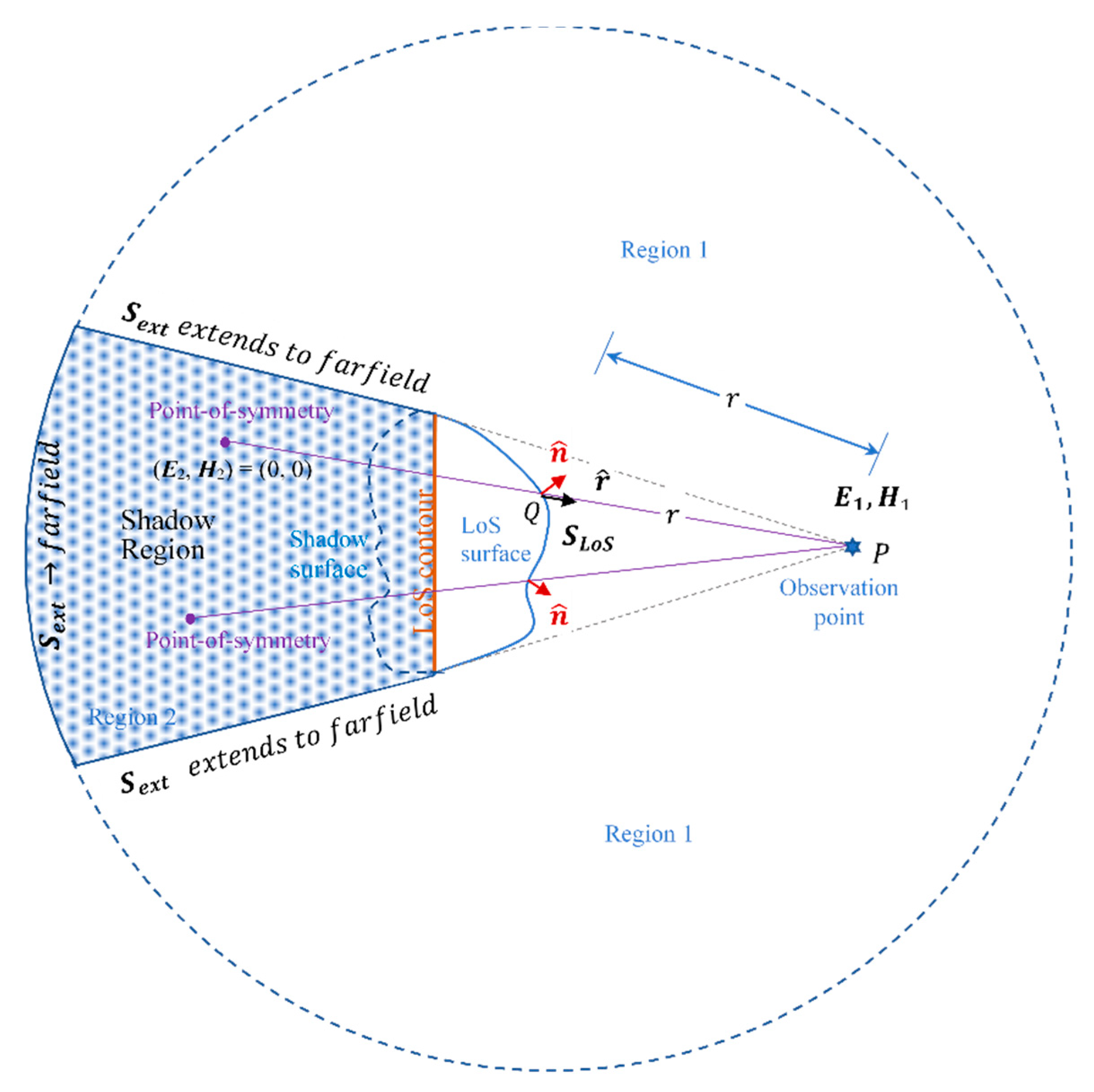
When radiation/scattering problems are solved with numerical techniques, the equivalence principle is practically the only means of far-field pattern computation. The LoS approximation, which reduces the computational time significantly in comparison with the standard equivalence approach, was introduced in [8]. It considers the source contributions from surface currents that are on the LoS surface only; as well as the currents along the LoS contour (see Figure 1). The “shadow” surface $S_{ext}$, which is not in LoS and is extended to the far-field region is suspended by the LoS contour $C_{LoS}$. The integration of the equivalent currents on $S_{ext}$ is approximated by a contour integration over the contour currents on $C_{LoS}$. The effect of the contour current is shown to be significant [8].

Here, we justify the use of only one type of surface current on the LoS surface. This improves the efficiency of the radiation pattern computations by a factor of two when used with numerical techniques such as the finite-difference time-domain (FDTD) method. This is because one radiation integral is computed instead of two.

First, we briefly review the LoS approximation to the equivalence principle; then, we present our new theory, which justifies the use of only one type of surface current on the LoS surface. In Section 4, we present an example of the computation of the radiation pattern of a microstrip patch antenna using the FDTD method. We show the comparison between the standard equivalence principle using both surface currents on the entire virtual surface and our LoS equivalence approximation with either type of surface currents that are only on the LoS surface.

2. The LoS Approximation to the Equivalence Principle

The relationship between the far zone electric field E and the electric and magnetic field vectors ${\mathit{E}}^S$ and ${\mathit{H}}^S$ on the surface enclosing the radiating sources is [5]:

$$\mathit{E}\left(P\right)\approx -\frac{j\omega {\mu }_0}{4\pi }{{\displaystyle \iint }}_S\left(\widehat{\mathit{n}}\times {\mathit{H}}^S\right)\frac{e^{-jkr}}{r}ds-\frac{j\omega \eta {\epsilon }_0}{4\pi }{{\displaystyle \iint }}_S\left[\widehat{\mathit{r}}\times \left(\widehat{\mathit{n}}\times {\mathit{E}}^S\right)\right]\frac{e^{-jkr}}{r}ds$$

(1)

here, $r$ is the distance from the surface source point Q to the observation point P, $\widehat{\mathit{n}}$ is the unit normal to the surface, $\widehat{\mathit{r}}$ is the unit vector from Q to P, k is the free-space wavenumber, $\omega$ is the frequency, and $\eta$ is the free space intrinsic impedance, the integration surface S contains all surface currents. The Green’s function is denoted as:

$$G\left(r\right)=\frac{e^{-jkr}}{4\pi r}$$

(2)

In the LoS approximation [8], the surface integrals in Equation (1) over $S_{ext}$ are replaced by contour integrals over $C_{LoS}$. The electric field at the observation point ${\mathit{E}}_1$ consist of two parts, $\left({\mathit{E}}_{1\_LoS}+{\mathit{E}}_{1\_ext}\right)$, and it is expressed as:

$$\begin{gathered} {\mathit{E}}_1\approx -j[\omega {\mu }_0{{\displaystyle \iint }}_{S_{LoS}}\left(\widehat{\mathit{n}}\times {\mathit{H}}^S\right)G\left(r\right)ds+k{{\displaystyle \iint }}_{S_{LoS}}\widehat{\mathit{r}}\times \left(\widehat{\mathit{n}}\times {\mathit{E}}^S\right)G\left(r\right)ds] \\ -j\left[{{\displaystyle \oint }}_{C_{LoS}}\left[\omega {\mu }_0\left(\widehat{\mathit{r}}\times \widehat{\mathit{n}}\right)H_R^S{C}_H+k\widehat{\mathit{n}}{E}_R^S{C}_E\right]G\left(r\right)dl\right] \end{gathered}$$

(3)

where $E_R^S$ and $H_R^S$ denote the components of the electric and magnetic field vectors along the unit vector $\widehat{\mathit{r}}$, respectively. The subscript 1 refers to the region outside the surface enclosing the sources. Region 2 is inside the surface; see the shadow region in Figure 1. The factors $C_E$ and $C_H$ are obtained from the directional derivatives along $\widehat{\mathit{r}}$ of the phase terms of the electric and magnetic fields, respectively, on the LoS contour [8]:

$$C_{E,H}={\left[-j\left({\left|\frac{d{\Theta }_{E,H}}{dr}\right|}_{C_{LoS}}+k\right)\right]}^{-1}$$

(4)

In an FDTD simulation, the radiating structures are enclosed in a volume (virtual) with absorbing boundaries to mitigate undesired reflection at the virtual boundary. The replacement of the surface integral over $S_{ext}$ with the contour integral along $C_{LoS}$ is an approximation. The error due to this approximation is typically low. For this, the worst error for field calculation with Mur’s first-order absorbing boundary condition is given by the empirical formula,

$$e_{LoS}\approx 15{\left(\frac{\lambda }{l_{\min }}\right)}^2\%$$

(5)

where $l_{\min }$ is the minimum distance between the actual radiating structure to the virtual (LoS) surface. The error contribution to the overall radiation pattern is further reduced when it is combined with the dominating component, the LoS surface currents.

The computational effort of the LoS-based pattern calculation is mostly due to the evaluation of the surface integrals over the LoS surface $S_{LoS}$. Below, we show that with the proposed LoS equivalence, only one of the two surface currents integral is required.

3. Surface Sources with LoS Equivalence

3.1. Vector Potentials and Surface Sources

The proposed theory is similar to Love’s equivalence principle [5], where the field (${\mathit{E}}_2$, ${\mathit{H}}_2$) within the enclosed region 2 is set equal to zero. Then, the equivalent surface current densities are:

$${\mathit{J}}_s=\widehat{\mathit{n}}\times {\mathit{H}}^S$$

(6)

and

$${\mathit{M}}_s=-\widehat{\mathit{n}}\times {\mathit{E}}^S$$

(7)

where ${\mathit{E}}^S$ and ${\mathit{H}}^S$ are the field vectors on the surface, and $\widehat{\mathit{n}}$ is the surface unit normal. The surface currents radiate in an unbounded medium (region 1), while the fields in region 2 are zero. The surface unit normal $\widehat{\mathit{n}}$ points toward region 1.

We represent the equivalent problem in terms of the vector potentials $\mathit{A}$ and $\mathit{F}$ due to the surface currents ${\mathit{J}}_s$ and ${\mathit{M}}_s$, respectively. In open space,

$$\mathit{A}={\mu }_0{{\displaystyle \iint }}_S{\mathit{J}}_{s}G\left(r\right)ds={{\displaystyle \iint }}_S{\mathit{A}}^{e}ds$$

(8)

and

$$\mathit{F}={\epsilon }_0{{\displaystyle \iint }}_S{\mathit{M}}_{s}G\left(r\right)ds={{\displaystyle \iint }}_S{\mathit{F}}^{e}ds$$

(9)

where ${\mathit{A}}^e={\mu }_{0}G\left(r\right){\mathit{J}}_s$ and ${\mathit{F}}^e={\epsilon }_{0}G\left(r\right){\mathit{M}}_s$ are the elemental vector potentials due to the respective current densities of the surface element. The field vectors in terms of the vector potentials are [5]:

$$\mathit{E}={\mathit{E}}_F+{\mathit{E}}_A=-\frac{1}{{\epsilon }_0}\nabla \times \mathit{F}+\frac{1}{j\omega {\mu }_0{\epsilon }_0}\nabla \times \nabla \times \mathit{A}$$

(10)

and

$$\mathit{H}={\mathit{H}}_A+{\mathit{H}}_F=\frac{1}{{\mu }_0}\nabla \times \mathit{A}+\frac{1}{j\omega {\mu }_0{\epsilon }_0}\nabla \times \nabla \times \mathit{F}$$

(11)

Ishimaru [9] refers to these relations as the Franz formulas. It can be shown [10] that the Franz formulas are equivalent to the well-known Stratton-Chu formulas,

$$\mathit{E}={{\displaystyle \iint }}_S\left[-j\omega {\mu }_{0}G\left(\widehat{\mathit{n}}\times {\mathit{H}}^S\right)-\left(\widehat{\mathit{n}}\times {\mathit{E}}^S\right)\times \nabla G-\left(\widehat{\mathit{n}}·{\mathit{E}}^S\right)\nabla G\right]ds$$

(12)

and

$$\mathit{H}={{\displaystyle \iint }}_S\left[j\omega {\mu }_{0}G\left(\widehat{\mathit{n}}\times {\mathit{E}}^S\right)-\left(\widehat{\mathit{n}}\times {\mathit{H}}^S\right)\times \nabla G-\left(\widehat{\mathit{n}}·{\mathit{H}}^S\right)\nabla G\right]ds$$

(13)

here, the gradient of G is taken with respect to the observation point. Notice that the surface integrals in Equation (3) are an approximation of the Stratton-Chu formula (12) for the case of a far-zone field.

In terms of the elemental vector potential ${\mathit{F}}^e$, ${\mathit{E}}_F$ becomes

$${\mathit{E}}_F=-\frac{1}{{\epsilon }_0}\nabla \times {{\displaystyle \iint }}_S{\mathit{F}}^{e}ds$$

(14)

as per Equation (10). Since $\nabla \times$ operates on the coordinates at the point of observation while the surface integral is over the location of the sources, these two operators can be interchanged:

$${\mathit{E}}_F=-\frac{1}{{\epsilon }_0}{{\displaystyle \iint }}_S\left(\nabla \times {\mathit{F}}^e\right)ds$$

(15)

Similarly, we obtain

$${\mathit{E}}_A=\frac{1}{j\omega {\mu }_0{\epsilon }_0}{{\displaystyle \iint }}_S\left(\nabla \times \nabla \times {\mathit{A}}^e\right)ds$$

(16)

The total field in terms of the elemental vector potentials is thus given by

$$\mathit{E}={{\displaystyle \iint }}_S\left(-\frac{1}{{\epsilon }_0}\nabla \times {\mathit{F}}^e+\frac{1}{j\omega {\mu }_0{\epsilon }_0}\nabla \times \nabla \times {\mathit{A}}^e\right) ds$$

(17)

and

$$\mathit{H}={{\displaystyle \iint }}_S\left(\frac{1}{{\mu }_0}\nabla \times {\mathit{A}}^e+\frac{1}{j\omega {\mu }_0{\epsilon }_0}\nabla \times \nabla \times {\mathit{F}}^e\right) ds$$

(18)

3.2. Field Extinction in Region 2

As per Love’s equivalence principle [5], in region 2, the condition ${\mathit{E}}_2=\mathbf{0}$ and ${\mathit{H}}_2=\mathbf{0}$ is imposed, from which the surface currents are obtained. In general, both types of currents exist on the enclosed surface. In terms of the elemental vector potentials, the condition of zero fields inside region 2 is obtained by setting the following conditions:

$$\nabla \times {\mathit{F}}_2^e=\frac{1}{j\omega {\mu }_0}\nabla \times \nabla \times {\mathit{A}}_2^e$$

(19)

and

$$\nabla \times {\mathit{A}}_2^e=-\frac{1}{j\omega {\epsilon }_0}\nabla \times \nabla \times {\mathit{F}}_2^e$$

(20)

which ensure the fulfilment of Equations (17) and (18) regardless of the shape of the enclosed surface. Here, ${\mathit{A}}_2^e$ and ${\mathit{F}}_2^e$ are elemental vector potentials of the surface currents observed in region 2.

3.3. The Observation Point and Its Point-of-Symmetry

The point-of-symmetry is a point that is radially opposite to the observation point, with the source point being at the centre of symmetry (see Figure 1). When the observation point is in the far zone, the point-of-symmetry also falls in the far zone. Thus, in the conventional equivalence principle, both the observation point and its point-of-symmetry belong to region 1 (outside the closed surface S). In the LoS equivalence, however, the point-of-symmetry belongs to the shadow region since the virtual surface S has been extended to a large (beyond far-field) conical frustum, as shown in Figure 1.

We consider the LoS surface to be regular if for each observation point and its corresponding every surface element on LoS there exists one point-of-symmetry in the shadow region. Two such points are shown in Figure 1. As an example, Figure 1 shows a conical (or pyramidal) frustum, or for a tubular frustum, the surface formed by ($S_{LoS}+S_{ext}$) would be considered regular, also the normal vector on the LoS surface would be pointing into region 1. The surface $S_{ext}$, which is not in LoS, can be approximated to a line integral, which is discussed in detail in the [8].

At the point-of-symmetry, the field of an elemental surface source has a unique relation to its counterpart at the observation point. Consider a current element in free space together with its observation point and point-of-symmetry as defined above. If the location of the observation point with respect to the source point in spherical coordinates is defined by $\left(r_1, {\theta }_1, {\phi }_1\right)$, then the location of the point-of-symmetry is

$$r_2=r_1,\hspace{1em} {\theta }_2=\pi -{\theta }_1,\hspace{1em} {\phi }_2={\phi }_1+\pi$$

(21)

Resulting in relations such as; $sin{\theta }_2=sin{\theta }_1$, $sin{\phi }_2=-sin{\phi }_1$, $cos{\theta }_2=-cos{\theta }_1$, $cos{\phi }_2=-cos{\phi }_1$. From these, the following relations are derived for the curl and the curl of the curl of the vector potential at the point-of-symmetry and the observation point:

$$\nabla \times \mathit{A}\left(r_1,{\theta }_1,{\phi }_1\right)=-\nabla \times \mathit{A}\left(r_2,{\theta }_2,{\phi }_2\right)$$

(22)

and

$$\nabla \times \nabla \times \mathit{A}\left(r_1,{\theta }_1,{\phi }_1\right)=\nabla \times \nabla \times \mathit{A}\left(r_2,{\theta }_2,{\phi }_2\right)$$

(23)

By applying the relationships defined by Equations (22) and (23) to Equations (19) and (20), we obtain the relationships between the elemental vector potentials at the point-of-symmetry $\left(r_2, {\theta }_2, {\phi }_2\right)$ and at the respective observation point $\left(r_1, {\theta }_1, {\phi }_1\right)$:

$$\nabla \times {\mathit{F}}_1^e\left(r_1, {\theta }_1, {\phi }_1\right)=-\nabla \times {\mathit{F}}_2^e\left(r_2, {\theta }_{ 2}, {\phi }_2\right)$$

(24)

$$\nabla \times \nabla \times {\mathit{F}}_1^e\left(r_1, {\theta }_1, {\phi }_1\right)=\nabla \times \nabla \times {\mathit{F}}_2^e\left(r_2, {\theta }_2, {\phi }_2\right)$$

(25)

and

$$\nabla \times {\mathit{A}}_1^e\left(r_1, {\theta }_1, {\phi }_1\right)=-\nabla \times {\mathit{A}}_2^e\left(r_2, {\theta }_2, {\phi }_2\right)$$

(26)

$$\nabla \times \nabla \times {\mathit{A}}_1^e\left(r_1, {\theta }_1, {\phi }_1\right)=\nabla \times \nabla \times {\mathit{A}}_2^e\left(r_2, {\theta }_2, {\phi }_2\right)$$

(27)

The result can be summarized as follows: (1) the curl of an elemental vector potential at the observation point is of the same magnitude but opposite sign as compared to its curl at the point-of-symmetry; (2) the curl of the curl of an elemental vector potential is the same at the observation point and its point-of-symmetry.

3.4. The Field at the Observation Point in the Far Zone

Applying the field-extinction formulas, Equations (19), (24) and (27), we obtain

$$\nabla \times {\mathit{F}}_1^e=-\frac{1}{j\omega {\mu }_0}\nabla \times \nabla \times {\mathit{A}}_1^e$$

(28)

Similarly, using Equations (20), (25) and (26), we obtain

$$\nabla \times {\mathit{A}}_1^e=\frac{1}{j\omega {\epsilon }_0}\nabla \times \nabla \times {\mathit{F}}_1^e$$

(29)

According to the Franz formulas, Equations (17) and (18), it then follows that the field at the observation point is due to the superposition of two identical terms—one due to electrical surface sources and another due to magnetic surface sources. Thus, using Equations (17) and (28), the expression for the electric field in region 1 is obtained as

$${\mathit{E}}_1=-\frac{2}{{\epsilon }_0}{{\displaystyle \iint }}_{S_{LoS}+S_{ext}}\nabla \times {\mathit{F}}_1^e ds$$

(30)

whereas the expression for the magnetic field is obtained from Equations (18) and (29) as

$${\mathit{H}}_1=-\frac{2}{{\mu }_0}{{\displaystyle \iint }}_{S_{LoS}+S_{ext}}\nabla \times {\mathit{A}}_1^e ds$$

(31)

Using the same set of equations, the fields can also be expressed as:

$${\mathit{H}}_1=\frac{2}{j\omega {\mu }_0{\epsilon }_0}{{\displaystyle \iint }}_{S_{LoS}+S_{ext}}\nabla \times \nabla \times {\mathit{F}}_1^e ds$$

(32)

$${\mathit{E}}_1=\frac{2}{j\omega {\mu }_0{\epsilon }_0}{{\displaystyle \iint }}_{S_{LoS}+S_{ext}}\nabla \times \nabla \times {\mathit{A}}_1^e ds$$

(33)

In order to translate this result into a Stratton-Chu formulation in terms of the surface field, as in Equations (12) and (13), we make use of Kirchhoff’s far-field approximation to the free-space Green’s function:

$$\tilde{G}\left(r\right)=\frac{e^{-jk\left(r+\widehat{r}\cdot r^{\prime }\right)}}{4\pi r}$$

(34)

here, $\mathit{r}=r\widehat{\mathit{r}}$ is the position vector of the observation point. It is independent of the integration point. ${\mathit{r}}^{\prime }$ is the position vector of the source (integration) point. The use of Equation (34) simplifies the differential operations on the elemental vector potentials: $\nabla$ is equal to $-jk\widehat{\mathit{r}}$, $\nabla \times$ is equivalent to $-jk\widehat{\mathit{r}}\times$ and $\nabla \times \nabla \times$ simplifies to $-k^2\widehat{\mathit{r}}\times \widehat{\mathit{r}}\times$ [8]. Using these with Equations (30) or (33) gives

$${\mathit{E}}_1=-2jk{{\displaystyle \iint }}_{S_{LoS}+S_{ext}}\widehat{\mathit{r}}\times \left(\widehat{\mathit{n}}\times {\mathit{E}}^S\right)\tilde{G}\left(r\right)ds$$

(35)

or

$${\mathit{E}}_1=-2j\omega {\mu }_0{{\displaystyle \iint }}_{S_{LoS}+S_{ext}}\left(\widehat{\mathit{n}}\times {\mathit{H}}^S\right)\tilde{G}\left(r\right)ds$$

(36)

respectively.

In the LoS, we replace the surface integrals over $S_{ext}$ with their respective contour integrals, as per Equation (3). Thus, if we compute ${\mathit{E}}_1$ through the equivalent electric surface currents, then the contribution of the LoS surface, ${\mathit{E}}_{1_{LoS}}$, becomes

$${\mathit{E}}_{1_{LoS}}=-2j\omega {\mu }_0{{\displaystyle \iint }}_{S_{LoS}}\left(\widehat{\mathit{n}}\times {\mathit{H}}^S\right)\tilde{G}\left(r\right)ds$$

(37)

and the contribution from $S_{ext}$ is approximated as

$${\mathit{E}}_{1_{ext}}\approx -2j\omega {\mu }_0{{\displaystyle \oint }}_{C_{LoS}}\left[\left(\widehat{\mathit{r}}\times \widehat{\mathit{n}}\right)H_R^S{C}_H\right]\tilde{G}\left(r\right)dl$$

(38)

The alternative computation using equivalent magnetic surface currents is also possible.

4. Discussion

The above derivations are summarized here. Equations (17) and (18) describe the field at a point in space in terms of the elemental vector potentials. The field at any point in region 1 is the integral (or sum in numerical simulation scenario) of the contributions of all elemental surface currents on the surface enclosing region 1. Furthermore, with an appropriate shape choice for the extended surface, there exists a point-of-symmetry in region 2 for every elemental surface current. If the field in region 2 were to be zero, then even for an elemental surface current contribution, the field should be zero in region 2. For each observation point in region 1, there are points-of-symmetry in region 2, corresponding to the surface currents. The fields at all these points-of-symmetry are zero, with these conditions, Equations (30) through (33) are valid.

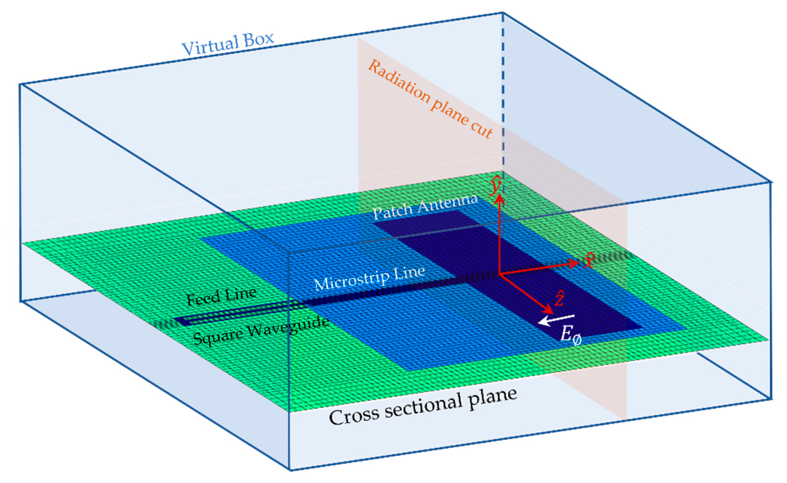
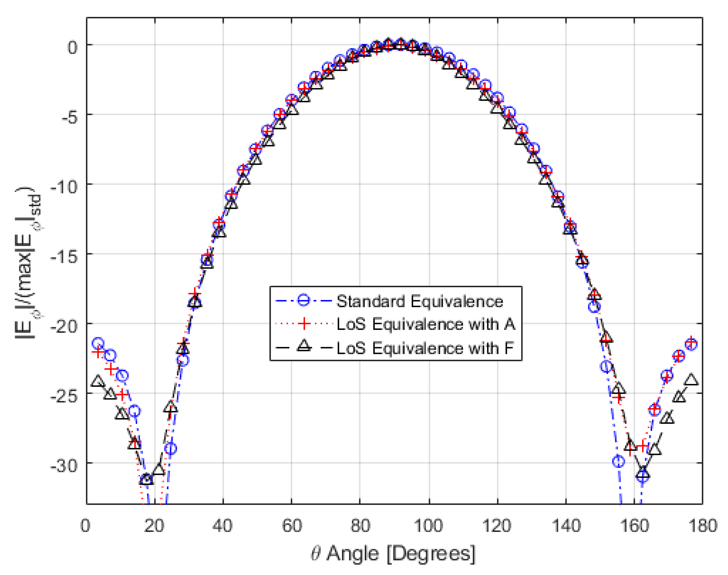
The resonant frequency of this patch antenna was determined to be 2.42 GHz. The radiation pattern is for the $E_{\varnothing }$ component and it is on the plane cut (shown in Figure 2) that is perpendicular to the antenna plane and the feed line. Figure 3 shows the simulation results for the radiation patterns for the three cases: (1) using standard equivalence with both types of surface current over the entire enclosed virtual surface; (2) using LoS approximation with only magnetic surface current and LoS-contour current; and (3) using LoS approximation with only electric surface current and LoS-contour current. All three radiation patterns were normalized to the maximum value of the standard equivalence. In general, good agreement between all three cases is observed. The minor discrepancies seen in Figure 3 near the edge are due to the approximation of the edge current integrals. This type of error was expected, and they were addressed in detail in [8].

The general LoS approximation of the far-zone field is given by Equations (3) and (4), this is also detailed in [8]. According to the theory presented above, we need to resolve either the surface integral over the equivalent electric current ($2\widehat{\mathit{n}}\times {\mathit{H}}^S$) or the one over the magnetic current ($2\widehat{\mathit{n}}\times {\mathit{E}}^S$). This improves the efficiency of the far-field radiation pattern calculations.

We apply the LoS approach with a single surface-current source type to a practical problem simulated with the FDTD method. We compute the far-field radiation pattern of a printed microstrip antenna, shown in Figure 2, and verify it by comparing with a computation based on the standard equivalence where the integration is performed over both surface current types of the whole enclosed surface. The size of the patch antenna used in the simulation is 44 × 80 mm². The substrate is of area 110 × 115 mm², the height is 1.8 mm, and the relative dielectric constant is 2.0. The feed structure of the antenna is a 50-Ω square coaxial transmission line of length 55 mm followed by a microstrip line of length 32 mm. The inner conductor of the coaxial line is of cross-sectional dimension 1.8 × 1.8 mm², the outer conductor is 5.1 × 5.1 mm², and the relative dielectric constant is 1.0.

In the FDTD simulation, the excitation source is a Gaussian pulse of width 30 ps. The total number of iterations is 1600 with 1 ps time-step interval. The mesh size used for the simulation is 120 × 70 × 120 grid cells. The size of the computation domain is 300 × 170 × 260 mm³, and the size of the virtual box (the equivalent surface) is 250 × 100 × 210 mm³. The absorbing boundaries use Mur’s first-order absorbing boundary condition [11].

5. Conclusions

We proposed an improvement to the LoS approach to the computation of antenna far-field radiation patterns using the equivalence principle. We demonstrated that, under the condition of the point-of-symmetry falling into the zero-field region, the use of one type of surface current in the LoS method does not degrade the accuracy of the computations. The validation is made with an application to a practical problem of calculating the radiation pattern of a printed patch antenna. There is remarkably good agreement between the simulation results of the improved LoS approach and the standard equivalence method. The efficiency of the new LoS approach, as compared to the standard equivalence principle, in the calculation of radiation patterns is due to the reduced computation of surface integration. The total computational time for the new LoS approach is approximately one-sixth of that required by the standard equivalence for the computation of radiation pattern in the principal plane. One half of this improvement is due to using only one type of surface current. Thus, the LoS approach is an efficient alternative to existing standard algorithms for the computation of far-field patterns in high-frequency structure simulators.

References

- Huygens, C. Treatise on Light; University of Chicago Press: Chicago, IL, USA, 1912. [Google Scholar]
- Schelkunoff, S.A. Some equivalence theorems of electromagnetics and their application to radiation problems. Bell System Tech. J. 1936, 15, 92–112. [Google Scholar] [CrossRef]
- Stratton, J.A. Electromagnetic Theory; McGraw Hill: New York, NY, USA, 1941; pp. 196–197, 482–488. [Google Scholar]
- Harrington, R.F. Time-Harmonic Electromagnetic Fields; McGraw Hill: New York, NY, USA, 1961; pp. 77–79, 101–103, 106–109, 120–123, 129–134. [Google Scholar]
- Balanis, C.A. Advanced Engineering Electromagnetics; John Wiley & Sons: New York, NY, USA, 1989; pp. 279–291, 329–342. [Google Scholar]
- Harrington, R.F. On scattering by large conducting bodies. IRE Trans. Antennas Propag. 1959, 7, 150–153. [Google Scholar] [CrossRef]
- Beckmann, P. The Depolarisation of Electromagnetic Waves; The Golem Press: Boulder, Colombia, 1968; pp. 76–92. [Google Scholar]
- Sangary, N.; Nikolova, N.K. Line-of-sight approximation to the equivalence principle for far-field computations. IEEE Trans. Antennas Propag. 2004, 52, 1890–1897. [Google Scholar] [CrossRef]
- Ishimaru, A. Electromagnetic Wave Propagation, Radiation, and Scattering; Prentice-Hall: Englewood Cliffs, NJ, USA, 1991; pp. 174–176. [Google Scholar]
- Tai, C.T. Dyadic Green’s Functions in Electromagnetic Theory; Intext Educational Publishers: New York, NY, USA, 1971. [Google Scholar]
- Mur, G. Absorbing boundary conditions for the finite-difference approximation of the time-domain electromagnetic field equations. IEEE Trans. Electromagn Compat. 1981, 23, 377–382. [Google Scholar] [CrossRef]
Figure 1.
Illustration of the line-of-sight (LoS) equivalent surface, the LoS surface contour, the shadow region, the point-of-symmetry, and the observation point.
Figure 2.
The microstrip patch antenna.
Figure 3.
The E-plane co-polarization radiation pattern of the patch antenna.
© 2020 by the authors. Licensee MDPI, Basel, Switzerland. This article is an open access article distributed under the terms and conditions of the Creative Commons Attribution (CC BY) license (http://creativecommons.org/licenses/by/4.0/).
Share and Cite
MDPI and ACS Style
Sangary, N.; Nikolova, N. Reduction of the Line-of-Sight Equivalence Principle. Electronics 2020, 9, 1278. https://doi.org/10.3390/electronics9081278
AMA Style
Sangary N, Nikolova N. Reduction of the Line-of-Sight Equivalence Principle. Electronics. 2020; 9(8):1278. https://doi.org/10.3390/electronics9081278
Chicago/Turabian StyleSangary, Nagula, and Natalia Nikolova. 2020. "Reduction of the Line-of-Sight Equivalence Principle" Electronics 9, no. 8: 1278. https://doi.org/10.3390/electronics9081278
Note that from the first issue of 2016, this journal uses article numbers instead of page numbers. See further details here.