Investigation on Unsteady Flow Characteristics in an Axial-Flow Fan under Stall Conditions

1
Research Center of Fluid Machinery Engineering and Technology, Jiangsu University, Zhenjiang 212013, China
2
Public Security College, Nanjing Forest Police College, Nanjing 210023, China
*
Author to whom correspondence should be addressed.
Processes 2020, 8(8), 958; https://doi.org/10.3390/pr8080958
Submission received: 13 June 2020
/
Revised: 29 July 2020
/
Accepted: 5 August 2020
/
Published: 9 August 2020
(This article belongs to the Section Process Control and Monitoring)
Abstract
:Based on Shear Stress Transport (SST) turbulence model for unsteady simulation of an axial-flow fan, this paper studies the time-frequency information in the hump region, and investigates the disturbance information of spike and modal wave under different flow coefficients based on continuous wavelet transform (CWT). The results show that before the hump point, the low-frequency modal wave occupies the main disturbance form and circularly propagates at 1/10 of the rotor speed, and the axial-flow fan does not enter the stall stage; while after the flow coefficient reduces to the hump point, the spike wave with higher frequency replaces the modal wave as the main disturbance mode while the axial-flow fan enters the stall stage. Through in-depth investigation of unsteady flow characteristics under the hump point, it is found that after experiencing the emerging spike, with the sharp increase of incidence angle, some flow distortions appear on the intake surface, and further induce some flow paths to form stall vortices. When a path goes into stall stage, the airflow state is greatly affected, the inverse flow and air separation phenomenon in the rim region increase significantly, and the flow capacity decreases significantly, so the flow capacity in the hub region increases correspondingly. The flow path distortion of tip leakage flow (TLF) and leading edge (LE) spillage caused by the stall vortices are the main inducements of rotating stall.
1. Introduction
As a typical rotating machine, axial-flow fan is widely used in the field of national economy due to its advantages of large air volume, good ventilation effect, high efficiency and energy savings [1,2,3]. With the development of high speed and high power in the field of rotating machinery, the axial flow fan needs to meet the design indexes of high efficiency, low noise and stable operation under multiple working conditions. However, when the axial-flow fan operates under the off-design condition, the unstable flow phenomena such as separation vortex, leakage vortex, tip vortex and wake vortex often appear [4,5]. The unstable flow will further induce the sharp increase of the incidence angle of partial flow path, and then form the reverse flow at the leading edge (LE) of the blade tip, and then finally evolve into the rotating stall, forming the stall vortex to block the flow path [6]. Due to the blocking effect of the stall vortex, the occurrence of rotating stall will cause great energy dissipation. Meanwhile, the fluid-induced vibration caused by stall vortex will aggravate the noise of axial flow fan and seriously threaten the service life of rotor blade [7,8]. Therefore, it is necessary to investigate the transient flow characteristics of axial flow fan under stall conditions.
As its wide applicability and strong harmfulness, a large number of scholars have carried out detailed research on rotating stall. Emmons first proposed the rotating stall model in 1955, and pointed out that the air flow separation in part of the flow path induced by the sharp increase of the incidence angle is the root inducement of rotating stall [9]. Then Moore, based on the nonlinear third-order partial differential equations and Galerkin procedure, showed the instantaneous characteristic changes during the transient stall process [10]. Based on the Morlet wavelet transform, Salunkhe [11] deeply explored the propagation mechanism of stall evolution under stall-inception point of the axial-flow compressor. Based on the first-order vanishing moment derivative of Gauss wavelet, Zhang [12] successfully detected the stable stall cell of the compressor in the stall-inception point.
Based on the time-frequency analysis method, the unstable disturbance characteristics under the off-design condition are revealed. There exist two different modes of disturbance, the modal disturbance belonging to long length-scale disturbance (LLSD) and spike disturbance belonging to short length-scale disturbance (SLSD) [13]. Spike disturbance is a kind of sudden precursor disturbance with high amplitude, fast circumferential propagation speed and small disturbance coverage. It belongs to the early form of the stall cell [14]. However, modal disturbance belongs to the harmonic disturbance, which has small amplitude, extremely slow circumferential propagation speed and great disturbance coverage. It is not a stall disturbance mode, but only an unstable flow field disturbance of rotating machinery under off-design conditions [15]. Camp [16] summarizes the relationship between spike and modal disturbance forms, external characteristic curve and critical incidence angle. The results show that when the incidence angle of the hump point does not reach the critical incidence angle value, the disturbance mode belongs to the modal disturbance; while the rotor incidence angle before the hump point or at the hump point is higher than the stall critical incidence angle, then the spike disturbance mode appears.
In this paper, SST k-ω turbulence model is used to simulate the unsteady flow characteristics of an axial-flow fan under stall conditions. The pressure fluctuation characteristics of the axial-flow fan under various stall conditions are studied. The frequency of each stage under the spike-stall mode is analyzed in detail based on CWT, and the unsteady flow behaviors of the hump point are analyzed. The transition process from weak disturbances to unstable strong disturbances under spike-stall mode is investigated.
2. Numerical Aspects and Computational Details
2.1. Simulation Model and Grid Generation
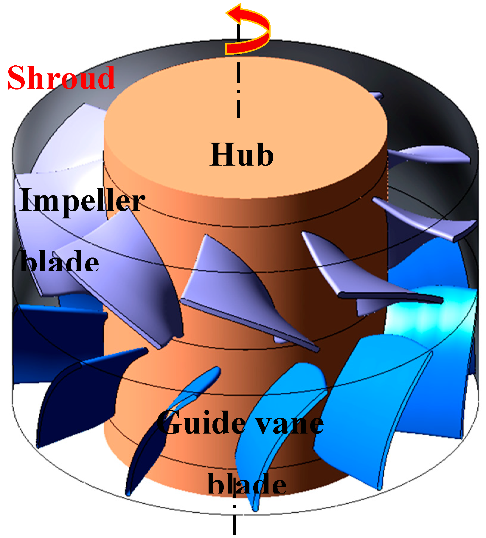
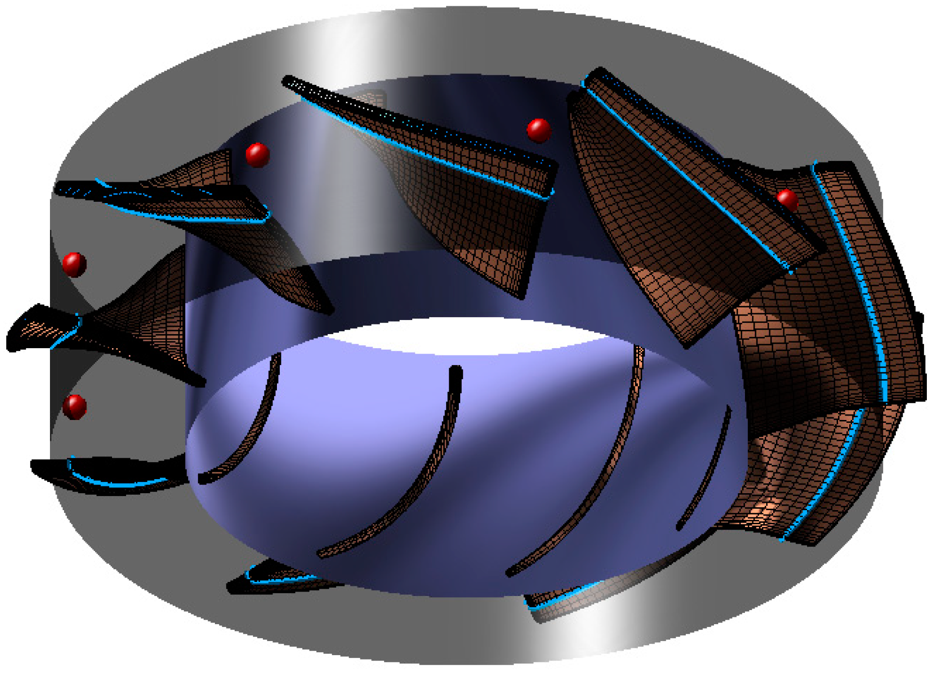
Figure 1 shows the 3D model of the axial-flow fan; the whole simulation model consists of inlet pipe, impeller, guide vane and outlet pipe.
In order to avoid the reverse flow from inlet and outlet and ensure the uniformity of inlet and outlet flow, the inlet and outlet pipe were extended to a certain size. The length of the straight pipe of inlet and outlet is set as 5 × D2, while D2 is the diameter of the rotor. In the process of numerical simulation, the model of axial-flow fan is simplified, the installation base and outlet grille are omitted, and the motor region is replaced by cylinder, which improves the quality of grid and reduces the workload of numerical simulation while not affecting the accuracy. The parameters of axial-flow fan are listed in Table 1.
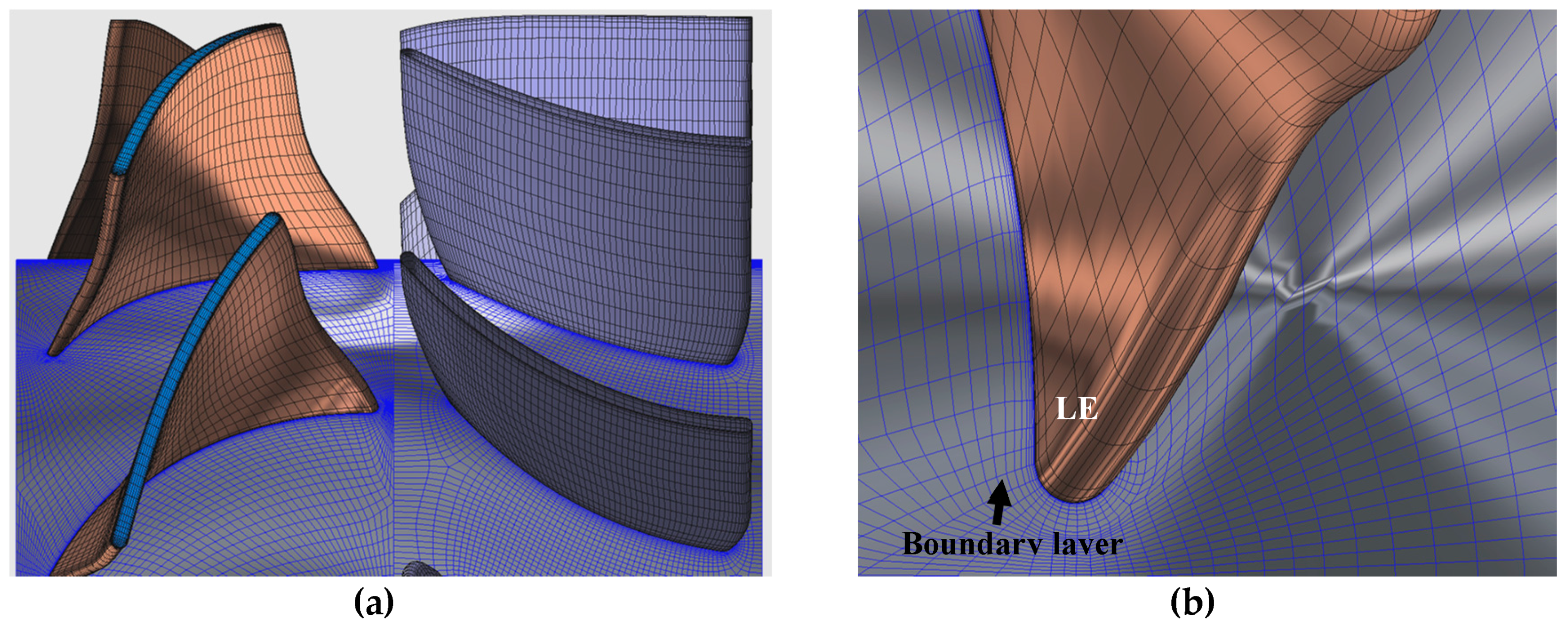
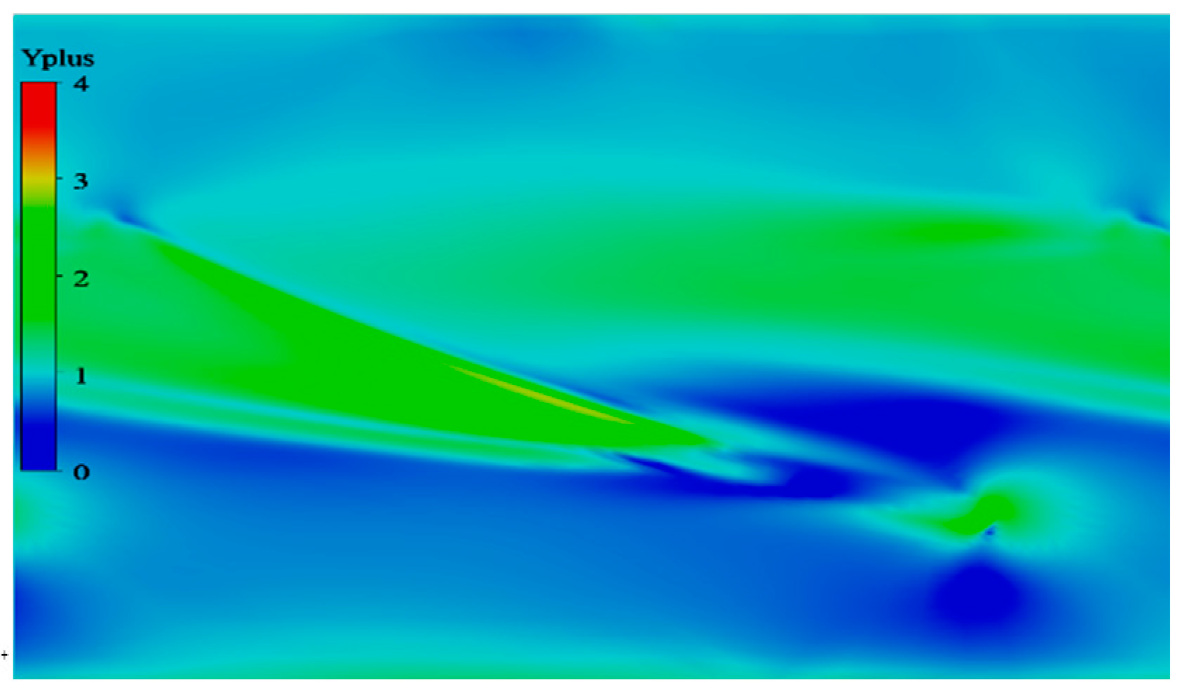
As the mesh quality has a direct relationship with the accuracy of the numerical results, Turbo-Grid software is used as the refined mesh generation of impeller and guide vane, which is shown in Figure 2. By arranging 10 nodes in the boundary layer and controlling the thickness of the first layer to 0.005 mm, the automatic near-wall treatment was employed to suit the requirements of SST k-ω turbulence model. As shown in Figure 3, the y+ of blade tip is controlled within 5. Under the rated condition, the average y+ value of blade tip region is 1.63, the maximum value is 4.65, and the minimum value is 0.45, which meets the y+ requirements of the turbulence model.
2.2. Mesh Independence Verification
By using the same numerical simulation settings and mesh topology, Table 2 shows the mesh independence verification only by changing the number of mesh nodes and size. As can be seen from Table 2, the pressure rise coefficient ψ changes little with the increase of mesh number, and the error is less than 1%, meeting the mesh independence verification requirements. In addition, by adjusting the number of mesh nodes and the height of the first layer mesh, the average y+ value of the wall decreases with the increase of the mesh number. Based on the above factors, Mesh scheme C is selected as the computational grid.
2.3. Turbulence Model and Boundary Conditions
The assembled simulation field is imported into ANSYS-CFX for numerical simulation. According to the operation characteristics of the axial-flow fan, the setting of boundary conditions is determined. The transport medium is an ideal incompressible airflow, and SST k-ω turbulence model is used. The boundary conditions of import and export are set as free inflow and mass outflow, respectively. The no-slip boundary condition is adopted for the wall surface. Each computing domain is connected by the interface. The inlet and outlet pipes, as well as the stator are all set as static regions, and the rotor is set as rotating region with a speed of 6000 r/min. The convergence at each physical time step was achieved in 4 to 10 iterations when the root mean square residual dropped below 10−5.
3. Applicability of Turbulence Model and Experimental Verification
According to the GB/T 1236-2000 standard, the axial flow fan test bench for aerodynamic performance test was set up; the test device diagram is shown in Figure 4. The experimental system includes an axial-flow test fan, centrifugal auxiliary fan, rectifying grid plate, static pressure measuring hole, throttle orifice plate, auxiliary joint, round damper regulator and test air duct. The performance test system is a MGS fan performance test system. The MGS test system includes a frequency conversion controller, motor power tester, photoelectric speed probe, tachometer, sound level meter, static pressure transmitter, ambient atmospheric pressure temperature and humidity sensor, industrial computer, acquisition host and other instruments and equipment. Figure 5 shows the physical model of the rotor.
The fan performance is commonly presented in terms of the static-to-static pressure rise coefficient ψ:
Versus flow coefficient φ:
where: pin—is the inlet pressure, pout—is the outlet pressure, ρ—is the air density, u—is the rotor peripheral velocity, D—is the rotor diameter, and Q—is the fan flow rate.
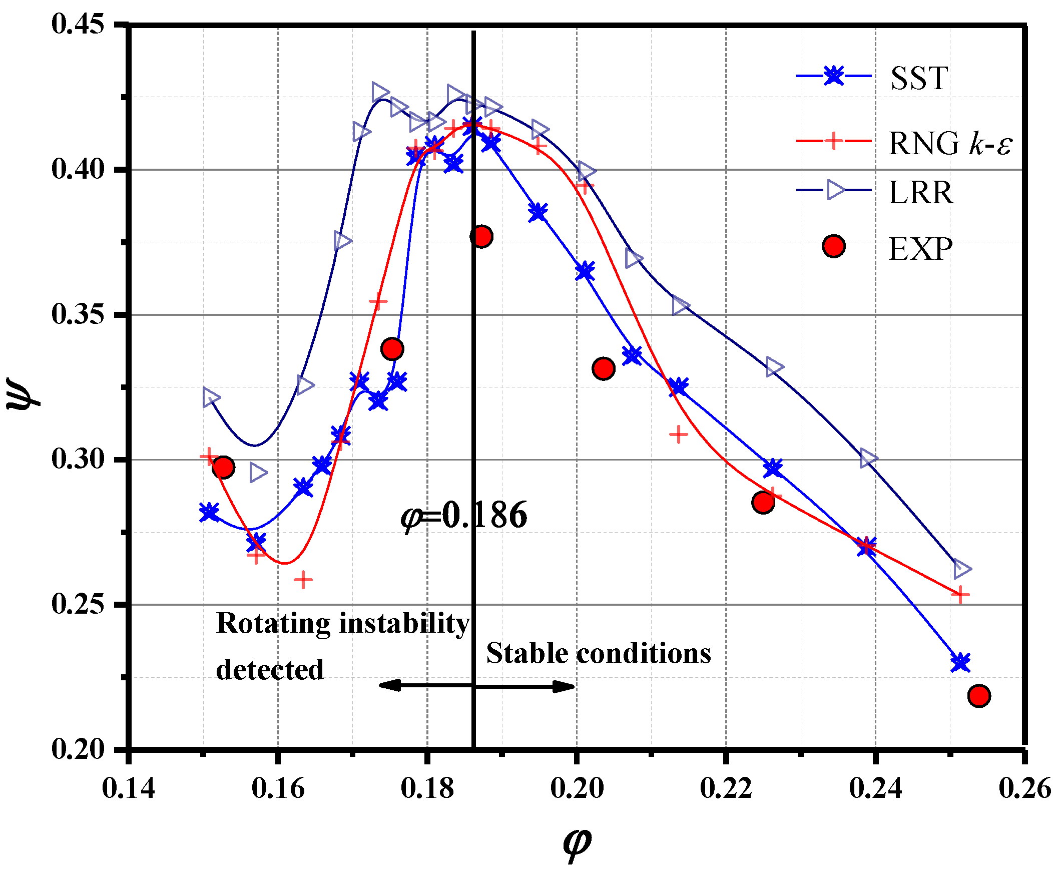
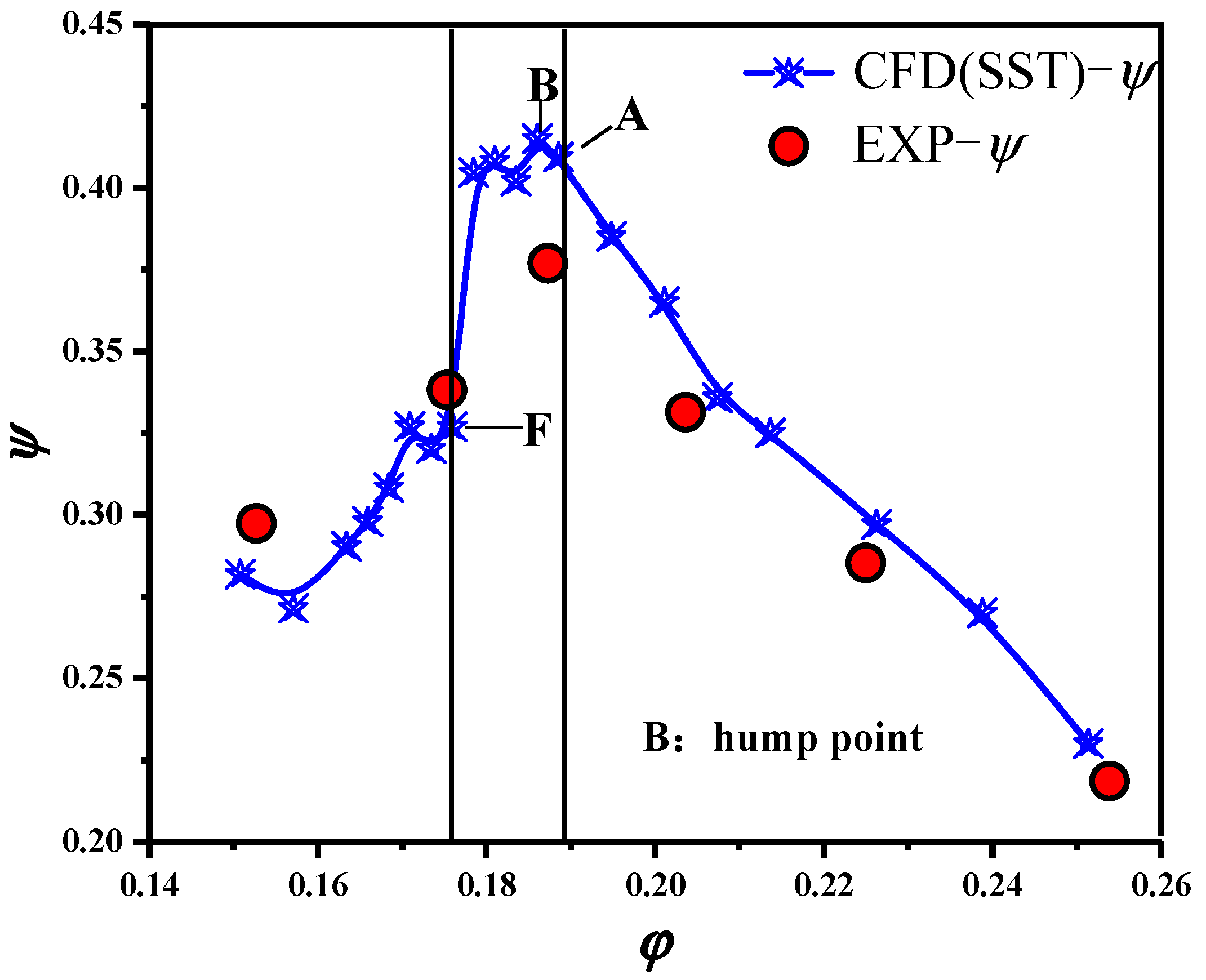
In the case of keeping the grid division and boundary conditions consistent, the SST turbulence model, RNG k-ε turbulence model and LRR turbulence model are respectively used for the numerical simulation of axial-flow fan. The aerodynamic characteristic curve is obtained through comparative simulation, and the selection of turbulence model is verified, as shown in Figure 6. The highest point of pressure rise coefficient ψ in hump region is defined as the “hump point”.
The performance curves of the axial-flow fan obtained by the three turbulence models all have the same waveform, and all turbulence models calculate the similar hump region. For the prediction of the initial operating point of rotating instability, the three turbulence models all get the same results, the versus flow coefficient at hump point is φ = 0.186. Compared with the experimental aerodynamic performance data, the prediction results of SST model and RNG k-ε turbulence model are generally better than LRR model, and the aerodynamic performance curve of LRR turbulence model is significantly higher than that of the other two turbulence models and the experimental data. Compared with SST model and RNG k-ε model, the predicted static pressure rise coefficient of RNG k-ε model has a large deviation from the experimental value under the point of large flow rate (φ = 0.186), which is worse than that of SST turbulence model. In addition, the predicted results of the SST turbulence model match well with the experimental values, and the deviation from the experimental data is the best, whether in the large flow rates (stable condition) or in the small flow rates. However, there is a deviation between the CFD and EXP value at the hump point, and the deviation is 7.9%—less than 10%. In conclusion, SST turbulence model has a good match for the performance prediction of the axial-flow fan, and can correctly predict the performance and flow characteristics.
Figure 7 shows the typical operation line simulated by SST turbulence model. When operating at the hump point or the left side of the hump point, the fan will probably step into the rotating stall. During this process, based on the unsteady numerical simulation, there is a pressure fluctuation of the fan under the stall conditions near the hump point (Figure 7A–F).
4. Results and Discussion
4.1. Pressure Fluctuation Characteristics of Axial-Flow Fan under Stall Conditions
The pressure coefficient Cp is used for dimensionless treatment of dynamic pressure to express the intensity of pressure fluctuation. The equation is as follows:
where p is the dynamic pressure of the monitoring points; is the average pressure in the rotation period of the monitoring points; and u2 is the peripheral speed of the impeller outlet; 1 t* represents the time required for impeller to rotate one revolution in the circumferential direction.
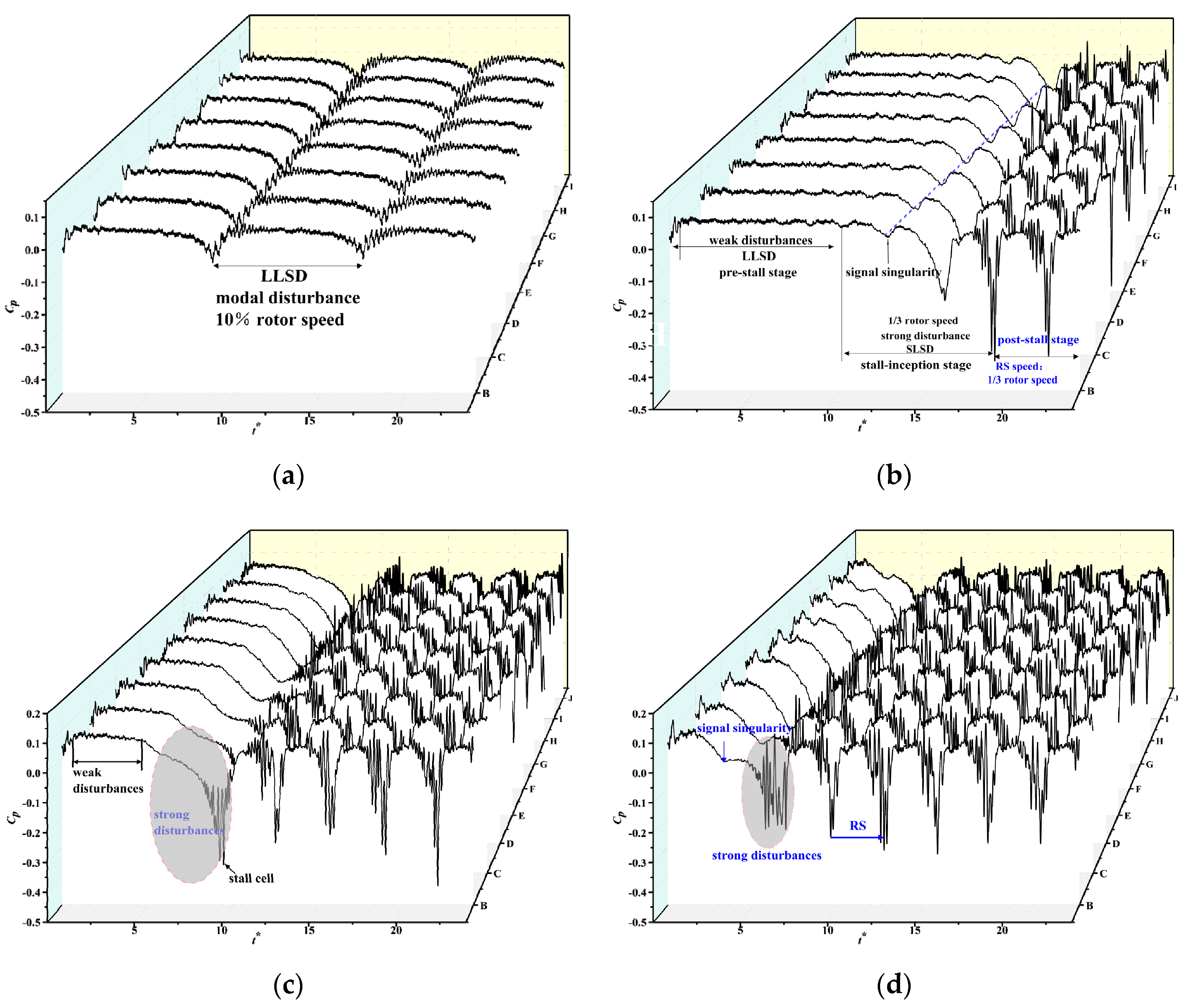
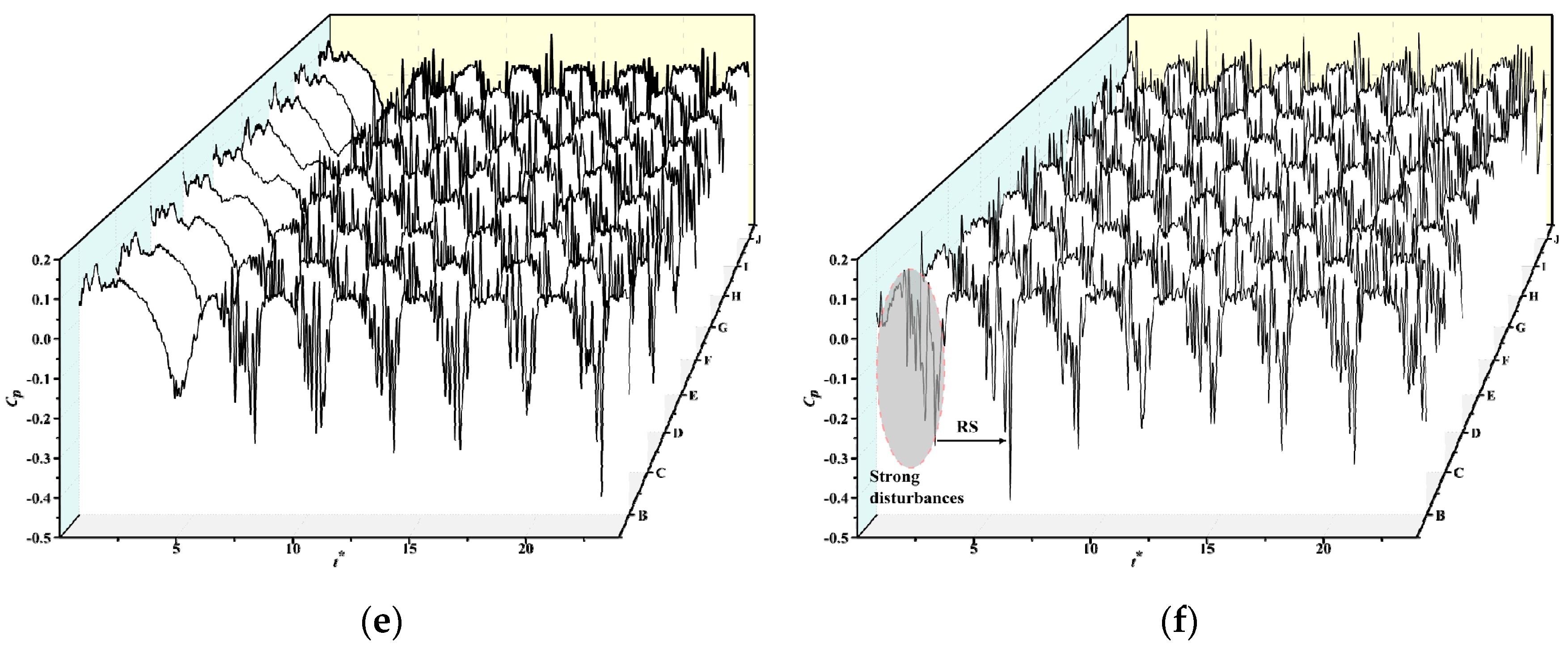
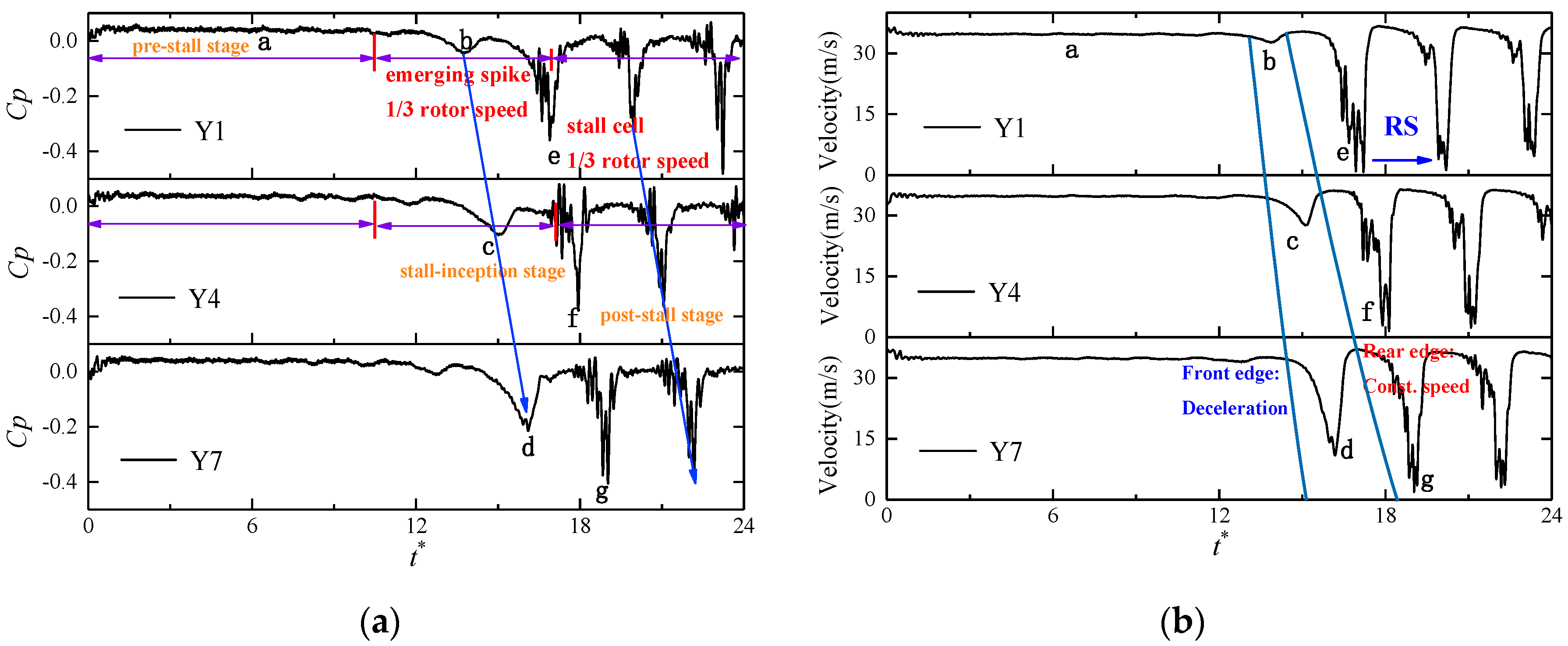
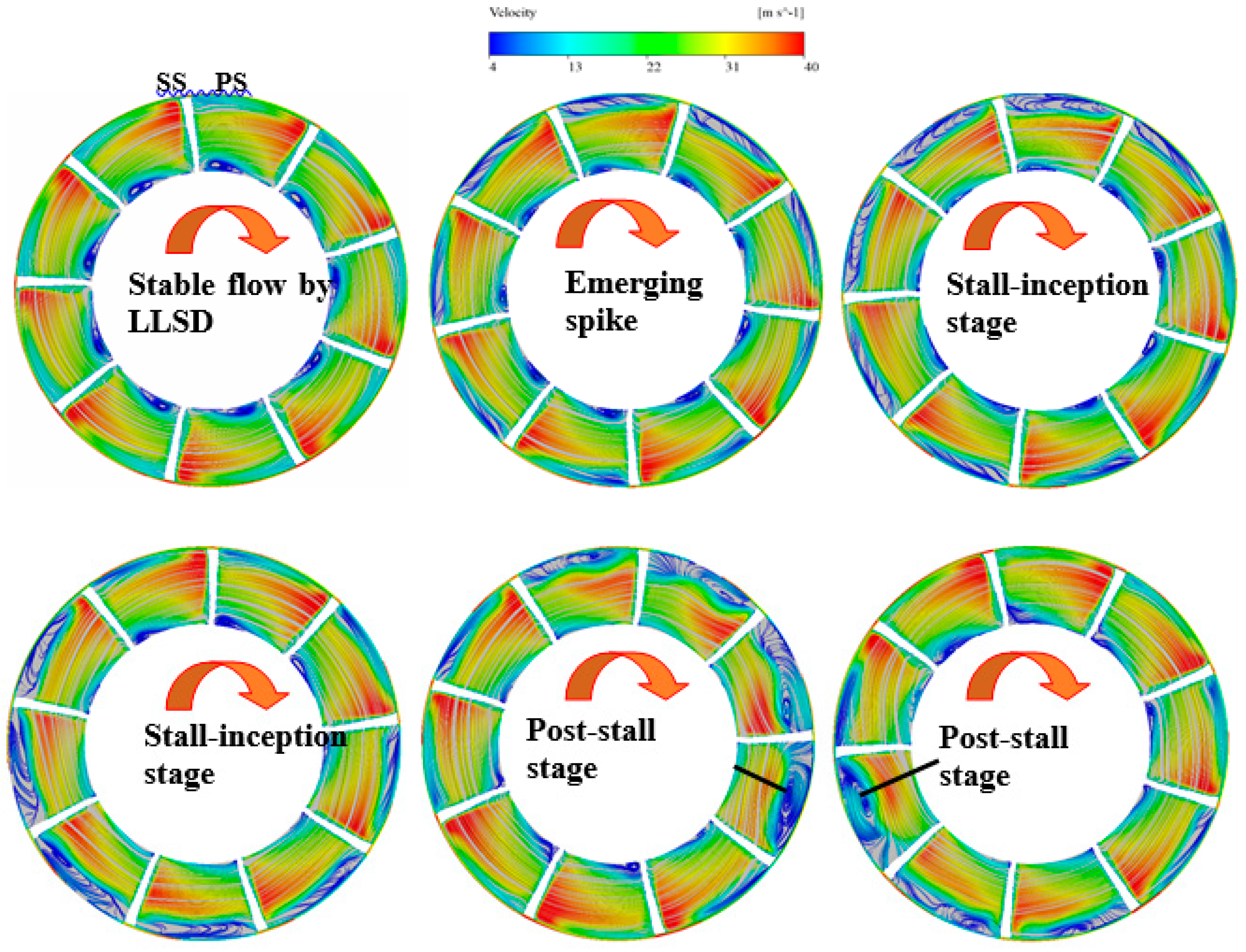
Figure 8 shows the location of monitoring points, and Figure 9 shows the pressure fluctuation characteristics of axial flow fan under different flow coefficients. In order to clearly show the rotating stall characteristics, the working conditions near the hump point are selected for research. As the main influence region of rotating stall is the rim region, so the monitoring points are located in the middle section of rotor, and located at 0.8 span. The definition of each stage under the stall conditions is as follows. The term “stall-inception” will be used to describe the time period during which a rotating disturbance grows into a fully developed stall cell and the term “pre-stall” will be used to describe the time period prior to stall-inception; the term “post-stall” will be used to describe the time period which the axial-flow fan is fully controlled by rotating stall (RS).
The pressure fluctuation curves of operation point A (OP-A) in different flow channels are consistent, showing large-scale and low-amplitude transient characteristics. Meanwhile, OP-A is located on the right side of the hump point. Due to the above reasons, the axial-flow fan is only disturbed by the modal wave under this flow coefficient, with a period of 8.75 t*, so the circumferential propagation speed of modal disturbance is about 1/10 of the rotor speed. Compared with OP-A, the pressure fluctuation characteristics of the hump point (OP-B) have changed greatly. After experiencing a 10 t* weak disturbance of LLSD, the axial flow fan will show the signal singularity. The strong disturbance from the spike wave will gradually replace the modal wave as the main disturbance form. With the impeller rotating, the strong disturbance effect will gradually increase, and it will evolve into a circumferential propagation of the stable stall cell. The period of SLSD and rotating stall is the same, and their circumferential propagating speed is about 1/3 rotor speed. With the further reduction of the flow coefficient (OP-C–OP-E), the emerging time of signal singularity (spike) will gradually advance, the control time of fan system disturbed by modal wave will further reduce, and each path will step into the stall state in advance, while the propagating speed of SLSD and stall cell will remain unchanged. Under the point of OP-G, the fan system will be subject to strong disturbance from rotating stall at the initial time, and the modal disturbance will disappear basically.
As rotating stall is a transient evolution process from signal singularity to a developed stall cell, the traditional Fast Fourier transform (FFT) is unable to capture the time and frequency information of the signal at the same time, and continuous wavelet transform (CWT) has been proven useful in uncovering mechanisms of spike or modal type stall.
In this paper, the Morlet wavelet, which is representative of nonorthogonal wavelet bases, is used in continuous wavelet transform. The Morlet wavelet is the real part and imaginary part of the amplitude are harmonic vibration signals; Meanwhile, as a nonorthogonal wavelet, the Morlet wavelet as the wavelet base for CWT. In addition, its scale changes continuously, and can adjust the time and frequency domain resolution as required.
The mathematical equation of Morlet wavelet ψ(t) is as follows:
In Equation (4), t represents time, fb represents wavelet bandwidth, and fc represents center frequency.
In practical application, complex wavelet can easily lead to phase distortion. Therefore, the real part of Morlet wavelet is often used as wavelet function, and the mathematical equation is as follows:
Its Fourier transform ϕ(t) can be expressed as follows:
In this paper, the sine function signal is used to verify the applicability of continuous wavelet transform. The equation is shown as follows
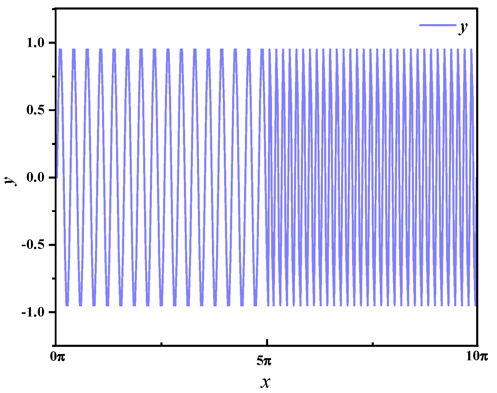
At different times, the equation of the sine function signal is y = sin(2πx) and y = sin(4πx), the frequency of the two signal is 1 Hz and 2 Hz partly, and the sampling frequency of the signal is 10 Hz. The time domain generated is also shown in Figure 10. After adjusting the appropriate center frequency and frequency bandwidth, the spectrum distribution obtained by Morlet wavelet is shown in Figure 11. The frequency spectrum shows that when 0 < x < 5π, the main frequency of the signal is 1 Hz; when 5π < x < 10π, the main frequency of the signal is 2 Hz. Hence, the accuracy of CWT can be verified.
For the pressure fluctuation signal of axial-flow fan under different working conditions, it belongs to one-dimensional signal, the general form of one-dimensional CWT is shown in Equation (8).
where x(t) is the time domain information, and ψ(t) is the wavelet function. The symbol ψ* represents complex conjugate. s is the scaling parameter, and b is the translation parameter.
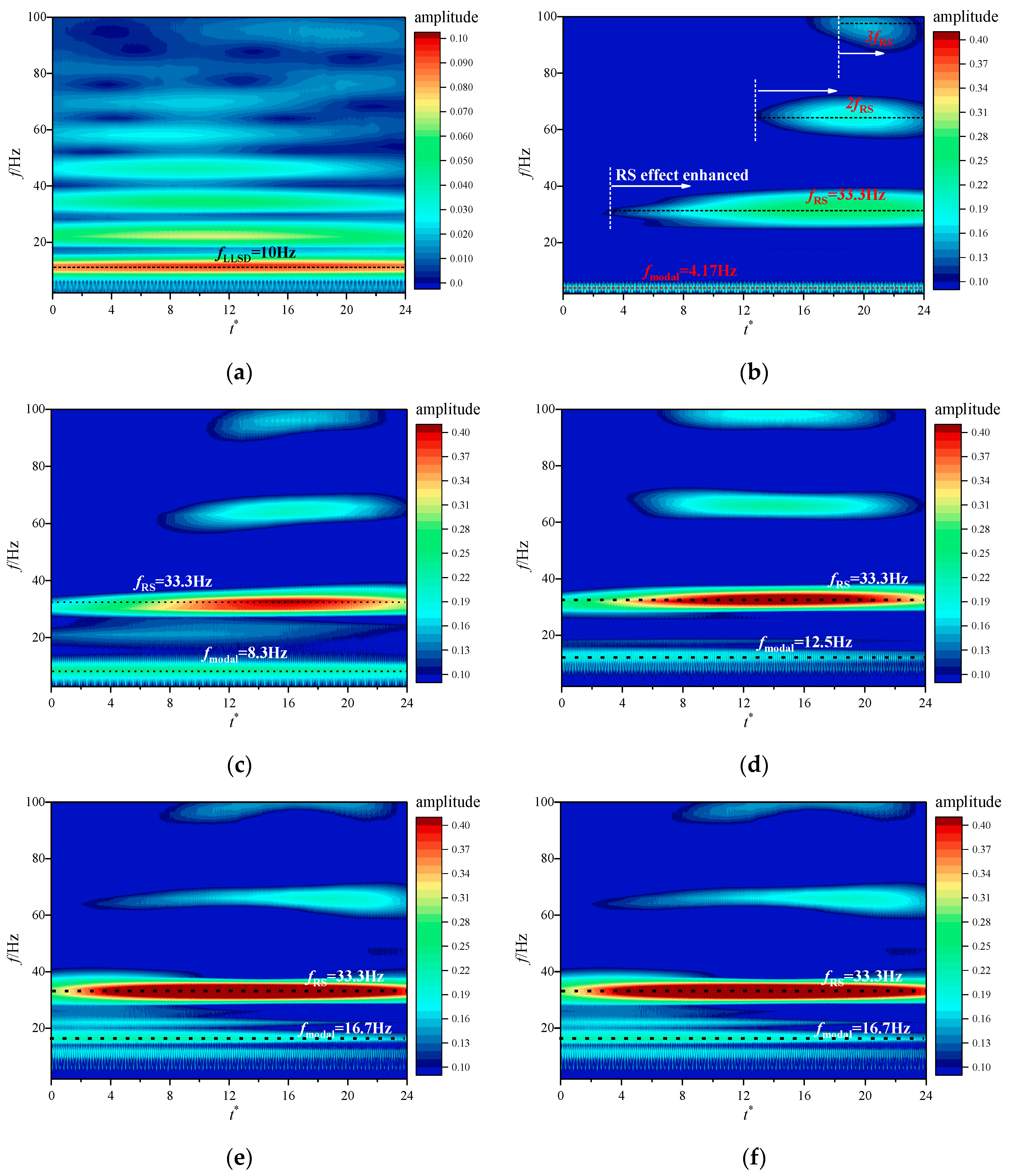
Based on CWT, Figure 12 shows the time-frequency distribution characteristics of dynamic pressure signals at different flow rates, and discusses the differences of time-frequency distribution in pre-stall stage, stall-inception stage and post-stall stage.
Before the hump point, all paths of rotor are occupied by LLSD, so the frequency band of 8–12 Hz appears in the time-frequency diagram. Among them, the maximum pressure fluctuation energy (main frequency) is appears near 10 Hz. Under OP-A condition, the monitoring points are only disturbed by LLSD and will not be affected by RS, modal disturbance is a harmonic type disturbance formed before the formation of stall cell, so the frequency and amplitude of LLSD remain unchanged. The amplitude caused by modal disturbance is relatively low, and the circumferential propagation speed is very slow.
At the hump point, the rotor will experience pre-stall, stall-inception and post-stall stage successively. Different from the pre-stall stage, the flow path is only disturbed by the low amplitude and long period disturbance mode from modal wave. In the stall-inception stage, after experiencing spike emerging, the stall cell with higher amplitude and faster circumferential rotation speed gradually form in the flow path. Although the low amplitude disturbance brought by modal wave still exists, but the spike disturbance of higher amplitude replaces it and becomes the dominant frequency. Each path of impeller will not only be disturbed by LLSD, but also by rotating stall with higher amplitude and faster propagation period. As can be seen from Figure 8, the propagation speed of SLSD is the same as the propagation speed of the stall cell which is 1/3 of the rotor speed, so the visual reflection of SLSD and rotating stall disturbance in the frequency spectrum is fRS = 33.3 Hz.
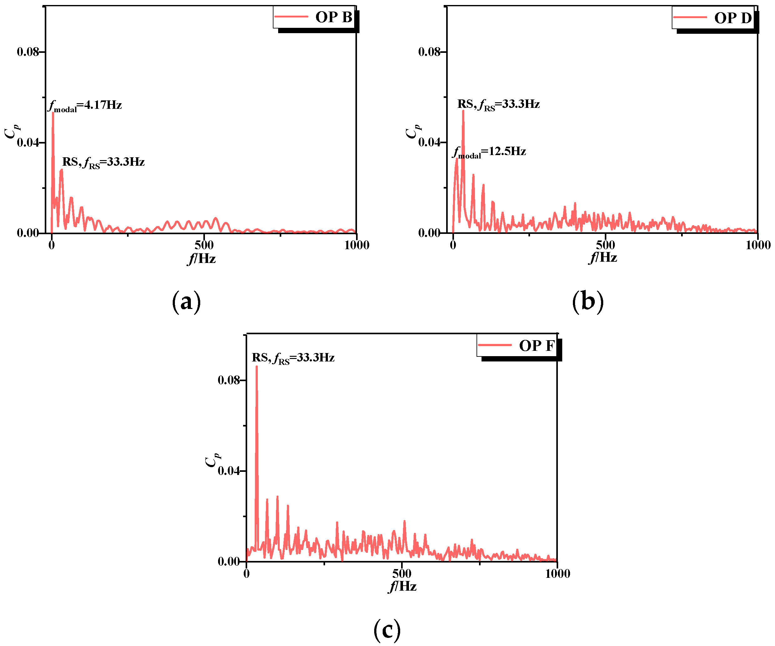
With the decrease of the flow coefficient, the difference of time-frequency distribution begins to appear, which is mainly reflected in the changes of frequency and amplitude of fLLSD and fRS. First of all, with the decrease of flow coefficient, the occurrence time of rotating stall is a little earlier, and the stall effect is gradually enhanced, but the propagation period of a single stall cell remains unchanged, so the frequency of fRS reflected in the time-frequency diagram remains unchanged, but the appearance time and amplitude of fRS increase significantly with the decrease of flow coefficient. In contrast, with the decrease of flow coefficient, the frequency band range of fLLSD increases from 4.17 Hz to 16.7 Hz. From the FFT results in Figure 13, it can be seen that with the decrease of flow coefficient, the pressure fluctuation energy caused by LLSD gradually decreases, so the amplitude of fLLSD also decreases. While in the deep stall point (OP-F), the pulsation induced by the weak disruption from LLSD is reduced to the pole, and each path is always controlled by the stall cell from the initial time period, and the stall effect is always throughout the transient flow process of axial-flow fan, so fRS does not show the trend of gradually enhancing with the impeller rotation like the hump point (OP-B), its amplitude basically remains unchanged, and the induced pressure fluctuation energy is higher than OP-B.
4.2. Analysis of Transient Flow Characteristics under Hump Point
As the hump point is the initial condition of rotating stall, so it is necessary to further study the transient flow characteristics at hump point, and explore the transient distortion process generated by emerging spike. Figure 14 shows the pressure and velocity fluctuation characteristics of the hump point, and the monitoring points are Y1, Y4 and Y7 respectively. The velocity fluctuation waveform is consistent with that of static pressure. After the emerging spike, the flow velocity decays with the flow separation at LE, and finally decreases to 0 m/s. At this moment, the air flow cannot be discharged from the flow path smoothly, and the whole rim region of the stall path is seriously blocked. According to the disturbance mode and pressure fluctuation waveform of spike stall, the characteristic time a–g is selected, and the selected time is as shown in Figure 14.
The meridional velocity reflects the flow capacity of the axial-flow fan. Based on the assumption that the cylinder layer is independent, the velocity gradient equation of the axial-flow fan is taken as the basis, and the equation of the meridional velocity is as follows:
where, ω is the angular velocity, rad/s; and Γ(r) is the airfoil blade circulation. The calculation formula is as follows:
where: W∞(r) represents the relative velocity of each blade; l(r) represents the chord length of each blade.
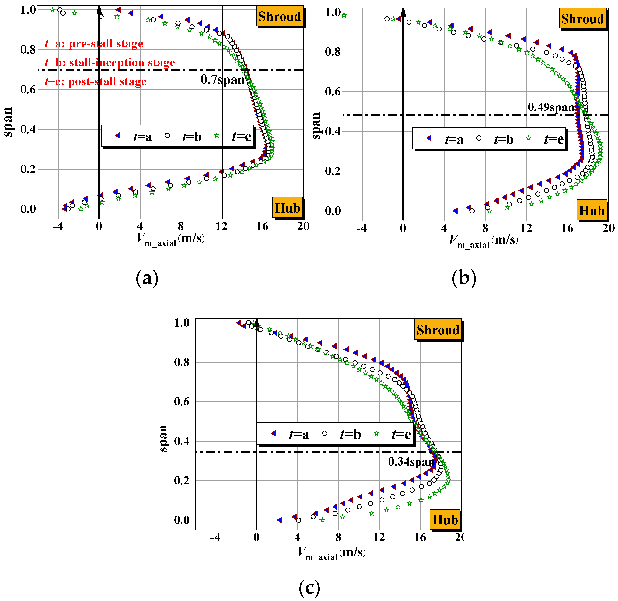
Since the meridional velocity Vm is the velocity vector, its value is always positive, and its flow direction cannot be displayed. Therefore, this paper divides the meridional velocity according to the XYZ direction, and counts the data of the axial component of the meridional velocity (Vm_aixal).
As can be seen from Figure 15, in different cross-sections of the rotor, Vm_axial keeps the trend of increasing first and then decreasing gradually from hub to rim side in each time period. Among them, the maximum value of Vm_axial is existing in 0.25–0.4 span. In this region, the axial flow fan has the strongest overcurrent capacity. However, in the rim region, the whole surface has negative values. The disturbance and countercurrent phenomenon of tip leakage flow under part-loading conditions are still the main factors that affect the flow capacity and blade construction of the axial flow fan, especially the inverse flow at LE. As the axial-flow fan changes from a weak disturbance of LLSD to a strong disturbance of SLSD and further evolves into rotating stall, the flow pattern and overcurrent capacity of the fan change greatly. After experiencing emerging spike, the velocity of the whole rim flow surface is attenuated, and the rim region disturbed by SLSD and rotating stall was blocked, so the air flow could not be smoothly discharged, and then flow into the hub region. Therefore, the axial velocity of the hub region was further increased in the stall state, and the vortex on the hub side under the stall path was also disappeared, and the flow capacity was enhanced. In the process from pre-stall stage to post-stall stage, with the increase of chord length coefficient, the position of span where meridional velocity attenuation decreases. At the intake surface, the stall disturbance effect is mainly concentrated in the rim region; while in the outlet surface, the velocity decays at 0.34 span, the stall blocking effect is the most obvious at this span.
Figure 16 shows the transient distribution characteristics of the incidence angle in the inlet surface of the rotor under the hump point. The equation of the incidence angle is as follows:
where: vaxial is the axial velocity, m/s; v is the local speed, m/s; and θ is the blade inlet setting angle, °.
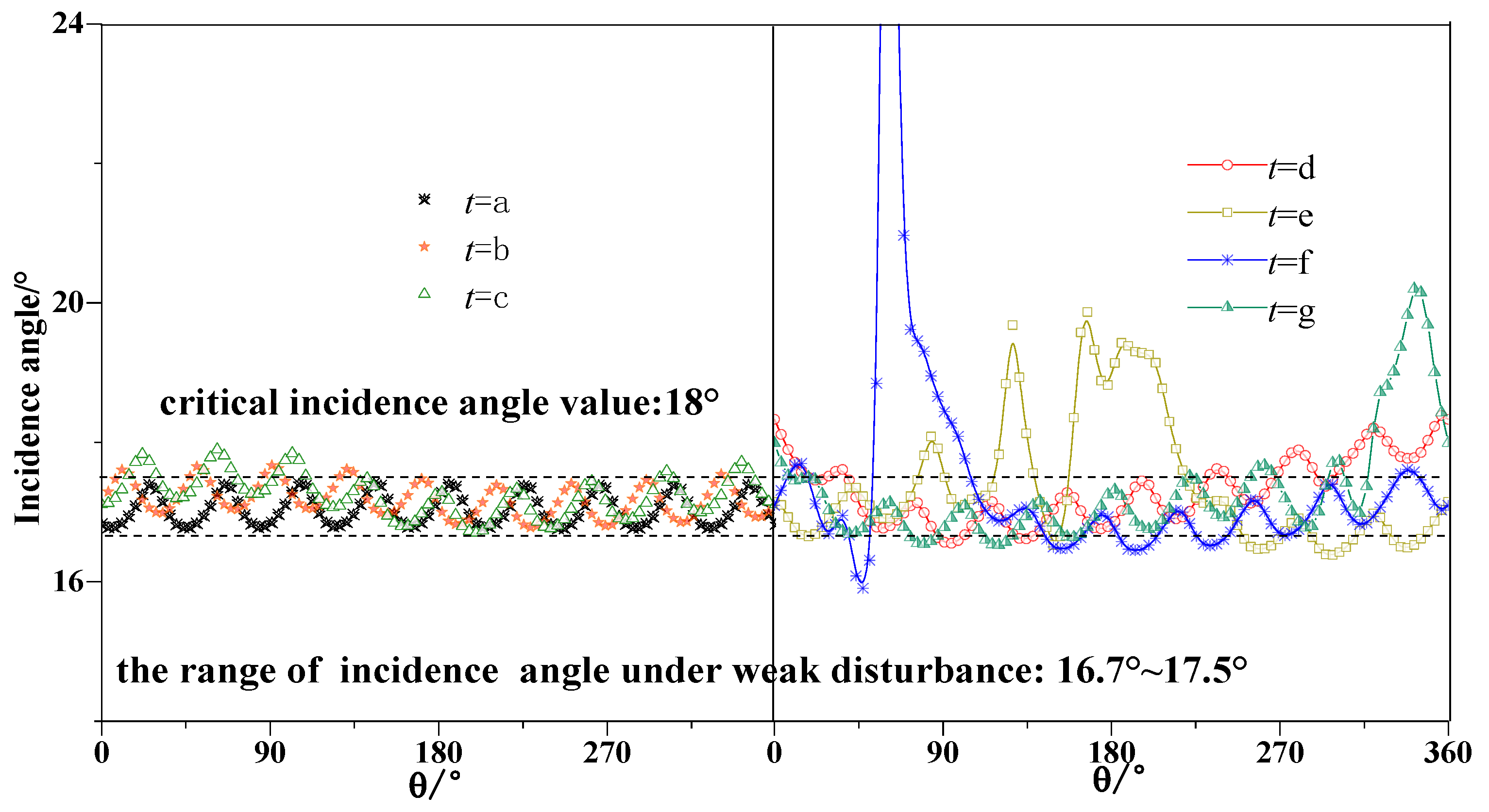
As the stall cell is located in the rim region and the distortion induced by rotating stall is the most significant in rim region, the transient distribution characteristics of incidence angle at 0.8 span are counted.
In the pre-stall stage, the axial-flow fan is not affected by rotation stall, but only by LLSD’s weak disturbance. Therefore, the distribution of incidence angle of each path is basically the same, and the incidence angle basically keeps periodic oscillation in the range of 16.7–17.5°. At this time, the incidence angle has not reached the critical value, and the internal flow characteristics of fan are relatively stable. Due to the reason of impeller rotation, there is a certain phase difference in the distribution characteristics of the incidence angle at different time. However, with the sudden appearance of spike emerging, SLSD replaces LLSD as the main disturbance, the incidence angle of one path is slightly higher than that of the earlier stage, and gradually reaches the critical value, and a small amount of flow separation phenomenon occurs in the rim region. Therefore, when t = b, the signal in one path appears a sharp shock wave, and the pressure shows a small sharp drop, so the critical value is about 18°.
As the impeller rotates, the sharp increase of the incidence angle induced by SLSD becomes worse. In the stall-inception stage (b–d), with the impeller rotating, the incidence angle of one passage is gradually increasing, and the flow separation phenomenon on the suction side is gradually intensified. However, as the stall cell is in the developing stage, the surge of the incidence angle is relatively small, and the rise range is about 1°. However, in the post-stall stage, the sharp increase of incidence angle is further intensified, which is far higher than the critical incidence angle. The inflow angle has been reduced to nearly 0°. In the stall path, a large amount of air flows close to the suction surface in LE, and a large area of boundary layer flow separation phenomenon occurs, and many vortices are formed. Meanwhile, as the propagation period of rotating stall is lower than the rotor speed, there is a certain phase difference in the range of the sharp increase of incidence angle at different times.
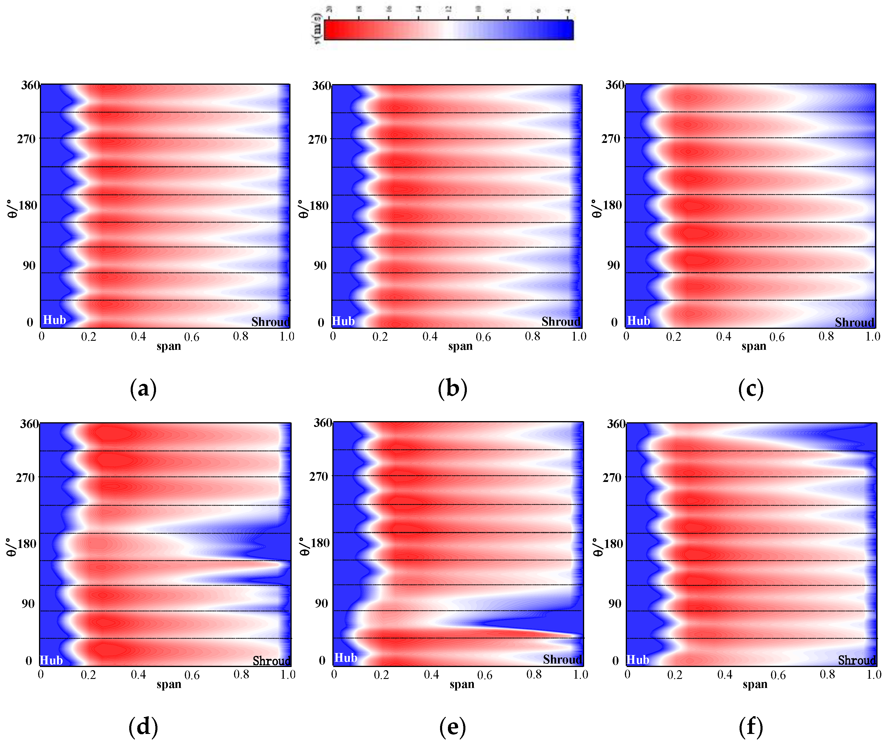
With the emergence of spike disturbance, the incidence angle increases sharply as well as the flow pattern of the inlet surface changes. Figure 17 shows the transient flow characteristics of the inlet surface at the hump point. In order to show the difference of flow distribution in each path more clearly, the space rectangular coordinate system is transformed into the cylindrical coordinate system. As shown in Figure 16, Path 1 is in the range of 0–40°, Path 2 is in the range of 40–80°, and so on.
At the moment of the emerging spike, similar to the change of incidence angle, the inflow pattern does not show obvious distortion. The distribution of the inlet flow pattern is uniform, and the flow pattern of each path is basically the same. The low-velocity flow region only appears on the hub and rim side, while the flow velocity on the hub side is relatively lower. However, with the continuous disturbance of spike, the low-velocity flow region on the rim side gradually extends to the lower span side, the flow paths gradually show the difference of inflow quality, and the inflow pattern presents a circumferential uneven distribution, such as the moment of t = d. After the spike disturbance mode is further transformed into the developed rotating stall, the difference of inflow is further intensified. At this moment, the low-velocity region near the rim side has spread to 0.5 span, and interferes with several adjacent paths. The phenomenon of distorted flow in the rim region is intensified, which directly affects the sharp deterioration of the flow pattern. In the post-stall stage, the low-velocity region of the inlet surface also propagates in the circumferential direction of the flow path, its propagation speed is the same as the stall propagation speed, and opposite to the rotation direction of the rotor.
Figure 18 shows the transient flow characteristics in the middle section of the rotor to show the evolution and development of rotating stall. In the pre-stall stage, the axial flow fan is only disturbed by modal wave, and the flow in the rim region is relatively stable without flow distortion. In the hub region, as the blade angle of the hub side is larger than the inlet flow angle, the formation of negative incidence angle causes the flow separation near the pressure surface of each path. With the emergence of spike, the inlet flow angle of the rim region gradually breaks through the critical value, and the flow distortion spreads to multiple passages, accompanied by the decrease of the air velocity and flow capacity in the rim region. In the stall-inception and post-stall stage, flow distortion in the rim region is gradually intensified, and the stall vortex is formed gradually. In the flow path disturbed by rotating stall, the flow in the rim region is distorted, and the flow is squeezed to the flow surface of the hub. Therefore, the flow angle of the hub surface gradually increases, and the flow separation phenomenon in the hub region gradually disappears. However, the flow in the rim region is relatively stable in the flow path which is not disturbed by rotating stall, and there is still a large area of separated flow in its hub side.
Figure 19 shows the transient flow characteristics of the rotor outlet surface at the hump point. Like the flow characteristics of the inlet surface and the middle section of the rotor, the flow in the rim region is gradually distorted and the low-velocity airflow region is gradually formed after experiencing the emerging spike. Then, the fully developed stall cell propagates counter-clockwise on the outlet surface, and the circumferential velocity is far lower than the rotor rotation speed.
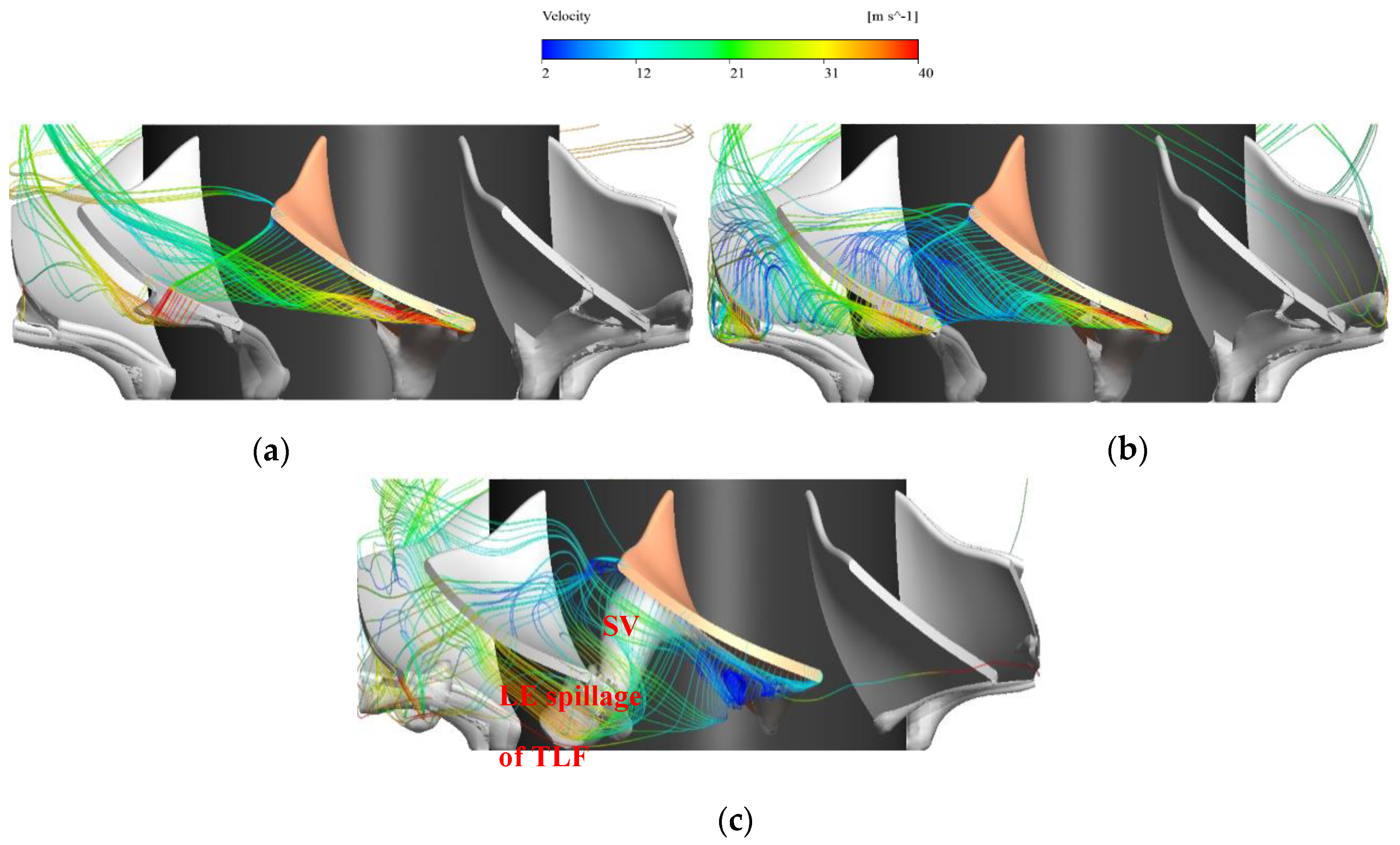
The emerging spike and rotating stall will not only affect the flow pattern of different cross-sections, but also directly change the flow pattern and trajectory of TLF. Figure 20 shows the transient process of tip leakage flow from the pre-stall stage to post-stall stage, and iso-surface is used to characterize the low-pressure flow region in the rotor to better show the stall vortex.
In the pre-stall stage, the flow pattern of TLF is relatively stable, most of TLF can flow smoothly out of the rotor from leading edge (LE) to trailing edge (TE), while a small amount of TLF from TE flows into the next path along the rotor shroud through the tip clearance, and there is no obvious distortion in the TLF. In the stall-inception stage, TLF deteriorated rapidly after expiring emerging spike. With the distortion caused by the surge of incidence angle, the leakage flow pattern changed greatly. TLF has been unable to flow out of the rotor smoothly. Due to the phenomenon of flow separation, the airflow velocity of TLF has been attenuated. A large amount of TLF flows into the next path through the tip clearance, seriously interferes with the downstream flow field, and there is a tendency of condensation to form in the vortex in the downstream path. In the post-stall stage, the trajectory of TLF changed again. Due to the blocking effect of the stall vortex, TLF is unable to smoothly discharge the flow path. Meanwhile, the phenomenon of tip overflow through the tip clearance also decreased. The trajectory of most TLF is distorted due to the blockage effect, part of TLF forms a vortex under the stall interference effect, and presents the inverse flow situation. After TLF flows back to LE, it flows close to the suction surface of the downstream blade and overflows into the downstream path, gradually changes the flow pattern of the downstream path, and triggers the surge of the incidence angle, which causes the flow separation and promotes the counter-clockwise circumferential propagation of rotating stall. The fundamental reason for the circumferential propagation of rotating stall is that the blocking effect of the stall vortex leads to the distortion of the trajectory of TLF. The distorted TLF flows into the next flow path in the form of LE spillage, and then changes the flow pattern of the downstream flow path.
5. Conclusions
- (1)
- On the right side of the hump point, the axial-flow fan will only be disturbed by modal wave; At the hump point, the spike wave will replace the modal wave as the main disturbance form; On the left side of the hump point, the spike disturbance amplitude will decay with the decrease of the flow rate, and the periodic large-scale oscillation of the signal induced by rotating stall will become the main disturbance.
- (2)
- At the hump point, after experiencing an emerging spike, the incidence angle of partial flow paths begins to distort, gradually rises, surpasses the critical value, and gradually forms the low-speed countercurrent in the rim region of the intake surface. With the rapid deterioration of the inflow quality of partial paths, the flow pattern is gradually distorted and condensed to form stall vortices and block the path. Same as the circumferential propagation mode of stall vortex, the mode of incidence angle and distortion inflow pattern will propagate circumferentially at the same propagation speed.
- (3)
- After the emerging spike, due to the effect of rotating stall disturbance, the different cross-sections of the rotor present different degrees of velocity attenuation. With the increase of chord length coefficient, the position of span where meridional velocity attenuation decreases. At the intake surface, the stall disturbance effect is mainly concentrated in the rim region, while in the outlet surface, the velocity decays at 0.34 span. After the formation of the developed stall cell, due to the large-area blockage in the rim region, the air flow is squeezed to the hub side, the flow capacity of the hub side is gradually enhanced, and the separation vortex on the hub side induced by the modal disturbance is also gradually disappeared.
- (4)
- Due to the emergence of spike and the stall cell, the flow path of TLF will change significantly. As there is an interference in the path by the developed stall cell, the flow distortion of TLF will occur due to the blockage effect, and the LE spillage will occur to interfere with the downstream path. The flow path distortion caused by rotating stall is the fundamental inducement of the circumferential propagation of stall cell.
Author Contributions
Methodology and project administration, X.Z.; writing—original draft preparation and review and editing, C.J., M.L.; review and editing, C.J., E.L. and X.Z. All authors have read and agreed to the published version of the manuscript.
Funding
This research was funded by the National Key Research and Development Program of China (No. 2016YFC0400202), the Key R&D Project of Jiangsu Province (Modern Agriculture) (No. BE2018313), and the Priority Academic Program Development of Jiangsu Higher Education Institutions (PAPD).
Conflicts of Interest
The authors declare no conflicts of interest.
Nomenclature
| Symbols | |||
| Z | Number of impeller blades | Rs | rotor shroud diameter (mm) |
| Zd | Number of guide vane blades | Rh | rotor hub diameter (mm) |
| δ | tip clearance (mm) | t* | time for rotating one revolution |
| ψ | pressure rise coefficient | α | incidence angle (°) |
| φ | versus flow coefficient | vaxial | axial velocity (m/s) |
| u | rotor peripheral velocity | Vm | meridional velocity (m/s) |
| Cp | pressure coefficient | ω | angular velocity (m/s) |
| x(t) | time series | Γ(r) | airfoil blade circulation |
| ψ(t) | wavelet function | W∞(r) | relative velocity of each blade (m/s) |
| ψ* | complex conjugate | l(r) | chord length of each blade |
| b | translation parameter | u2 | Blade outlet speed (m/s) |
| s | scaling parameter | fbpf | Blade Passing Frequency (Hz) |
| fb | wavelet bandwidth | fc | center frequency (Hz) |
| Abbreviations | |||
| LLSD | long length-scale disturbance | LE | leading edge |
| SLSD | short length-scale disturbance | TE | trailing edge |
| CFD | computational fluid dynamics | OP | operation point |
| PS | pressure surface | SS | suction surface |
| EXP | experiment | CWT | Continuous Wavelet Transform |
| RS | rotating stall | TLF | tip leakage flow |
| FFT | Fast Fourier Transform | ||
References
- Ye, X.; Ding, X.; Zhang, J.; Chunxi, L. Numerical simulation of pressure pulsation and transient flow field in an axial flow fan. Energy 2017, 129, 185–200. [Google Scholar] [CrossRef]
- Fike, M.; Bombek, G.; Hriberšek, M.; Hribernik, A. Visualisation of rotating stall in an axial flow fan. Exp. Therm. Fluid Sci. 2014, 53, 269–276. [Google Scholar] [CrossRef]
- Luo, B.; Chu, W.; Zhang, H. Tip leakage flow and aeroacoustics analysis of a low-speed axial fan. Aerosp. Sci. Technol. 2020, 98, 105700. [Google Scholar] [CrossRef]
- Park, K.; Choi, H.; Choi, S.; Sa, Y. Effect of a casing fence on the tip-leakage flow of an axial flow fan. Int. J. Heat Fluid Flow 2019, 77, 157–170. [Google Scholar] [CrossRef]
- Salunkhe, P.B.; Joseph, J.; Pradeep, A. Active feedback control of stall in an axial flow fan under dynamic inflow distortion. Exp. Therm. Fluid Sci. 2011, 35, 1135–1142. [Google Scholar] [CrossRef]
- Greitzer, E.M. Surge and Rotating Stall in Axial Flow Compressors—Part I: Theoretical Compression System Model. J. Eng. Power 1976, 98, 190–198. [Google Scholar] [CrossRef]
- Li, W.; Li, E.; Ji, L.; Zhou, L.; Shi, W.; Zhu, Y. Mechanism and propagation characteristics of rotating stall in a mixed-flow pump. Renew. Energy 2020, 153, 74–92. [Google Scholar] [CrossRef]
- Righi, M.; Pachidis, V.; Könözsy, L.; Pawsey, L. Three-dimensional through-flow modelling of axial flow compressor rotating stall and surge. Aerosp. Sci. Technol. 2018, 78, 271–279. [Google Scholar] [CrossRef]
- Emmons, H.W.; Pearson, C.E.; Grant, H.P. Compressor surge and stall propagation. Trans. ASME 1955, 127, 455–469. [Google Scholar]
- Greitzer, E.M.; Moore, F.K. A Theory of Post-Stall Transients in Axial Compression Systems: Part II—Application. J. Eng. Gas Turbines Power 1986, 108, 231–239. [Google Scholar] [CrossRef]
- Salunkhe, P.B.; Pradeep, A. Stall Inception Mechanism in an Axial Flow Fan Under Clean and Distorted Inflows. J. Fluids Eng. 2010, 132, 121102. [Google Scholar] [CrossRef]
- Zhang, H.; Yu, X.; Liu, B.; Wu, Y.; Li, Y. Using wavelets to study spike-type compressor rotating stall inception. Aerosp. Sci. Technol. 2016, 58, 467–479. [Google Scholar] [CrossRef]
- Nishioka, T.; Kuroda, S.; Kozu, T. Spike and Modal Stall Inception Patterns in a Variable-pitch Axial-flow Fan. Proc. JSME Annu. Meet. 2003, 2, 27–28. [Google Scholar] [CrossRef]
- Spakovszky, Z.S.; Roduner, C.H. Spike and Modal Stall Inception in an Advanced Turbocharger Centrifugal Compressor. J. Turbomach. 2009, 131, 031012. [Google Scholar] [CrossRef]
- Nishioka, T.; Kanno, T.; Hayami, H. G601 Effect of End-Wall Flow on Modal Stall Inception Pattern in a Variable-Pitch Axial Flow Fan. In Proceedings of the Fluids Engineering Conference, San Diego, CA, USA, 30 July–2 August 2007; p. _G601-1_. [Google Scholar]
- Camp, T.R.; Day, I.J. A Study of Spike and Modal Stall Phenomena in a Low-Speed Axial Compressor; Volume 1: Aircraft Engine; Marine; Turbomachinery; Microturbines and Small Turbomachinery; American Society of Mechanical Engineers: New York, NY, USA, 1997. [Google Scholar] [CrossRef] [Green Version]
Figure 1.
Axial-flow fan model.

Figure 2.
The computational mesh of the axial-flow fan. (a) Impeller and guide vane; (b) Local mesh refinement near blade.
Figure 2.
The computational mesh of the axial-flow fan. (a) Impeller and guide vane; (b) Local mesh refinement near blade.

Figure 3.
y+ distribution of blade tip.

Figure 4.
Experiment system for the axial-flow fan.

Figure 5.
Physical model of rotor: (a) left view, (b) front view.

Figure 6.
Performance curve simulated by different turbulence models comparing with experimental data.
Figure 6.
Performance curve simulated by different turbulence models comparing with experimental data.

Figure 7.
Performance curve of the axial flow fan.

Figure 8.
Location of monitoring points.

Figure 9.
Pressure fluctuation characteristics of axial flow fan–operating point (OP) A–F. (a) φ = 0.189 − OP-A; (b) φ = 0.186 − OP-B; (c) φ = 0.183 − OP-C; (d) φ = 0.181 − OP-D; (e) φ = 0.178 − OP-E; (f) φ = 0.176 − OP-F.
Figure 9.
Pressure fluctuation characteristics of axial flow fan–operating point (OP) A–F. (a) φ = 0.189 − OP-A; (b) φ = 0.186 − OP-B; (c) φ = 0.183 − OP-C; (d) φ = 0.181 − OP-D; (e) φ = 0.178 − OP-E; (f) φ = 0.176 − OP-F.


Figure 10.
Time frequency waveform of the signal.

Figure 11.
Spectrum based on Morlet wavelet.

Figure 12.
Spectrum chart based on CWT–OP A–F. (a) φ = 0.189 − OP-A; (b) φ = 0.186 − OP-B; (c) φ = 0.183 − OP-C; (d) φ = 0.181 − OP-D; (e) φ = 0.178 − OP-E; (f) φ = 0.176 − OP-F.
Figure 12.
Spectrum chart based on CWT–OP A–F. (a) φ = 0.189 − OP-A; (b) φ = 0.186 − OP-B; (c) φ = 0.183 − OP-C; (d) φ = 0.181 − OP-D; (e) φ = 0.178 − OP-E; (f) φ = 0.176 − OP-F.

Figure 13.
Spectrum chart based on FFT–OP B, D and F. (a) OP-B; (b) OP-D; (c) OP-F.

Figure 14.
Transient pulsation process of signal under hump point. (a) Transient pressure fluctuation process; (b) Transient velocity fluctuation process.
Figure 14.
Transient pulsation process of signal under hump point. (a) Transient pressure fluctuation process; (b) Transient velocity fluctuation process.

Figure 15.
Axial meridional velocity distribution characteristics at different cross-sections: (a) inlet surface, (b) middle surface, (c) outlet surface.
Figure 15.
Axial meridional velocity distribution characteristics at different cross-sections: (a) inlet surface, (b) middle surface, (c) outlet surface.

Figure 16.
Distribution characteristics of transient incidence angle at 0.8 span.

Figure 17.
Distribution of transient inflow characteristics at hump point: (a) t = b. (b) t = c. (c) t = d, (d) t = e, (e) t = f, (f) t = g.
Figure 17.
Distribution of transient inflow characteristics at hump point: (a) t = b. (b) t = c. (c) t = d, (d) t = e, (e) t = f, (f) t = g.

Figure 18.
Transient flow characteristics in the middle section of rotor.

Figure 19.
Transient flow characteristics of the rotor outlet surface.

Figure 20.
Transient process of tip leakage flow from pre-stall stage to post-stall stage: (a) pre-stall stage, (b) emerging spike, (c) post-stall stage.
Figure 20.
Transient process of tip leakage flow from pre-stall stage to post-stall stage: (a) pre-stall stage, (b) emerging spike, (c) post-stall stage.


Table 1.
Parameters of axial-flow fan model.
| Parameter | Value |
|---|---|
| Rotor Speed n (RPM) | 6000 |
| Number of Impeller Blades Z | 9 |
| Number of Guide Vane Blades Zd | 11 |
| Shroud Diameter Rs (mm) | 141.8 |
| Hub Diameter Rh (mm) | 86.4 |
| Tip Clearance of Impeller δ (mm) | 0.5 |
Table 2.
Mesh independence verification of the axial-flow fan.
| Mesh Scheme | Mesh Elements | First Layer Cell Height of Impeller (mm) | Mean y+ of Wall | ψ/ψA |
|---|---|---|---|---|
| A | 1.56 × 10⁶ | 0.02 | 13.24 | 1 |
| B | 2.13 × 10⁶ | 0.01 | 4.73 | 1.003 |
| C | 2.89 × 10⁶ | 0.005 | 1.65 | 0.998 |
© 2020 by the authors. Licensee MDPI, Basel, Switzerland. This article is an open access article distributed under the terms and conditions of the Creative Commons Attribution (CC BY) license (http://creativecommons.org/licenses/by/4.0/).
Share and Cite
MDPI and ACS Style
Jiang, C.; Li, M.; Li, E.; Zhu, X. Investigation on Unsteady Flow Characteristics in an Axial-Flow Fan under Stall Conditions. Processes 2020, 8, 958. https://doi.org/10.3390/pr8080958
AMA Style
Jiang C, Li M, Li E, Zhu X. Investigation on Unsteady Flow Characteristics in an Axial-Flow Fan under Stall Conditions. Processes. 2020; 8(8):958. https://doi.org/10.3390/pr8080958
Chicago/Turabian StyleJiang, Chenlong, Mengjiao Li, Enda Li, and Xingye Zhu. 2020. "Investigation on Unsteady Flow Characteristics in an Axial-Flow Fan under Stall Conditions" Processes 8, no. 8: 958. https://doi.org/10.3390/pr8080958
Note that from the first issue of 2016, this journal uses article numbers instead of page numbers. See further details here.