Stochastic Properties of Confidence Ellipsoids after Least Squares Adjustment, Derived from GUM Analysis and Monte Carlo Simulations

1
Institut of Geodesy and Photogrammetry, Technische Universität Braunschweig, Bienroder Weg 81, 38106 Braunschweig, Germany
2
Geotec Geodätische Technologien GmbH, 30880 Laatzen, Germany
*
Author to whom correspondence should be addressed.
Mathematics 2020, 8(8), 1318; https://doi.org/10.3390/math8081318
Submission received: 30 June 2020
/
Revised: 30 July 2020
/
Accepted: 3 August 2020
/
Published: 8 August 2020
(This article belongs to the Special Issue Stochastic Models for Geodesy and Geoinformation Science)
Abstract
:In this paper stochastic properties are discussed for the final results of the application of an innovative approach for uncertainty assessment for network computations, which can be characterized as two-step approach: As the first step, raw measuring data and all possible influencing factors were analyzed, applying uncertainty modeling in accordance with GUM (Guide to the Expression of Uncertainty in Measurement). As the second step, Monte Carlo (MC) simulations were set up for the complete processing chain, i.e., for simulating all input data and performing adjustment computations. The input datasets were generated by pseudo random numbers and pre-set probability distribution functions were considered for all these variables. The main extensions here are related to an analysis of the stochastic properties of the final results, which are point clouds for station coordinates. According to Cramer’s central limit theorem and Hagen’s elementary error theory, there are some justifications for why these coordinate variations follow a normal distribution. The applied statistical tests on the normal distribution confirmed this assumption. This result allows us to derive confidence ellipsoids out of these point clouds and to continue with our quality assessment and more detailed analysis of the results, similar to the procedures well-known in classical network theory. This approach and the check on normal distribution is applied to the local tie network of Metsähovi, Finland, where terrestrial geodetic observations are combined with Global Navigation Satellite System (GNSS) data.
1. Introduction
For decades, the quality concepts in geodesy have been based on classical statistical theory and generally accepted assumptions, such as the normal distribution of observations, possible correlation between observations and law of variance propagation. For the here discussed least squares adjustment, the variance–covariance matrix for the unknowns is considered to be the best representation for quality of results.
These considerations are the basis for standard quality measures for precision, such as standard deviation, mean square error, error or confidence ellipses and prerequisites for the derivation of reliability measures, as well as for more detailed methods such as congruency analysis.
With the advent of GUM, i.e., the “Guide to the Expression of Uncertainty in Measurement”, see [1,2,3], which has found wide acceptance within the community of measuring experts in natural sciences, physics and mechanical engineering, we may ask whether or not the traditional concepts for quality assessment for geodetic adjustment results are still valid or rather should be replaced by GUM-related new measures.
In this paper, we will participate in this discussion and will study the statistical properties of adjustment results, presenting a new approach in which the variations of the network adjustment results are derived by Monte Carlo simulations, where the quality variability of the input observations is computed in a rigorous procedure based on the rules of GUM.
2. Quality Assessment in Classical Geodetic Adjustment
2.1. Functional Model
Within the established methodology (see e.g., [4,5]), quality assessment in geodetic network adjustment is based on the analysis of the covariance matrix of the final adjusted coordinates . In most cases, the starting point for the adjustment process is the Gauss–Markov (GM) model, given by the functional model.
which gives the functional relations between the observations and the unknowns in a linear/often linearized form. In Equation (1), is the —vector of observations , which are in most cases reduced observations after linearization. is the —coefficient or design matrix, known as the Jacobian matrix. The vector contains the parameters in the adjustment problem, where here—without lack of generality—just coordinate unknowns are considered. The —vector of residuals accounts for the possible inconsistencies between observations and unknowns.
2.2. Stochastic Model
The stochastic relations for and between the observations are given by the —covariance matrix of exactly those . quantities , that are used as input variables in the adjustment model, but see critical remarks in Section 2.4. According to mathematical statistics, the covariance matrix for these input variables is given by:
where the terms represent the variance estimates for the input variable , and the terms are the covariances between variables and . The correlation coefficient between the input variables and is rarely known and therefore in most applications the stochastic model is reduced to a diagonal matrix, where correlations are no longer considered.
Some literature exists to estimate correlation coefficients, where serial correlation, external influencing factors or neglected effects are considered to obtain adequate values. For GNSS observations [5], the application of correlation coefficients is standard practice, at least for 3D network blockwise correlations for (3,3) where coordinates or coordinate differences are considered.
A further step to simplify the stochastic model and the computational effort is the usage of identical values for a priori variances for each type of observation (e.g., for directions, distances, height differences, coordinate differences). Often these simplifications are justified by the assumed minor influence of correlations on the coordinate estimates themselves.
2.3. Traditional Quality Assessment
For this common GM approach, the target function for a least squares adjustment is given by the well-known condition:
where the variance–covariance matrix is split up:
Here is called the cofactor matrix of observations and is the variance of unit weight, which can be used to carry out an overall test of the adjustment model, see e.g., [4]. For the final results of least squares adjustment, the coordinates (more precise: corrections to the approximate coordinates) are computed by the well-known formula:
The only stochastic variable in this equation is the vector of observations ; according to the law of variance propagation, the cofactor matrix or the covariance matrix of the estimated parameters can be derived easily:
This matrix contains all the information to estimate quality measures for the coordinates of a network, more precisely estimates for precision of the adjustment parameters. In most cases, the precision of point coordinates is computed and visualized by confidence ellipses for a certain confidence level. For the example of a local tie network in Finland, the 95% confidence ellipses for the final 3D coordinates are depicted in Figure 8 and discussed in Section 5.3.
To estimate quantities for reliability of observations and of coordinates, the cofactor matrix for the residuals has to be computed, which can be done in a straightforward way by applying the law of variance progagation to Equation (1). Even if aspects of reliability will not be discussed in this paper, it should be pointed out, additionally, that reliability measures are dependent on adequate covariance matrices .
2.4. Critisicm of Traditional Approach
Due to the modern electronic sensors, for the users it is almost impossible to obtain knowledge on relevant internal measuring processes and the already applied computational steps within the sensors. Therefore it is not sufficient to follow the classical concept to derive dispersion measures out of repeated observations only. As is the case nowadays, making a measurement is often identical with pushing a button, therefore it is obvious that these “observations” do not contain sufficient information on the real variability of the complete measuring data and processing chain. Besides, in general the variable environmental conditions and the ability of the measuring team are not taken into account. For the stochastic properties of observations, one can state that for the standard approach to develop a stochastic model, the following problems ought to be addressed:
- (i)
- The set-up of appropriate values for variances and correlations are based on:
- -
- Experiences (of persons who carry out the observations and computations);
- -
- Values given by the manufacturer of the instruments;
- -
- Results of repeated observations during the measuring campaign (e.g., out of three repeated sets of measurements for direction observations).
- (ii)
- This selection does not consider in detail that the input variables for an adjustment are based on a multi-step preprocessing, e.g., for classical total station observations these steps consist of:
- -
- Corrections due to atmospheric conditions (temperature, air pressure, air humidity);
- -
- Centering to physical mark (horizontal centering, considering the instrument’s height);
- -
- Geometric reduction to coordinate system used;
- -
- Application of calibration corrections.
- (iii)
- The traditional stochastic model does not consider the real environmental conditions during the measuring campaign (rain, heavy wind, frost, etc.) and a possible influence due to the quality of the personal conditions (training status, physical wealth, stress, etc.).
It is almost impossible to consider all these influences in the a priori estimates for the variances and covariances in a rigorous way; therefore, it is left to the responsible person for data processing, in which way—if any—he/she includes these factors in the variance–covariance matrix (Equation (2)). With the application of the concepts of GUM—see following sections—one can overcome these shortages.
3. Uncertainty Modeling According to GUM
3.1. General Idea of GUM
In contrast to classical error analysis and quality assessment, the concept of this new GUM (Guide to the Expression of Uncertainty in Measurement) can be considered as a radical paradigm change. Within its realization, several new subtasks have to be solved as pre-analysis steps to get a complete uncertainty analysis according to this new concept.
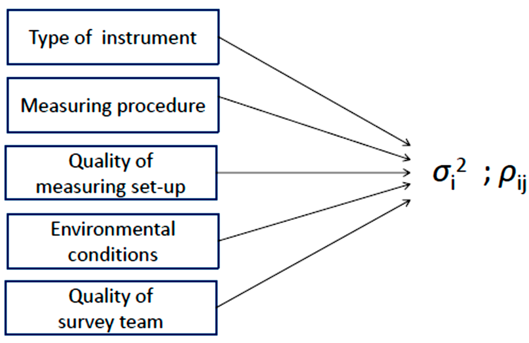
As outlined in the last section, the traditional statistical concept, which derives dispersion measures and correlations out of repeated independent (!) observations, does not cover the complexity of today’s measuring processes, see Figure 1.
Considering the deficiencies within the classical error theory, on initiative of the Bureau International des Poids et Mesures, France, an international group of experts of metrology formed in 1987 to develop a new approach to adequately assess the complete uncertainty budget of different types of measurements. As a result, the “Guide to the Expression of Uncertainty in Measurement” (GUM) was published, which nowadays is the international standard in metrology, see the fundamental publications [1,2]. The GUM allows the computation of uncertainty quantities for all measuring sensors or systems. The resulting uncertainty value is a non-negative parameter characterizing the complete dispersion of a measuring quantity and by this, nowadays, uncertainty values are considered to be the adequate precision parameters.
As described in the fundamental GUM documents, it is necessary to model the complete measuring and processing chain to derive a “final” resulting measuring quantity from all influencing raw data. It is important that this numerical model includes all, and really all, input quantities , , …, that influence the final measuring result . As this model contains all the computational steps, including how the resulting quantity will be changed whenever one input quantity is modified, this basic model for GUM analysis is named carrier of information. In a simplified form, this model can be described as a (often nonlinear) complex function
The development of this function is one of the most difficult and complex subtasks for deriving the uncertainty of measurements. Deep understanding of the physical and computational processes within the sensor, the performance of the measuring task itself, the data processing and possible external and environmental influences are necessary. To do this, no standard concept is available, just some recommendations can be given, see e.g., [6,7].
With respect to the later discussions here, it should be mentioned that the original GUM is going to derive an uncertainty measure for just one measuring quantity .
To restrict the contents of this paper, possible variabilities of the measurand—the physical quantity of interest, which is measured—is not considered here; as for this task, detailed physical knowledge of the specific object would be required.
3.2. Type A and Type B Influence Factors
An uncertainty analysis according to GUM has a probabilistic basis, but also aims to include all available knowledge of the possible factors that may influence the measuring quantity. Consequently, it is most important to set-up the following two types of influence factors, which are characterized as Type A and Type B:
- Type A: Dispersion values for measurements
- -
- Derived from common statistical approaches, i.e., analyzing repeated observations;
- -
- Values following Gaussian distribution.
- Type B: Non-statistical effects
- -
- What are relevant external influences?
- -
- Are there remaining systematic effects?
- -
- Are insufficient formulas used during processing?
- -
- Define possible variability within specified interval [a, b];
- -
- Assign a probability distribution to each influence factor.
The GUM concept allows us to consider classical random effects (Type A) on measuring results, which correspond to established statistical approaches.
However, additionally, GUM allows us to include all relevant additional influence factors (Type B), e.g., external effects (e.g., due to environmental conditions and the observing team) and possibly remaining systematic errors (e.g., uncontrolled residuals from the measuring procedure, undetected instrumental effects). Even approximations used in computational formulas have to be considered, and as such, are considered here.
3.3. Assignment of Adequate Probability Distribution Functions to Variables
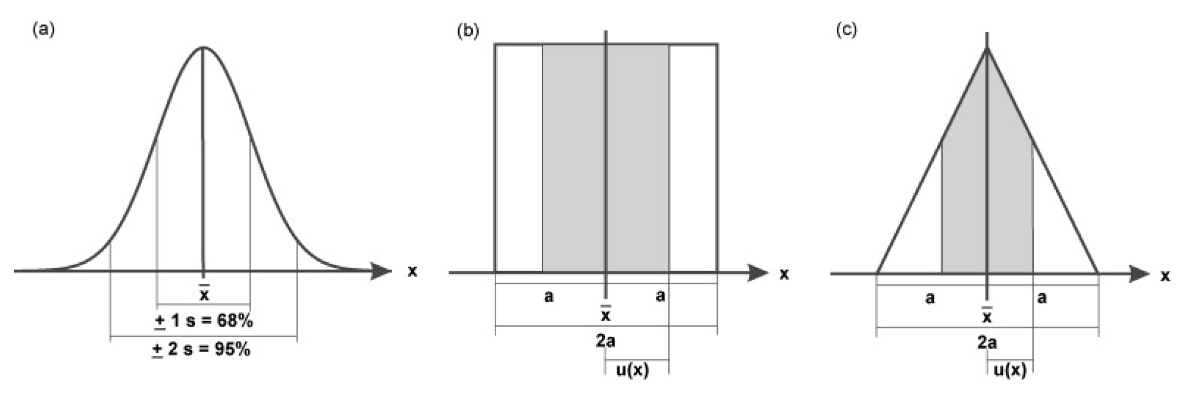
The GUM concept requires the assignation of statistical distribution functions for all these influencing quantities of Type A and Type B, i.e., a specific distribution, its expectation and dispersion. This aspect is depicted in Figure 2.
For Type A quantities, the common probability distribution functions with Gaussian or Normal distribution (with parameter expectation and variance ) are applied, which is depicted in Figure 2a. Here, classical methods for variance estimation can be used, i.e., the statistical analysis of repeated measurements from our own or external experiences, adopt data sheet information, etc.
For the non-statistical influence factors of Type B, which represent external influences and remaining systematic effects as well as insufficient approximations, according to, e.g., [9,10], it is recommended to introduce a probability distribution function in addition. However, the individual assignment of an adequate statistical distribution is a particularly complex task; in general, the statistical concepts of normal, uniform and triangle distribution functions are used, see Figure 2 and examples in Table 1.
For each influence factor, a statistical distribution has to be defined with an expected mean and dispersion, i.e., all these quantities have to be pre-selected to serve as starting values for a complete GUM analysis. To be more specific, it is the engineers’ task to estimate the variability of the applied temperature correction during the measuring period, to estimate a quantity for the centering quality, to evaluate the correctness of calibration parameters, etc.
3.4. Approach to Perform a GUM Analysis for Geodetic Observations
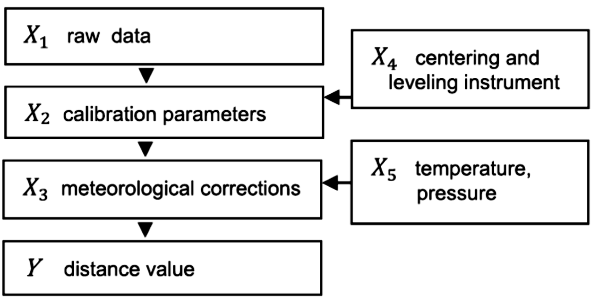
For Electronic Distance Measurements (EDMs), a common geodetic measuring technique, the processing steps according to Equation (9) are depicted in Figure 3. Be aware that here, the complete mathematical formulas are not given, just the specific computational steps are outlined.
The resulting distance value Y, i.e., the numerical measuring quantity after all necessary pre-processing steps, will serve as the input quantity for network adjustment, see Section 4.2. Within the classical approach, it is necessary to assign a dispersion value to this quantity, see Section 2.3, but here, as an alternative, Monte Carlo simulations are applied.
A simplified numerical example for the set-up of Type A and Type B effects is given in Table 1, where the used geodetic measurements can be applied in a local 3D geodetic network. However, each project requires an individual evaluation of these more general reference values; note, for the numerical example in Section 5, we had to make slight changes of these reference values to account for specific measuring conditions.
The here listed influencing factors of Type A and Type B, as well as their corresponding probability distribution functions and domain of variability, do not claim to be complete, as they do not contain additional computational influences related to the reduction to a reference height (which is always required), effects to account for the selected surveying methods, the quality of the personal or the atmospheric and environmental influences, such as bad weather, strong insolation, etc.
The here presented selection of the distribution type and its variability range are solely preliminary steps. At minimum, a GUM analysis of GNSS observations, a much more detailed study of all influencing factors, has to be performed, which is a current project at the Finish Geodetic Institute [12].
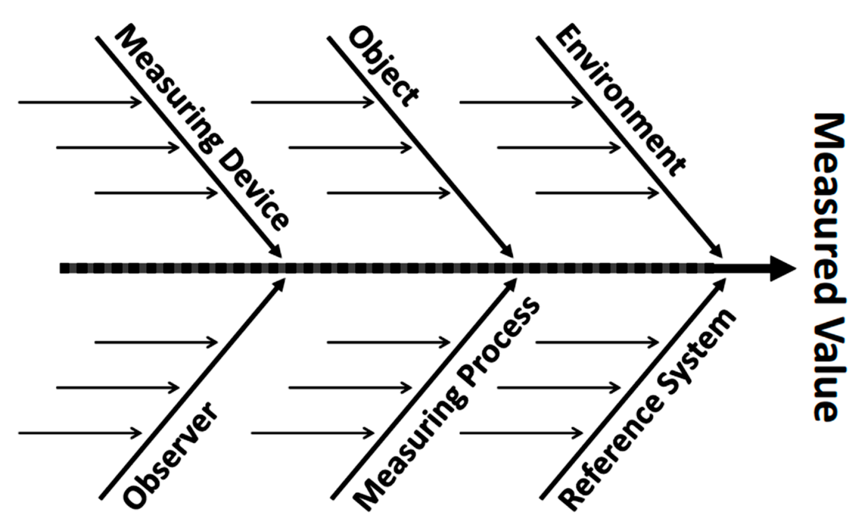
The algorithmic complexity of the set-up of Equation (9), i.e., the difficulty to find the relevant carrier of information, makes it necessary to analyze the complete measuring process and all pre-processing steps. This problem can be visualized in a so-called Ishikawa diagram, as given in Figure 4. This frequently applied diagram, see [13], has to be filled out for each specific measurement system, which can be a laborious task, e.g., the actual publication [14].
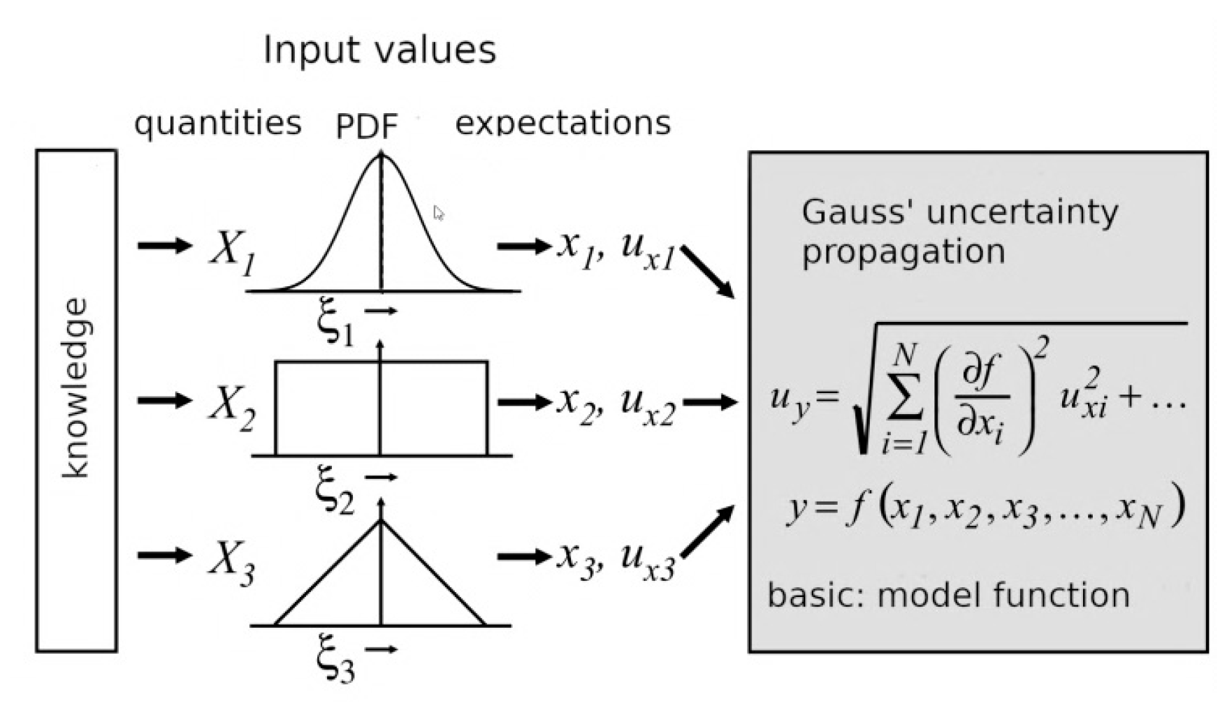
3.5. Uncertainty Quantities out of GUM
To combine all these effects of Type A and Type B within the classical GUM approach, the well-known law of variance propagation is applied, despite the fact that these are effects with different probability distribution functions. In Figure 5, this approach is explained: On the left-hand side, the different Probability Distribution Functions (PDF) are visualized, i.e., normal, uniform and triangle distribution. On the right-hand side, the formula for the law of variance propagation is shown, combining different uncertainties of Type A and Type B. Of course, for each influence factor an individual element has to be considered.
Numerically therefore, the uncertainty for the final measuring quantity , see Equation (9), is derived by combining the uncertainties of Type A () and Type B () for all influence factors following the formula:
Within GUM an extended and a complete uncertainty is introduced as well, both derived quantities out of . A discussion of the usefulness of these extensions and their computations is outside the scope of this paper.
3.6. Criticism
The application of statistical distribution functions to Type B errors and the application of the law of variance propagation to obtain an uncertainty estimate are critical points within the GUM approach [15]. The assignment of probability distribution functions to the influencing factors is a sensitive step and of course, the application of the law of variance propagation is a practical method, but it allows us to stay with the established statistical methods and perform subsequent computations.
This GUM concept is discussed within recent geodetic literature to some extent, see e.g., [13,14,15,16,17]. However, most of these discussions and critical remarks are limited to an uncertainty assessment for single measurements, not for complex networks or systems.
Taking into account this criticism, in a later extension of the GUM concept [2,3,18], the use of Monte Carlo simulations is recommended to find the final distribution for the quantity .
We will not follow this concept, but extend the processing model, see Figure 6, to directly study the stochastic properties of the outcome of the least squares adjustment. Due to our knowledge, such a network approach has not been considered yet.
4. Monte Carlo Simulations
4.1. Basic Idea of MC Simulations
For decades, Monte Carlo (MC) methods have been developed and in use to solve complex numerical problems in a specific way, i.e., by repeated random experiments, performed on a computer, see e.g., [19]. All MC computations use repeated random sampling for input quantities, process these input data according to the existing algorithms and obtain a variability of numerical results. For typical simulations, the repeat rate of experiments is 1000–100,000 or more, in order to obtain the most probable distribution of the quantities of interest. This allows MC simulations to model phenomena with well-defined variability ranges for input variables.
Nowadays, with modern computers and well-established Random Number Generators (RNG), large samples are easy to generate, see [20,21]. According to the variability of input quantities, pseudorandom sequences are computed, which allows us to evaluate and re-run simulations.
In this paper, MC simulations are applied to perform uncertainty modelling according to GUM, the specific case of geodetic data processing, i.e., network adjustment following a traditional Gauss–Markov (GM) model. The use of MC simulations allows us to include different Type A and Type B influence factors, which is an extension in relation to the classical approach. The approach allows us to combine a detailed GUM analysis of the measurement process with MC simulations in a rigorous way.
The typical pattern of an MC simulation is as follows:
- -
- Define functional relations between all input data and the quantities of interest.
- -
- Define probability distribution functions and variability ranges for starting data.
- -
- Generate corresponding input data with RNG.
- -
- Perform deterministic computations with these input values and obtain a pre-set number of realizations for the quantities of interest.
- -
- Analyze the achieved quantities of interest.
4.2. Concept to Combine MC-Simulations with GUM Analysis
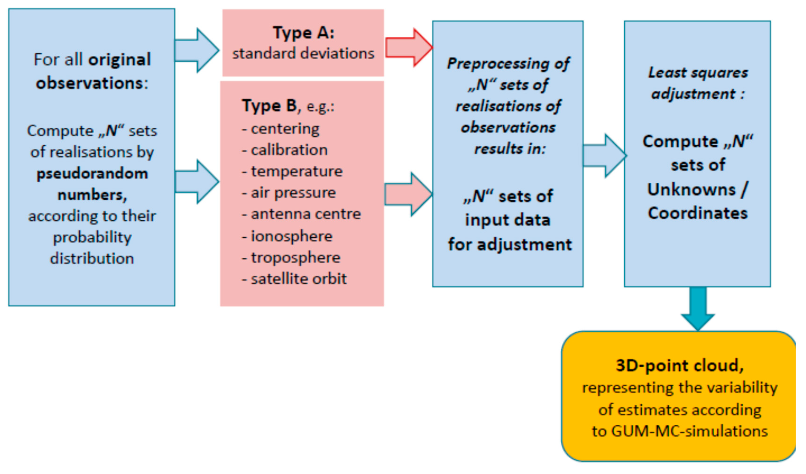
The scheme for the here proposed approach for an uncertainty assessment within least squares adjustments of geodetic networks by a rigorous combination of MC simulations with GUM analysis is presented in Figure 6. Starting point is an analysis of the complete pre-processing chain for each observation according to GUM, i.e., an analysis of all possible influencing factors of Type A and Type B, according to the important carrier of information formula, see Equation (9). For all these influencing factors, the most probable numerical measuring value is the starting point, often a mean value or a real observation.
As the next step, pseudorandom numbers for all influencing factors for each observation are created, taking into account their most probable value, the selected probability distribution function and the variability domain. There are numerous options for selecting a Random Number Generator (RNG). RNG should have high quality, i.e., provides good approximations of the ideal mathematical system, e.g., has long sequences, shows no gaps in data, fulfils distribution requirements, see [21]. As discussed in [20], the RANLUX (random number generator at highest luxury level) and its recent variant RANLUX++, which are used here, can be considered as representative of such high-quality RNGs.
For each original reading, respectively, for each influence factor, by using this RNG, a random value is created, representing one realization of the real measuring process. By combining these effects in a consecutive way, see the simplified example in Table 2, for each input quantity for network adjustment, such a randomly generated value is gained. With each set of input data, one least squares adjustment is performed, coming up with one set of coordinate estimates as the outcome.
Repeating this complete approach for a preset number of (e.g., 1000 or 10,000) simulations, the final results of a GUM-MC simulation are achieved, i.e., a set of coordinates/unknowns with its variability, which represent the uncertainty of the coordinates according to the used GUM analysis.
As an example, the specific manner, in which the random numbers for distance observations as input quantities for the adjustment are derived, are depicted in Table 2. Starting with a most probable mean value, such as Type B errors, the effects of pillar variations, calibration and weather and the classical Type A errors are considered. In column 2 their stochastic properties are given, which are the basis for the generation of a random number, which results in a specific modification of the distance observation, see column 3.
5. Application to a Local 3D Geodetic Network
5.1. Test Site “Metsähovi”
The Metsähovi Fundamental Station belongs to the key infrastructure of Finnish Geospatial Research Institute (FGI). Metsähovi is a basic station for the national reference system and the national permanent GNSS network. This station is a part of the global network of geodetic core stations, used to maintain global terrestrial and celestial reference frames as well as to compute satellite orbits and perform geophysical studies.
Of special interest here is the character of this network to serve as “Local Tie-Vector”, see [22], which is defined as a 3D-coordinate difference between the instantaneous phase centers of various space-based geodetic techniques, in this case between VLBI (Very Long Baseline Interferometry), GNSS (Global Navigation Satellite System) and SLR (Satellite Laser Ranging). All these techniques have different instruments on the site and the geometric relations between their phase centers have to be defined with extreme precision.
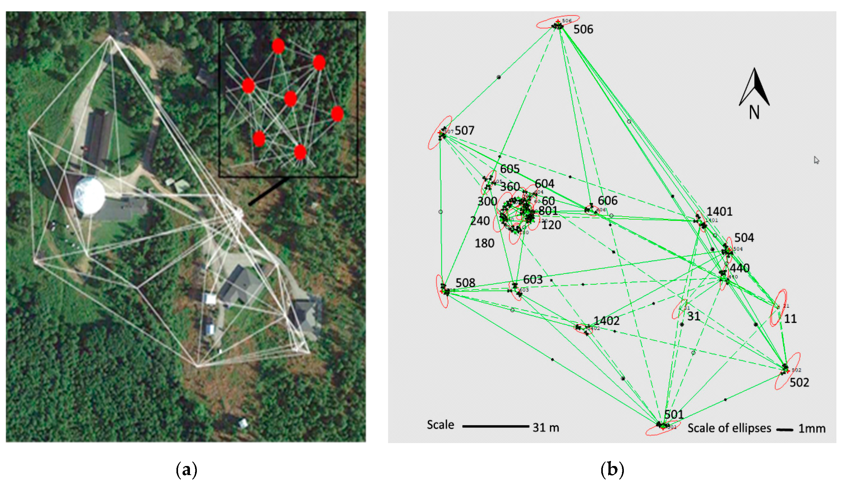
As depicted in Figure 7, the structure of this network is rather complex, a special difficulty is that the VLBI antenna is located inside a radome. This requires a two-step network with a connection between an outside and inside network, which is the most critical part in the network design, but this will not be discussed here in detail.
As already discussed in [11], the local tie network Metsähovi consists of 31 points, where specific local tie vectors are given by the GNSS stations, 11 and 31, on the one hand side and point 180, which is located within a radome. This station 180 is not the reference point of the VLBI antenna, it is located in its neighborhood. Here, a 3D free network adjustment is performed with the following measurement elements: 149 total station measurements (slope distances, horizontal directions and vertical angles), 48 GNSS baselines and levelled 43 height differences.
5.2. Input Variables for GUM Analysis
To get a realistic idea of uncertainties within this network, a classical adjustment model, which combines GNSS, total station and levelling measurements, is set up for this Metsähovi network. Then, all (many) influence factors are considered according to a GUM analysis. The Monte Carlo simulation process starts with the generation of pseudo random numbers for the influence factors, resulting in a set of input values for the adjustment. Repeating this MC simulation with 1000 runs gives the here discussed results.
The GNSS uncertainty model is just a rough idea, as in general it is difficult to simulate all influence factors with e.g., orbital errors, remaining atmospheric effects, multipath and near field effects. Colleagues from FGI are working on the problem to develop a more realistic GUM model for GNSS, see [12].
In our approach, the local tie network is simulated with 1000 runs of pre-analysis and least squares adjustment. In each run, a new set of observations is generated and subsequently a new set of station coordinates is computed. A forced centering is assumed, therefore, in each simulation the coordinates may differ only according to possible pillar centering variations.
The local tie vector consists of the outside stations 11 and 31 and station 180 in the radome, see above. The uncertainty estimates for these stations will be considered here in detail.
According to the GUM concept, the following influencing factors were considered. As mentioned in Section 3.4, some changes of the reference values in Table 1 were necessary to account for specific measurement conditions.
5.2.1. Type A: Classical Approach, Standard Deviations
Total station observations
As standard deviation for modern total stations (e.g., Leica TS30) often values of 0.15 mgon for manual angle measurements and of 0.3 mgon for observations with automatic target recognition are used. With two sets of angle observations, a precision of 0.2 mgon is assumed to be valid:
- -
- Horizontal directions: normal distribution, = 0.2 mgon;
- -
- Zenith angles: normal distribution, = 0.2 mgon;
- -
- Slope distances: normal distribution, = 0.6 mm + 1 ppm.
GNSS Baselines
In these computations just a rough estimate is used, neglecting correlations between baseline components:
- -
- For each coordinate component: normal distribution, = 3.0 mm.
Height differences
- -
- Height differences: normal distribution, = 2.0 mm/.
5.2.2. Type B: Additional Influences, including Systematic Effects, External Conditions, Insufficient Approximations, etc.
Variation of pillar and centering
- -
- Uniform distribution, range: 0–0.1 mm.
Variation of instrument and target height
- -
- Uniform distribution, range: 0–0.1 mm.
Effects of calibration (total station instrument)
Schwarz [14] gives possible standard deviations of calibration parameters for total stations:
- -
- Additive constant: normal distribution, = 0.2 mm (valid for combination of instrument and specific prism).
- -
- Scale unknown: normal distribution, = 0.8 ppm. The value for scale is related to the problem to determine a representative temperature along the propagation path of the laser beam.
Effect of calibration of GNSS antenna
- -
- Not implemented yet because these effects were not known to us for the test site Metsähovi.
Effects of limited knowledge on atmospheric parameters
- -
- Air temperature: uniform distribution, range 0–0.8 K; (effect: 1 K ≈ 1 ppm);
- -
- Air pressure: uniform distribution, range 0–0.5 mbar; (effect: 1 mbar ≈ 0.3 ppm);
- -
- Air humidity: uniform distribution, range 0–5%.
5.3. Final Results of GUM-Analysis and MC Simulations
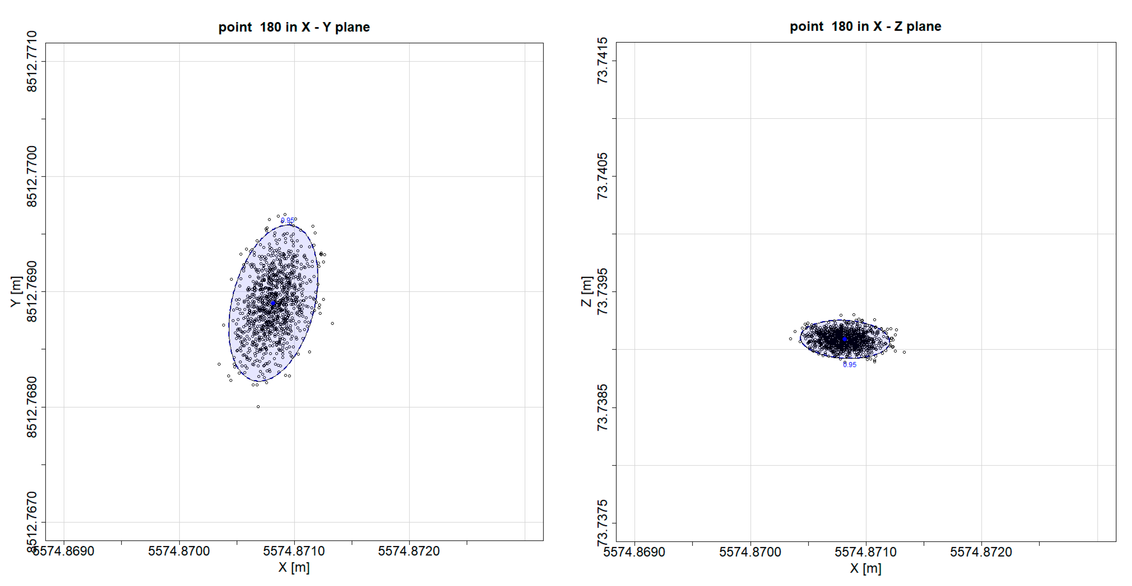
We applied to this network the developed approach of detailed GUM analysis and full MC simulation, i.e., starting with a simulation of the original influence factors and then performing an adjustment. In Figure 8 and Figure 9, the resulting point clouds are depicted for coordinates for stations 11, 31 and 180, which form the local tie vectors. As the Metsähovi network is a 3D geodetic network, for simplicity the resulting point clouds are visualized in the X–Y plane and X–Z plane.
This variation of all coordinate components is of special interest here, as the local tie vectors are defined between the GPS Reference stations 11 and 31 and station 180 inside the radome. The original coordinate differences refer to the global cartesian coordinate system.
6. On Stochastic Properties of These Point Clouds
The focus of this paper is the stochastic properties for the results of such a MC simulation where the input data are randomly variated quantities, following the GUM analysis concept, see the scheme in Figure 6 and the description given in Section 4.2.
For this analysis, we consider the point clouds for final coordinates as information of primary interest, as depicted e.g., in Figure 8 and Figure 9, separated into X-Y and X-Z planes to make it easier to visualize the findings. To study the stochastic properties of these results, two concepts from mathematical statistics can be considered.
6.1. Cramér’s Central Limit Theorem
Already in 1946, the statistician Cramér [23] developed a probabilistic theory, which is well-known as the Central Limit Theorem (CLT). Without going into detail, the general idea of the CLT is, that the properly normalized sum of independent random variables tends towards a normal distribution, when they are added. This theorem is valid, even if it cannot be guaranteed that the original variables are normally distributed. This CLT is a fundamental concept within probability theory because it allows for the application of probabilistic and statistical methods, which work for normal distributions, to many additional problems, which involve different types of probability distributions.
Following Section 4.2, during the GUM analysis a number of influence factors with different distributions are combined, what is of course more than the “properly normalized sums”, which are asked for in the CLT. However, the question is whether or not the resulting input variables of the adjustment are sufficiently normal distributed or—considered here—if the resulting point clouds after MC simulations for adjustment using these input datasets tend to have a normal distribution.
6.2. Hagen’s Elementary Error Theory
Within geodesy and astronomy, a theory of elementary errors was already developed by Hagen in 1837 [24]. This concept means that randomly distributed residuals , for which we assume the validity of a normal distribution, can be considered to be the sum of a number of very small elementary errors :
This equation holds—according to Hagen’s discussion—if all elementary errors have similar absolute size and positive and negative values have the same probability.
Of course the conditions for this theory are not really fulfilled by the here considered concept of GUM analysis of influence factors with subsequent MC simulation, but out of this elementary error theory one could ask whether or not the results of the here proposed approach tends to have a normal distribution, as well.
6.3. Test of MC Simulation Results on Normal Distribution
To analyze the statistical distribution of a sample of data, numerous test statistics are developed. For analyzing the normal distribution, here we used the test statistics of Shapiro–Wilks, Anderson–Darling, Lilliefors (Kolmogorov–Smirnov) and Shapiro–Francia. A detailed description of these test statistics is given in the review article [25]. The principle of all these tests is to compare the distribution of empirical data with the theoretical probability distribution function.
Here, we want to perform one-dimensional tests for the variation of the x-, y- and z-components of the stations 11, 31 and 180 of our reference network Metsähovi. The used coordinates are the results of 1000 MC simulations, where the input data are pre-processed according to the concept of Section 4.2.
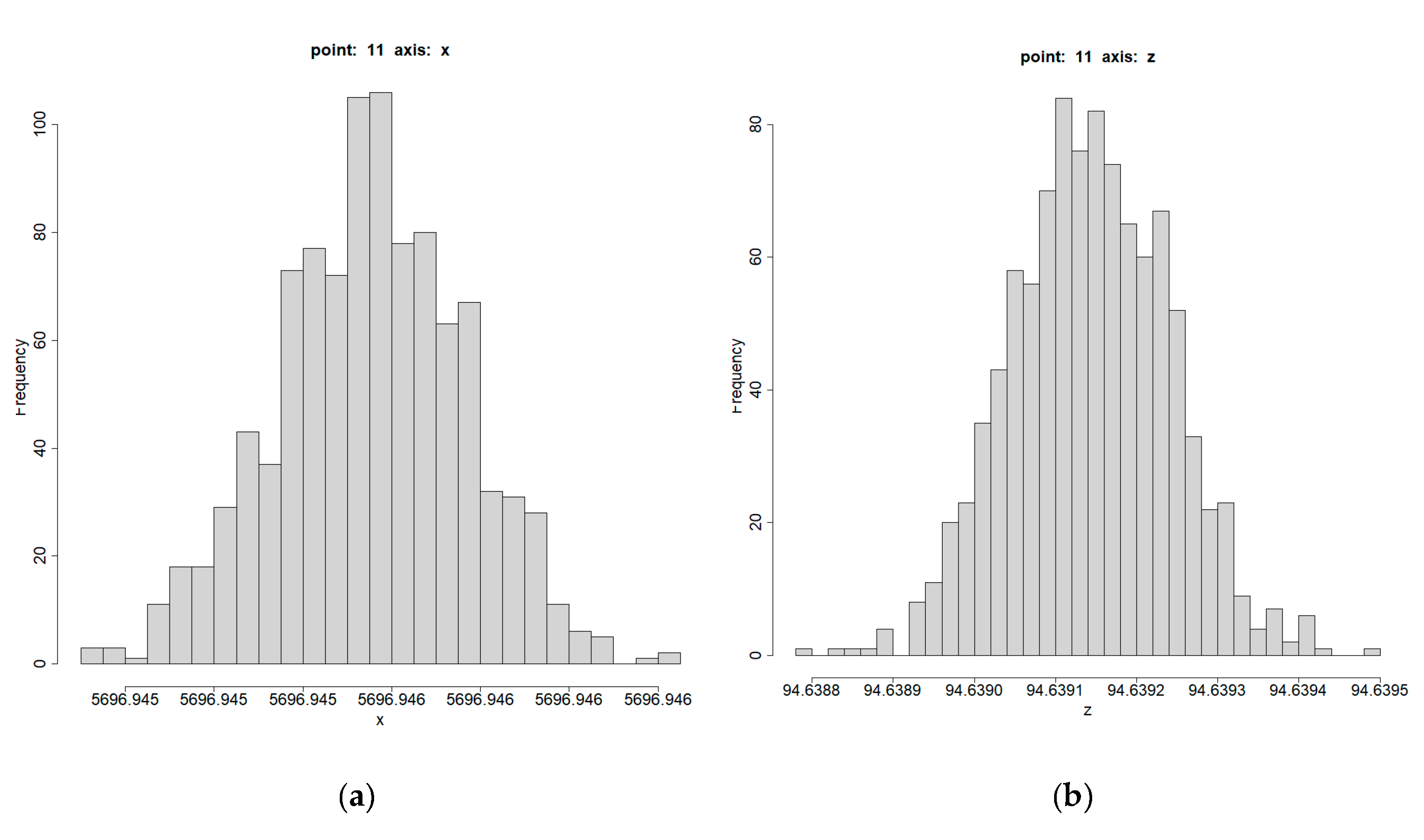
The above-mentioned numerical tests for these simulated values accept for all stations the hypothesis of normal distribution. For us, this is an indication that should be allowed in order to consider the results of the here proposed approach of having a normal distribution. This means an uncertainty for station coordinates, derived via GUM analysis and subsequent MC simulation, can be treated for ongoing statistical analysis of results, such as general quality assessment and deformation analysis, in the same way as the results of classical adjustment. Some additional graphical information for these comparisons can be given, as well. In Figure 9, the distribution of the x- and z-components of station 11 are depicted, received from least squares adjustments after GUM and MC simulations, i.e., corresponding the results of Figure 8. It is obvious that the appearance of the components is close to the well-known bell curve of normal distribution. For the stations 31 and 180 these distributions were visualized, as well, with very similar appearances.
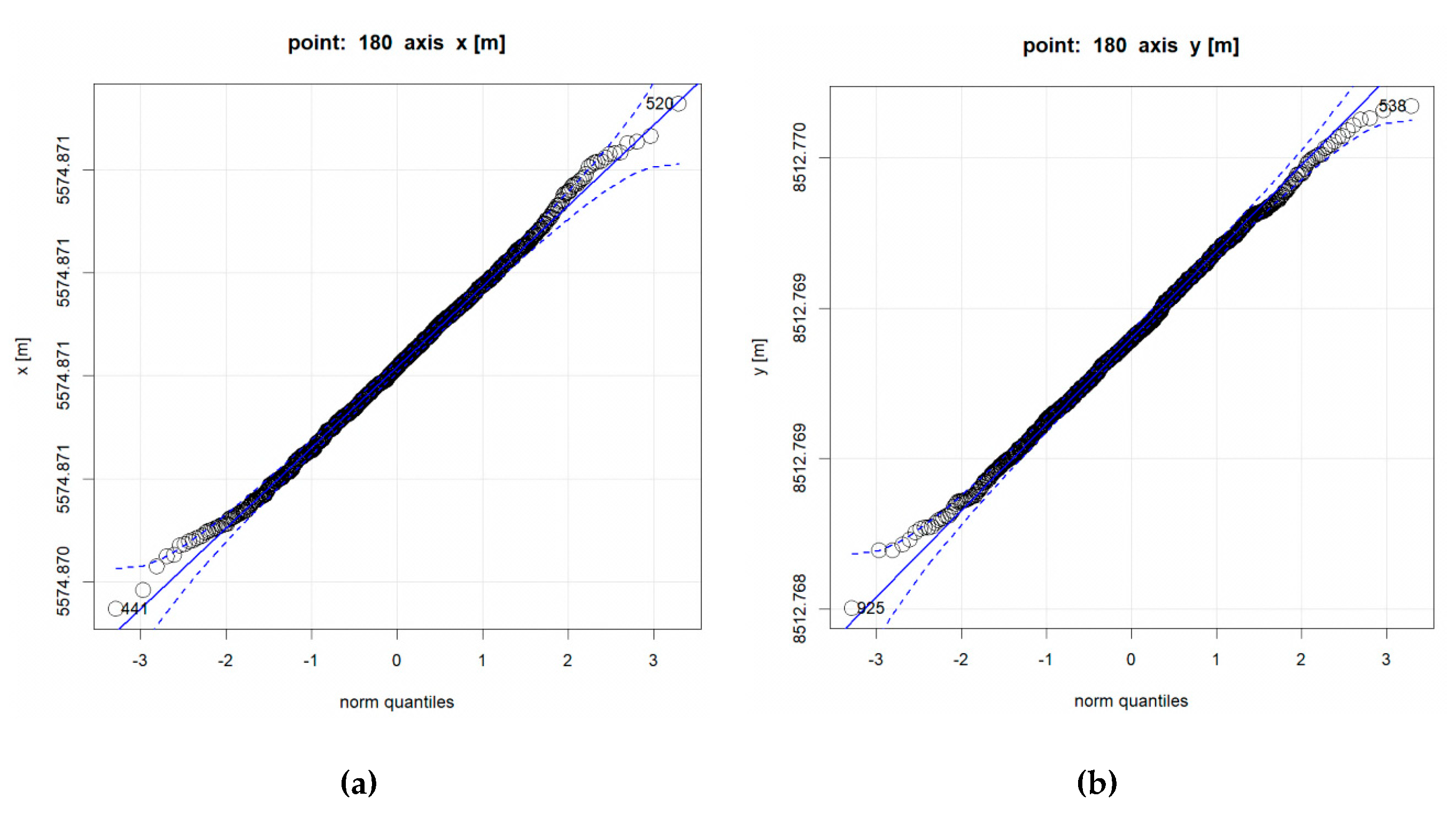
The Q–Q (quantile–quantile) plot is a graphical method for comparing two probability distributions by representing their quantities in a plot against each other. If the two distributions being compared are similar, the points in the Q–Q plot will approximately appear in a line.
If the most real points are within the dashed line, here representing a normal distribution, the assumption of a normal distribution is allowed. The confidence level for point-wise confidence envelope is 0.95. From Figure 10, it can be seen that for station 180 a normal distribution can be accepted. For stations 11 and 31, the assumption of a normal distribution is accepted, as well.
7. Conclusions
Within the classical approach of network adjustment, see e.g. [4,5], more or less rough and subjective estimates for the dispersion of measurements are introduced. A detailed criticism to this approach is given in Section 2.4. The here described GUM-based approach starts with an analysis of the complete measuring process and computational process, i.e., it considers all influence factors, which are used during the pre-processing steps. By this, the GUM approach can be considered to give more realistic quantities for the precision of the input data of an adjustment of geodetic networks.
Using random numbers to cover the variability of these input data allows us to perform Monte Carlo simulations, which makes it possible to compute the corresponding variability or uncertainty ranges of final coordinate sets.
These variations are analyzed statistically and tend to follow a normal distribution. This allows us to derive confidence ellipsoids out of these point clouds and to continue with classical quality assessment and more detailed analysis of results, as is performed in established network theory.
Of course, these results are dependent on the selection of the statistical distributions and their variability domains during the GUM analysis of the relevant Type A and Type B influence factors. This concept allows a new way of analyzing the effects of all influence factors on the final result, i.e., the form and size of derived ellipsoids. For example, one can analyze the effect of a less precise total station or a better GNNS system the same way one can study the influence of limited knowledge of the atmospheric conditions or a more rigorous centering system. These studies are outside the scope of this paper. Anyway, the here proposed approach allows a straightforward application of the GUM concept to geodetic observations and to geodetic network adjustment. Being optimistic, the here presented concept to derive confidence ellipsoids out of GUM–MC simulations could replace the classical methods for quality assessment in geodetic networks. The GUM approach will lead to uncertainty estimates, which are more realistic for modern sensors and measuring systems and it is about time to adapt these new concepts from metrology within the discipline of geodesy.
Author Contributions
Conceptualization, methodology and writing: W.N.; formal analysis, software development, visualization and review: D.T. Both authors have read and agreed to the published version of the manuscript.
Funding
Preliminary work for this project is performed within the frame work of the joint research project SIB60 “Surveying” of the European Metrology Research Programme (EMRP). EMRP research is jointly funded by the participating countries within EURAMET and the European Union. The analysis of stochastic properties, presented here, has not received external funding.
Acknowledgments
The authors have to thank the company Geotec Geodätische Technologien GmbH, Laatzen, Germany, for allowing us to use a modification of their commercial software package PANDA for carrying out all computations presented here.
Conflicts of Interest
The authors declare no conflict of interest.
References
- JCGM (100:2008): Evaluation of Measurement Data—An Introduction of the “Guide to the Expression of Uncertainty in Measurements”. Available online: https://www.bipm.org (accessed on 31 March 2020).
- JCGM (101:2008): Evaluation of Measurement Data-Supplement 1 “Guide to the Expression of Uncertainty in Measurement” Propagation of Distributions Using a Monte Carlo Method. Available online: https://www.bipm.org (accessed on 2 April 2020).
- Bich, W. Uncertainty Evaluation by Means of a Monte Carlo Approach. In Proceedings of the BIPM Workshop 2 on CCRI Activity Uncertainties and Comparisons, Sèvres, France, 17–18 September 2008; Available online: http://www.bipm.org/wg/CCRI(II)/WORKSHOP(II)/Allowed/2/Bich.pdf (accessed on 21 April 2020).
- Niemeier, W. Ausgleichungsrechnung, 2nd ed.; Walter de Gruyter: Berlin, Gemany, 2008. [Google Scholar]
- Strang, G.; Borre, K. Linear Algebra, Geodesy and GPS; Wellesley-Cambridge Press: Wellesley, MA, USA, 1997. [Google Scholar]
- Kessel, W. Measurement uncertainty according to ISO/BIPM-GUM. Thermochim. Acta 2002, 382, 1–16. [Google Scholar] [CrossRef]
- Sommer, K.-D.; Siebert, B. Praxisgerechtes Bestimmen der Messunsicherheit nach GUM. Tm Tech. Mess. 2004, 71, 52–66. [Google Scholar] [CrossRef]
- Meyer, V.R. Measurement Uncertainty. J. Chromatogr. A 2007, 1158, 15–24. [Google Scholar] [CrossRef] [PubMed]
- Sivia, D.S. Data Analysis-A Bayesian Tutorial; Clarendon Press: Oxford, UK, 1996. [Google Scholar]
- Weise, K.; Wöger, W. Meßunsicherheit und Meßdatenauswertung; Wiley-VCH Verlag GmbH & Co. KGaA: Weinheim, Germany, 1999. [Google Scholar]
- Niemeier, W.; Tengen, D. Uncertainty assessment in geodetic network adjustment by combining GUM and Monte-Carlo-simulations. J. Appl. Geod. 2017, 11, 67–76. [Google Scholar] [CrossRef]
- Kallio, U.; Koivula, H.; Lahtinen, S.; Nikkonen, V.; Poutanen, M. Validating and comparing GNSS antenna calibrations. J. Geod. 2019, 93, 1–18. [Google Scholar] [CrossRef] [Green Version]
- Hennes, M. Konkurrierende Genauigkeitsmasse—Potential und Schwächen aus sicht des Anwenders. Allg. Vermess. Nachr. 2007, 114, 136–146. [Google Scholar]
- Schwarz, W. Methoden der Bestimmung der Messunsicherheit nach GUM-Teil 1. Allg. Vermess. Nachr. 2020, 127, 69–86. [Google Scholar]
- Kutterer, H.-J.; Schön, S. Alternativen bei der Modellierung der Unsicherheiten beim Messen. Z. Vermess. 2004, 129, 389–398. [Google Scholar]
- Neumann, I.; Alkhatib, H.; Kutterer, H. Comparison of Monte-Carlo and Fuzzy Techniques in Uncertainty Modelling; FIG Symposium on Deformation Analysis: Lisboa, Portugal, 2008. [Google Scholar]
- Jokela, J. Length in Geodesy—On Metrological Traceability of a Geospatial Measurand; Publications of the Finnish Geodetic Institute: Helsinki, Finland, 2014; Volume 154. [Google Scholar]
- Siebert, B.; Sommer, K.-D. Weiterentwicklung des GUM und Monte-Carlo-Techniken. Tm Tech. Mess. 2004, 71, 67–80. [Google Scholar] [CrossRef]
- Kroese, D.P.; Taimre, T.; Botev, Z.I. Handbook of Monte Carlo Methods; Wiley & Sons: Hoboken, NJ, USA, 2011; Volume 706. [Google Scholar]
- James, F.; Moneta, L. Review of High-Quality Random Number Generators. In Computing and Software for Big Science; Springer Online Publications: Berlin/Heidelberg, Germany, 2020. [Google Scholar]
- Knuth, D.E. The Art of Computer Programming, Volume 2: Semi-Numerical Algorithms, 3rd ed.; Addison-Wesley: Reading, PA, USA, 1998. [Google Scholar]
- Ning, T.; Haas, R.; Elgered, G. Determination of the Telescope Invariant Point and the local tie vector at Onsala using GPS measurements. In IVS 2014 General Meeting Proceedings “VGOS: The New VLBI Network”; Science Press: Beijing, China, 2014; pp. 163–167. [Google Scholar]
- Cramér, H. Mathematical models in statistics. In Princeton Math. Series, 9th ed.; Princeton University Press: Princeton, NJ, USA, 1946. [Google Scholar]
- Hagen, G. Grundzüge der Wahrscheinlichkeitsrechnung; Verlag von Ernst&Korn: Berlin, Germany, 1837. [Google Scholar]
- Ogunleye, L.I.; Oyejola, B.A.; Obisesan, K.O. Comparison of Some Common Tests for Normality. Int. J. Probab. Stat. 2018, 7, 130–137. [Google Scholar]
Figure 1.
Set-up of a stochastic model within classical approach: external, instrumental and personal influences are considered “implicitly”, at least in a subjective way.
Figure 1.
Set-up of a stochastic model within classical approach: external, instrumental and personal influences are considered “implicitly”, at least in a subjective way.

Figure 2.
Statistical distribution functions, used within the Guide to the Expression of Uncertainty in Measurement (GUM) approach to model effects of Type A and Type B, from [8]. (a) Normal distribution, (b) uniform distribution and (c) rectangular distribution.
Figure 2.
Statistical distribution functions, used within the Guide to the Expression of Uncertainty in Measurement (GUM) approach to model effects of Type A and Type B, from [8]. (a) Normal distribution, (b) uniform distribution and (c) rectangular distribution.

Figure 3.
Influence factors for electronic distance measurements: processing steps for the derivation of an input quantity for an adjustment, from [11].
Figure 3.
Influence factors for electronic distance measurements: processing steps for the derivation of an input quantity for an adjustment, from [11].

Figure 4.
Ishikawa diagram to analyze all the influence factors for a GUM analysis.

Figure 5.
Classical concept to combine Type A and Type B influence parameters within GUM [7].
Figure 5.
Classical concept to combine Type A and Type B influence parameters within GUM [7].

Figure 6.
GUM concept for creation of “” sets of input data used in Monte Carlo (MC) simulations for least squares network adjustments.
Figure 6.
GUM concept for creation of “” sets of input data used in Monte Carlo (MC) simulations for least squares network adjustments.

Figure 7.
(a) Fundamental station Metsähovi, Finland, WGS84 (60.217301 N, 24.394529 E); with local tie network. (b) Network configuration with stations 11, 31 and 180, which define local tie vectors.
Figure 7.
(a) Fundamental station Metsähovi, Finland, WGS84 (60.217301 N, 24.394529 E); with local tie network. (b) Network configuration with stations 11, 31 and 180, which define local tie vectors.

Figure 8.
Point clouds of coordinate variations for stations 11, 31 and 180. Left: in X-Y plane. Right: in X-Z plane. The elliptical contour lines refer to a confidence level of 95%.
Figure 8.
Point clouds of coordinate variations for stations 11, 31 and 180. Left: in X-Y plane. Right: in X-Z plane. The elliptical contour lines refer to a confidence level of 95%.


Figure 9.
Histograms of the variations of (a) x- and (b) z-coordinates of station 11 after GUM and MC simulation.
Figure 9.
Histograms of the variations of (a) x- and (b) z-coordinates of station 11 after GUM and MC simulation.

Figure 10.
Q–Q plots for comparing probability distributions of (a) x- and (b) y-coordinates of station 180: If real values lie within dashed line, here assumed normal distribution is accepted.
Figure 10.
Q–Q plots for comparing probability distributions of (a) x- and (b) y-coordinates of station 180: If real values lie within dashed line, here assumed normal distribution is accepted.


Table 1.
Type A and Type B influencing factors, possible probability distribution functions and variability range for typical geodetic observations, taken from [11].
Table 1.
Type A and Type B influencing factors, possible probability distribution functions and variability range for typical geodetic observations, taken from [11].
| Influence Factors | Distribution | Examples | |
|---|---|---|---|
| Type A | Total station | ||
| - horizontal directions - vertical distances - slope distances | normal normal normal | = 0.2 mgon = 0.3 mgon = 0.6 mm + 1 ppm | |
| Levelling | |||
| - height differences | normal | = 0.6 mm/ | |
| GNSS | |||
| - baselines | normal | = 2 mm | |
| Type B | Pillar und centering | ||
| - centering direction - centering offset - Target center definition | uniform triangle uniform | [0, 360°] [0, 0.1 mm] = 0.1 mm | |
| Instrument and target height | uniform | [0, 0.2 mm] | |
| Calibration parameters | |||
| - additional constant - scale factor | normalnormal | = 0.5 mm = 0.2 ppm | |
| Atmospheric parameters | |||
| - temperature - air pressure - air humidity | uniform uniform uniform | [0, 1 K] [0, 1 mbar] [0, 5%] | |
GNSS, Global Navigation Satellite System.
Table 2.
Derivation of one input quantity for a distance, using random numbers for some influencing effects.
Table 2.
Derivation of one input quantity for a distance, using random numbers for some influencing effects.
| Action | Stochastic Properties | Resulting in Random Distance Value: |
|---|---|---|
| “True” coordinates | = 100.0000 m, = 100.0000 m = 200.0000 m, = 200.0000 m | |
| + Pillar variations result in: “real distance” | Uniform distribution: σ = 0.1 mm | = 100.00005 m, = 99.99999 m = 199.99998 m, = 200.00001 m = 141.42132 m |
| + Calibration effects | ||
| additional constant: | Normal distribution: σ = 0.5 mm | |
| scale | Normal distribution: σ = 1 ppm | = 141.42165 m |
| + Weather effects | ||
| temperature | Uniform distribution: σ = 1 K | |
| air pressure | Uniform distribution: σ = 5 mbar | = 141.42163 m |
| + Type A uncertainties | ||
| Constant effect | Normal distribution: σ = 0.6 mm | |
| Distance dependent | Normal distribution: σ = 1 ppm | = 141.42136 m |
© 2020 by the authors. Licensee MDPI, Basel, Switzerland. This article is an open access article distributed under the terms and conditions of the Creative Commons Attribution (CC BY) license (http://creativecommons.org/licenses/by/4.0/).
Share and Cite
MDPI and ACS Style
Niemeier, W.; Tengen, D. Stochastic Properties of Confidence Ellipsoids after Least Squares Adjustment, Derived from GUM Analysis and Monte Carlo Simulations. Mathematics 2020, 8, 1318. https://doi.org/10.3390/math8081318
AMA Style
Niemeier W, Tengen D. Stochastic Properties of Confidence Ellipsoids after Least Squares Adjustment, Derived from GUM Analysis and Monte Carlo Simulations. Mathematics. 2020; 8(8):1318. https://doi.org/10.3390/math8081318
Chicago/Turabian StyleNiemeier, Wolfgang, and Dieter Tengen. 2020. "Stochastic Properties of Confidence Ellipsoids after Least Squares Adjustment, Derived from GUM Analysis and Monte Carlo Simulations" Mathematics 8, no. 8: 1318. https://doi.org/10.3390/math8081318
Note that from the first issue of 2016, this journal uses article numbers instead of page numbers. See further details here.