3D Dilatometer Time-Series Analysis for a Better Understanding of the Dynamics of a Giant Slow-Moving Landslide


1
Institute of Rock Structure and Mechanics, The Czech Academy of Sciences, V Holešovičkách 94/41, 18200 Prague, Czechia
2
Research Institute of Geodesy, Topography and Cartography, Ústecká 98, 25066 Zdiby, Czechia
3
Centro Geofísico de Canarias, Instituto Geográfico Nacional, Calle la Marina 20, 38001 Santa Cruz de Tenerife, Spain
*
Author to whom correspondence should be addressed.
Appl. Sci. 2020, 10(16), 5469; https://doi.org/10.3390/app10165469
Submission received: 30 June 2020
/
Revised: 28 July 2020
/
Accepted: 3 August 2020
/
Published: 7 August 2020
(This article belongs to the Special Issue Novel Approaches in Landslide Monitoring and Data Analysis)
Abstract
:Featured Application
Analysis of monitoring data from very slow-moving landslides.
Abstract
This paper presents a methodological approach to the time-series analysis of movement monitoring data of a large slow-moving landslide. It combines different methods of data manipulation to decrease the subjectivity of a researcher and provides a fully quantitative approach for analyzing large amounts of data. The methodology was applied to 3D dilatometric data acquired from the giant San Andrés Landslide on El Hierro in the Canary Islands in the period from October 2013 to April 2019. The landslide is a creeping volcanic flank collapse showing a decrease of speed of movement during the monitoring period. Despite the fact that clear and unambiguous geological interpretations cannot be made, the analysis is capable of showing correlations of the changes of the movement with increased seismicity and, to some point, with precipitation. We consider this methodology being the first step in automatizing and increasing the objectivity of analysis of slow-moving landslide monitoring data.
1. Introduction
Analysis of monitoring data from very slowly moving landslides faces very difficult issues considering the precision and accuracy of the used monitoring instruments, the influence of the different environmental factors on the measured data, the frequency of the measurements and the overall complexity of the phenomena [1,2,3,4]. In the case of large landslides (of more than several km2) another problem arises with choosing the right placement of the monitoring devices on the ground, as remote sensing methods such as LiDAR or InSAR, despite their enormous applicability, still do not provide comparable sub-mm accuracy [5,6].
When analyzing the landslide movement monitoring results, the time-series analysis should be used. Time-series analysis comprises different statistical methods to understand the underlying context of data points or to make forecasts [7]. It can capture seasonal behaviors, trends and changes [8]. Time-series analysis is routinely applied in econometrics [9,10]. In geosciences, there is a constant use of time-series analysis within GNSS observations [11] or climatology [12]. Thus, it might be a bit surprising that in landslide science, time-series analysis studies are mostly related to remote sensing (SAR) data analysis [13,14,15]. To some point, this is not surprising as SAR data are available in defined time-steps and form an undisrupted time series, which is the basic assumption of the analysis. In the case of landslides studies, time-series analysis is usually focused on trend behavior, sudden changes and seasonality analysis [16,17,18]. The big advantage of time-series analysis methods lies in the possibility to make predictions of future behavior based on previous activity. This is especially important in landslide disaster management. Complex non-linear time series are ubiquitous in geosciences [19]. The recently developed adaptive regression models (used in this work) appear to offer good solutions in multivariate non-stationary time-series analyses [20].
In the era of Big Data, it is more and more possible to harvest/gather a large amount of environmental and geophysical data related to slope stability using a variety of sensors and systems with high precision [21,22], which can be used for interpreting and monitoring the results and finding correlations to understand the landslide activity. However, a recent study [23] highlighted that the observations are prohibitively site-specific, highly subjective and fail to account for the spatial variability and correlations in slope movements and common trigger factors.
The landslide movement is usually neither smooth nor continuous. There are changes in the nature of the observed monitoring data at certain moments (changes of speed or direction of movement, jump events). We assume that these changes (events) during the development of landslide movements are caused by extreme states of factors (triggers) affecting the landslide movement (i.e., seismicity, precipitation) [24].
In this paper, we analyzed data from precise 3D dilatometers installed on the detachment planes of a giant complex landslide in a volcanic environment. The time-series analysis was performed on 1D, 2D and 3D data projections using adaptive regression. The main aim of this work was to find a suitable methodology for evaluating the time series of micro-movements to find the changes in landslide movement (events) in them and then compare them with the time moments of extreme external conditions including available climatic and seismic data to find correlations with the possible triggers of the landslide activity. The aim was fulfilled by applying known methods and combining them to understand better the landslide behavior and its responses to possible influencing factors.
2. Study Area
This study takes place on the island of El Hierro, Canary Islands, Spain. El Hierro is a composed oceanic volcano with the oldest subaerial rocks having an age of 1.12 Ma. Its youngest subaerially exposed rocks are represented by the Rift Series, with a maximum age of 0.16 Ma [25]. Over the past 33,000 years, onshore eruptions have reoccurred approximately once every 1000 years [26]. The latest, ongoing phase of volcanism began around 2.5 ka [27]. Recently a period of intense seismic activity spanned from July 2011 [28] to 2014 [29]. During this period, an offshore eruption started on 10 October 2011 and finished in March 2012 [30]. A more detailed description of the geology of the island has recently been presented elsewhere [31,32].
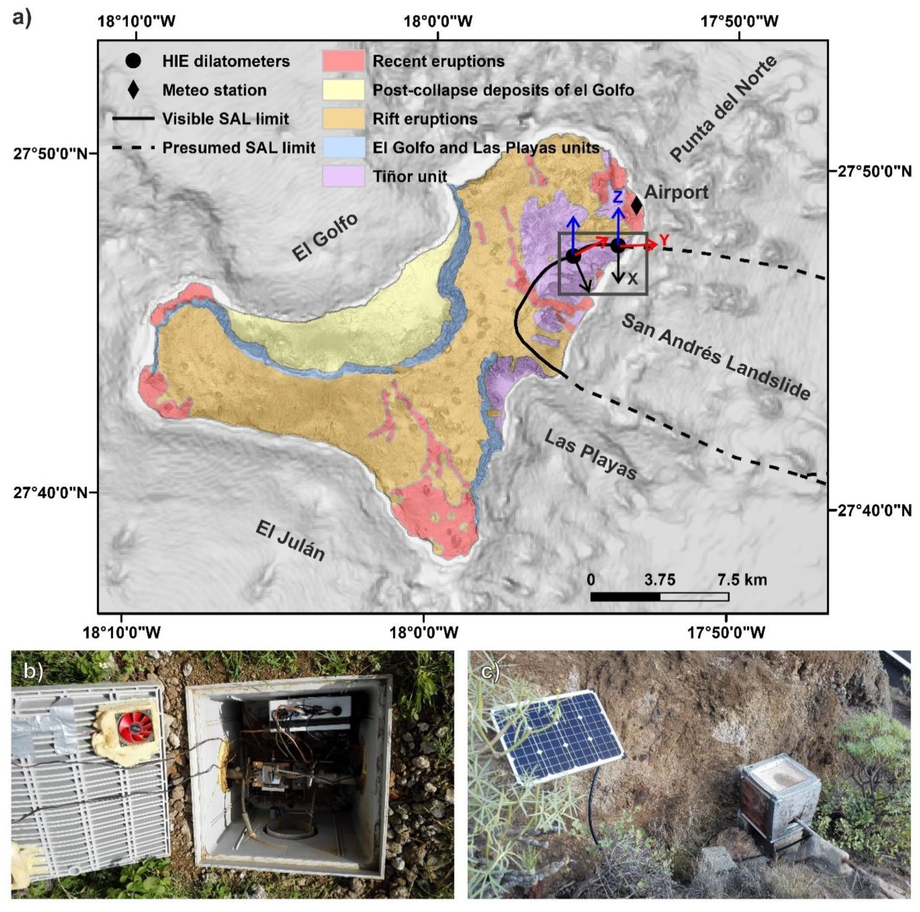
The characteristic three-point star morphology of El Hierro is a result of several enormous flank collapses (Figure 1). Until now, seven debris avalanches have been identified: Tiñor (<880 ka), Las Playas I (545–176 ka), Las Playas II (176–145 ka), El Julan (>158 ka), El Golfo A (176–133 ka), El Golfo B (87–39 ka), and Punta del Norte (unknown age) [27,33,34,35,36,37,38,39,40,41,42].
In addition to the previously mentioned flank collapses, a giant San Andrés Landslide (SAL) has been identified on the northeastern part of the island. The SAL is a deep-seated gravitational slope deformation [43] or a slump [44]. It has been supposed that the landslide underwent a single-event development at some point between 545 ka and 176 ka [45] and was inactive since then. Recent research shows, however, that there were at least two distinguishable separate slip events. The first one between 545 ka and 430 ka, and the second one between 183 ka and 52 ka [46]. Moreover, it has been proven that there is a continuous creep with a rate up to 0.5 mm·a−1, suggesting that the landslide mass may be moving steadily to the east and southeast [32,47,48]. Numerical stability modelling [49] showed that creep movements are possible due to unconsolidated sediments at the sea bottom, and destabilization of the landslide might be possible during periods of intense seismic activity.
This creep has been monitored by high-precision (±0.007 mm) 3D dilatometer gauges [3] with automatic data processing [50]. There are two devices installed on the landslide detachment plane in the upper scarp and on the left side of the landslide, respectively (Figure 1). The instrument records data based on optical−mechanical interferometry via the generation of moiré patterns, which result from the bending and interference of light rays as they pass through two specially designed optical grids [51].
3. Monitoring Data Collection and Preparation
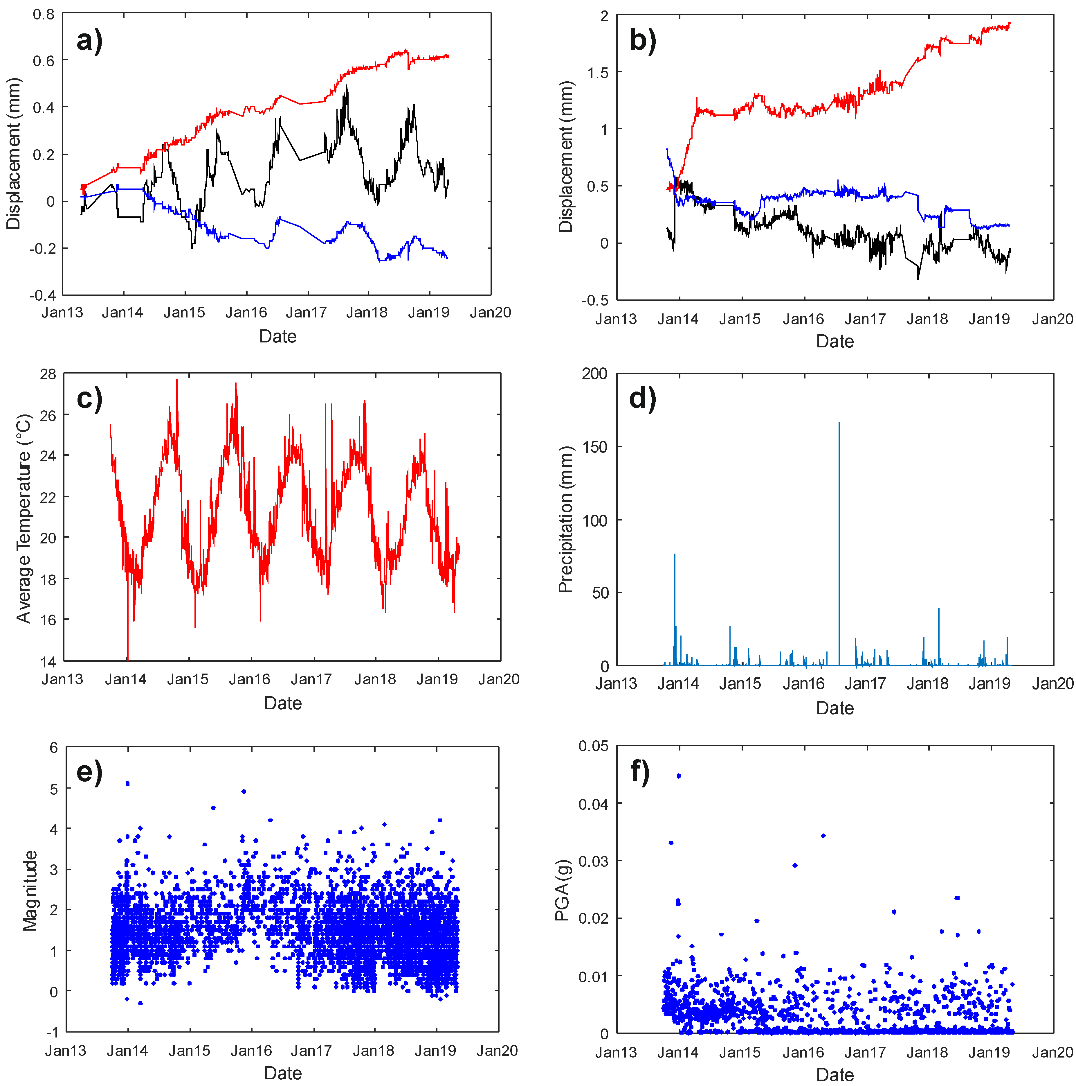
The data used in this analysis can be split into three categories: (i) data from the 3D dilatometers placed on the SAL detachment plane; (ii) climatic variables and (iii) seismicity (Figure 2).
3.1. 3D Dilatometer Data
Two 3D dilatometers named HIE2 and HIE3 are placed on the SAL’s detachment plane. They are about 2.5 km apart (Figure 1) and the measurements are taken every 24 h at 00:00 UTC. The records (Figure 2) are analyzed in a Cartesian coordinate system with X-axis showing compression/extension perpendicular to the detachment plane; Y-axis showing strike-slip movement along the detachment plane and Z-axis showing vertical movement perpendicular to the detachment plane. As the records are taken at 00:00 UTC the records were correlated with climatic and geophysical variables from the previous day. Automated monitoring started on 16/10/2013 and covers a period of 2010 d till 17/04/2019. Due to technical difficulties, several instrument failures resulting in missing records happened. In the case of HIE2 device, there are 494 missing measurements (24.6%), in the case of HIE3 there are 358 missing records (17.8%).
3.2. Climatic Variables
Climatic variables are strongly influencing any landslide behavior. For that purpose, temperature, precipitation and insolation data from the El Hierro airport [52] were downloaded. The location of this station is not directly on the SAL. However, it is in its vicinity and provides daily undisturbed data for the whole monitoring period. Precipitation can play a principal role in landslide activation. For that purpose, the daily rainfall amounts were analyzed. Additionally, the 30-day antecedent precipitation index (API30) [53,54] was calculated to better depict the influence of retrospective precipitation history and its influence on soil moisture [55]:
where n is the number of antecedent days; c is decay constant and it depends on watershed and seasonal parameters. The value of c ranges between 0.80 and 0.98 [56]. In this study, a c of 0.95 was used; i is the number of days counting backwards from the date on which the API is determined and Pn is the amount of precipitation i days before the causal rainfall (mm).
Mean and maximum daily temperatures can influence both the monitoring instrument and the rock on which it is attached by thermal dilation [57]. For that purpose, the temperature data were used to observe influence on the monitoring records and assess seasonal trends.
3.3. Seismic Data
Seismicity plays a major role in the stability of volcanic flanks. During the analyzed period, a total of 6537 seismic events were recorded around El Hierro Island by the Instituto Geográfico Nacional network [58]. We used this data to calculate the PGAs (Peak Ground Accelerations) of these events. The Canary Islands does not have developed local ground-motion attenuation relationship and there are no accelerometer network data available. For that reason, we applied an attenuation relationship developed for the Hawaiian Islands (to some point, a similar volcanic archipelago) by [59] and suggested to be used on the Canary Islands by [60]:
where PGA is measured in units of g, M is the magnitude, r = (d2 + 11.292)1/2 and S is 0 for lava sites and 1 at ash sites. The distance parameter d is the closest distance from the recording site to the surface projection of the fault rupture area.
For this analysis, we used the maximum recorded PGA for the particular day and also calculated the sums of daily PGAs (named PGA dose). The maximum PGAs and PGA doses were calculated for both HIE2 and HIE3 instruments considering their geographic location.
4. Methodological Approach
4.1. Input Data Pre-Processing
The relative motion on the detachment planes of the SAL is represented by time series which are not completely homogeneous. There are many missing values due to technical problems. This is not necessarily a problem as the reading frequency of the device (every 24 h) to the speed of the movement is very high. However, the methodology of time-series processing needs to be adapted to this fact.
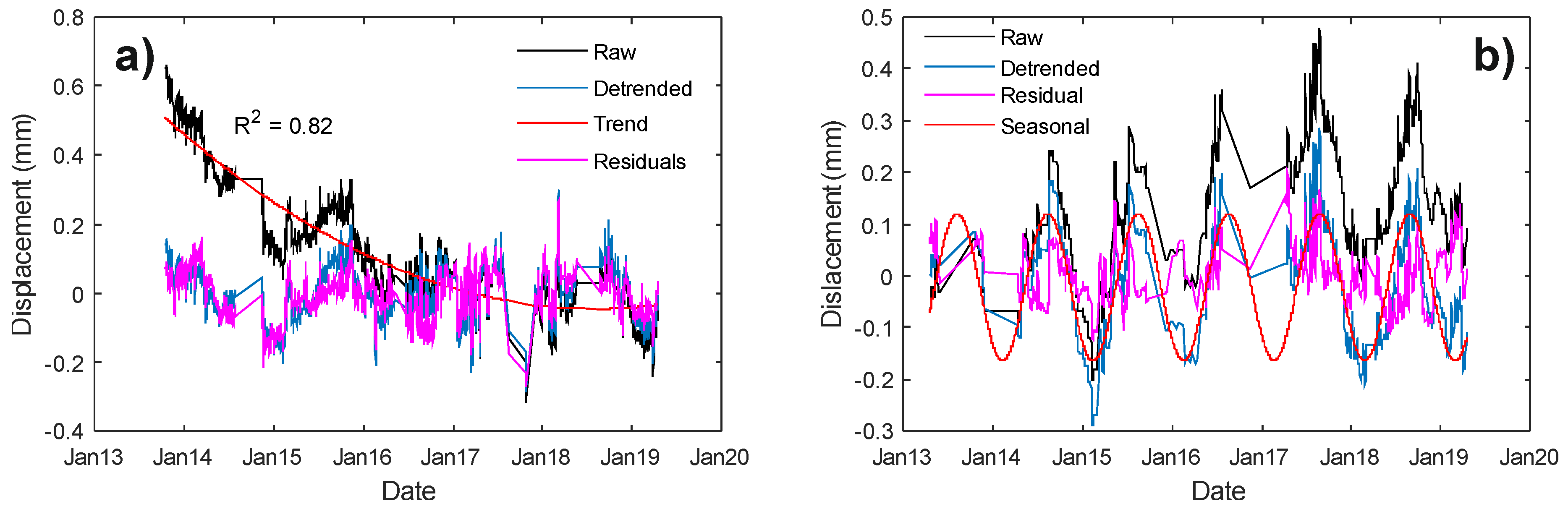
The time series were decomposed into trend, residual and seasonal components (as is visible on Figure 3). The periodicity of the seasonal components reflects the effect of the thermal dilation of the anchoring elements holding the TM-71 device, but it can also be partially influenced by the volume changes of the monitored blocks. A Fourier model was fitted to estimate the characteristics of the periodic component, specifically the 1st harmonics. The period of the harmonic function was fixed at 365 d (Figure 3b). The applicability of the harmonic function 0.15 mm corresponds to the amplitude of the air temperature (4 °C) and the length of the steel anchoring elements (2 m) at the coefficient of thermal expansion α = 16.3 × 10⁻⁶.
The trend component is very well described by the approximation by a second-order polynomial. This indicates a linear change in velocity over time. This trend is clearly visible on the HIE3 X-axis (Figure 3).
4.2. Detection of Change-Points in Time Series of Individual Components
The time series of the measured movements are not stationary but often express sudden changes. We assume that these changes are caused by external factors. Over time, several methods have been developed to detect such changes such as CUSUM (Cumulative Sum) and its modifications (firstly introduced by [61]). Limiting factors of a wide range of methods are very often the computational demands in combination with a large volume of data or the requirement for time-series homogeneity. The problem of geotechnical measurements (field measurements in general) is the incompleteness of the time series or its inhomogeneity—different time spacing between recorded measurements. In this work, the PARCS (Paired Adaptive Regressors for Cumulative Sum) method was used, a method for detecting a change in the mean value of the multidimensional time series [20]. The time series of measurements are burdened with random errors. The mean value is then close to the value of the monitored variable in a large number of measurements.
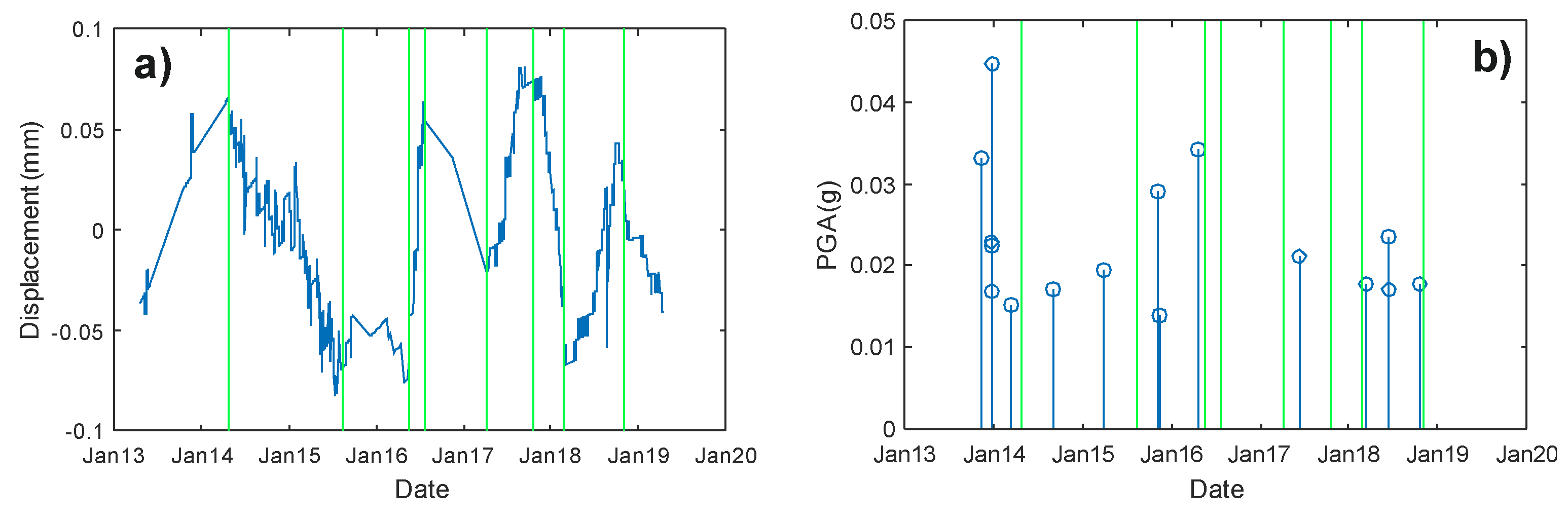
The PARCS method looks for a predefined number of change-points in the time series. The input data to the algorithm are an array containing the time-series data and the scalar value indicating the number of searched change-points (N). The advantage over other methods is that the time series may not be completely consistent and may contain holes. The PARCS method was modified for data analysis so that the input parameter N was used only as an a priori (initial) value and the target mean error parameter was added. After the detection of change-points, the time series is divided into segments, which are approximated by linear regression. If the standard deviation on one of the sections exceeds the given limit value, the parameter N is increased (Figure 4).
The cut-off target value of the standard deviation was derived from the assumed accuracy of the dilatometer measurement as twice the standard deviation of the measurement found during laboratory testing [62].
A relatively large number of change-points was detected. Taking a closer look at the trajectory of motion, it is clear that some of these change-points do not lead to a change in the trajectory of motion but are the result of chaotical behavior. Therefore, we decided to directly analyze the trajectory of motion in the plane (2D) and space (3D) to find the key points of its change and their time stamps (Figure 5).
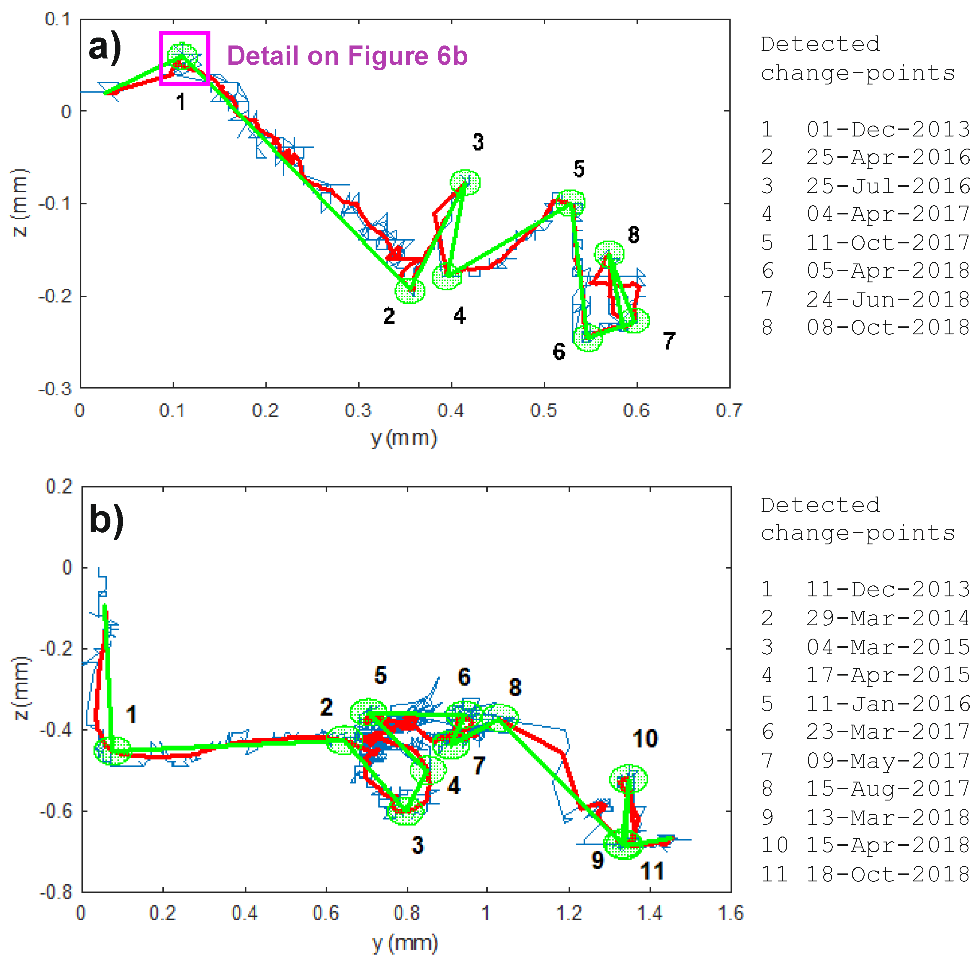
The trajectory of the movement is represented by an array of coordinates with a removed periodic component. At first, the trajectory was smoothed using a 30-day moving average of the position to remove random noise. Then, the key breaking points of the motion curve were found, the curve was expressed by the minimum number of linear segments so that the accuracy criterion was preserved (Figure 5). For this purpose, the Ramer–Douglas–Peuckner (RDP) simplification algorithm was used [63]. The advantage of this approach is that all three components of motion can be analyzed together. Compared to other change-point detection methods applied to components, the RDP algorithm is simpler and enables very fast sampling of the curve and detection of change-points.
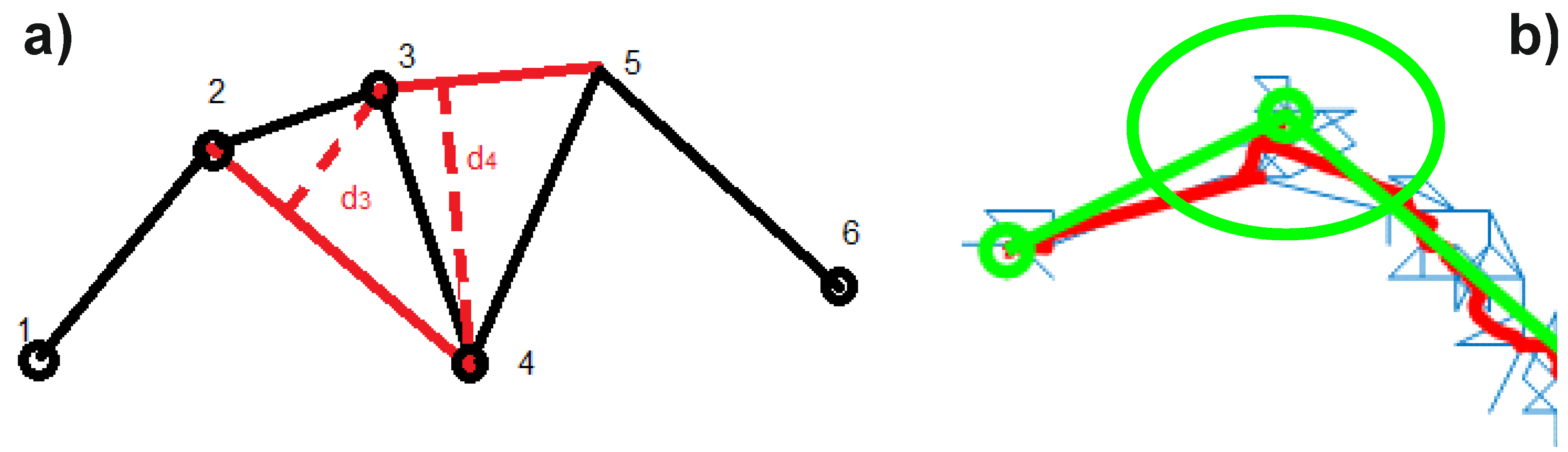
Importance of the change-points was rated to highlight the most significant changes in the pathway of movement of the monitored SAL detachment plane. We assume that the importance of change-point is increasing with its shortest distance from the connection of two adjacent change-points (Figure 6). The most significant changes in the trajectories were highlighted by red stars (Figures 10 and 11).
Note that in the figure above (Figure 6b), the change-point is displayed as one single moment, but a closer view to the trajectory of the movement shows, that in case of such slow movement (daily displacement is smaller than random noise) there should be some temporal buffer around the change-point where the trajectory is changing. This enabled to decide if the change of the trajectory is the reaction on a given event (for example seismic).
The time span of possible change-point location is in two- or three-dimensional space represented by error ellipse or ellipsoid, where its center is located in the change-point. The size of the major and minor axes of the ellipse/ellipsoid is derived from the magnitude of the standard deviations in the respective directions. All points of the trajectory located within the ellipse/ellipsoid are detected as possible change-points, and, therefore, each turn of the trajectory is represented by a set of relevant time stamps. As a consequence, one turn of the trajectory is now represented with various numbers of dates, which can be confronted with the time stamps of other events.
Both approaches: change-point detection in time series of components and trajectory simplification leads to detecting time stamps, which were then confronted with time stamps of above normal events in the time series of potential landslide triggers.
We assume that significant events in the movement are caused by significant events in the seismicity or precipitation. Statistics describe this relation as causality. We used Granger causality to quantify the relationship between sets of events with different extents, which allows determining if one set of values is caused by another on a given significance level [64].
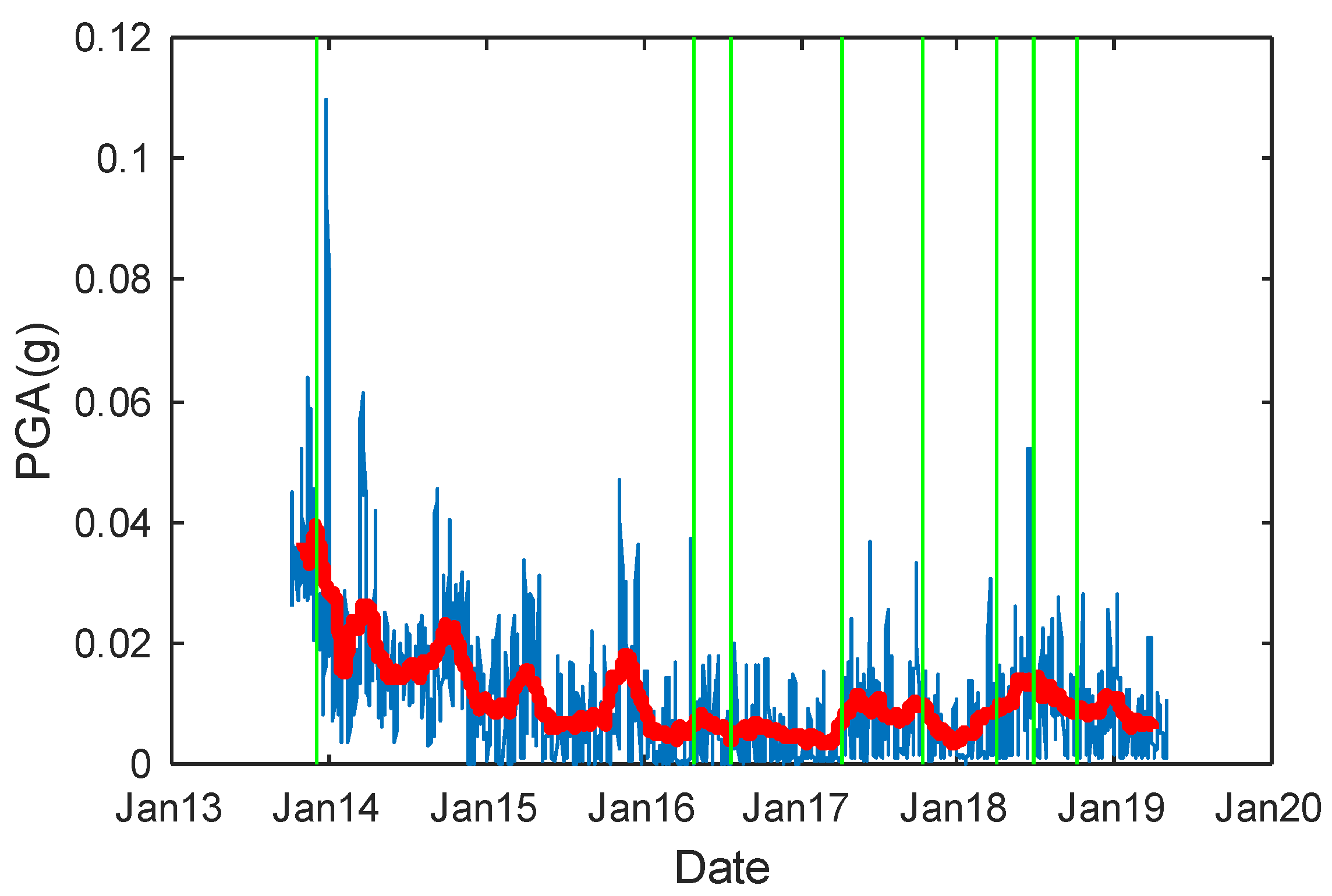
There was a huge number of seismic events during the analyzed period—most of them with very low magnitude. To compare seismic events with significant events in the movement, it was needed to highlight above normal seismic events. For this reason, the average value and standard deviation of daily PGA maxima were computed. Then, only those seismic events were selected whose standard deviation of maximum PGA average was three times higher than the standard deviation. To highlight episodes with higher seismicity, five-day sums of PGA maxima were computed (Figure 7).
5. Results and Discussion
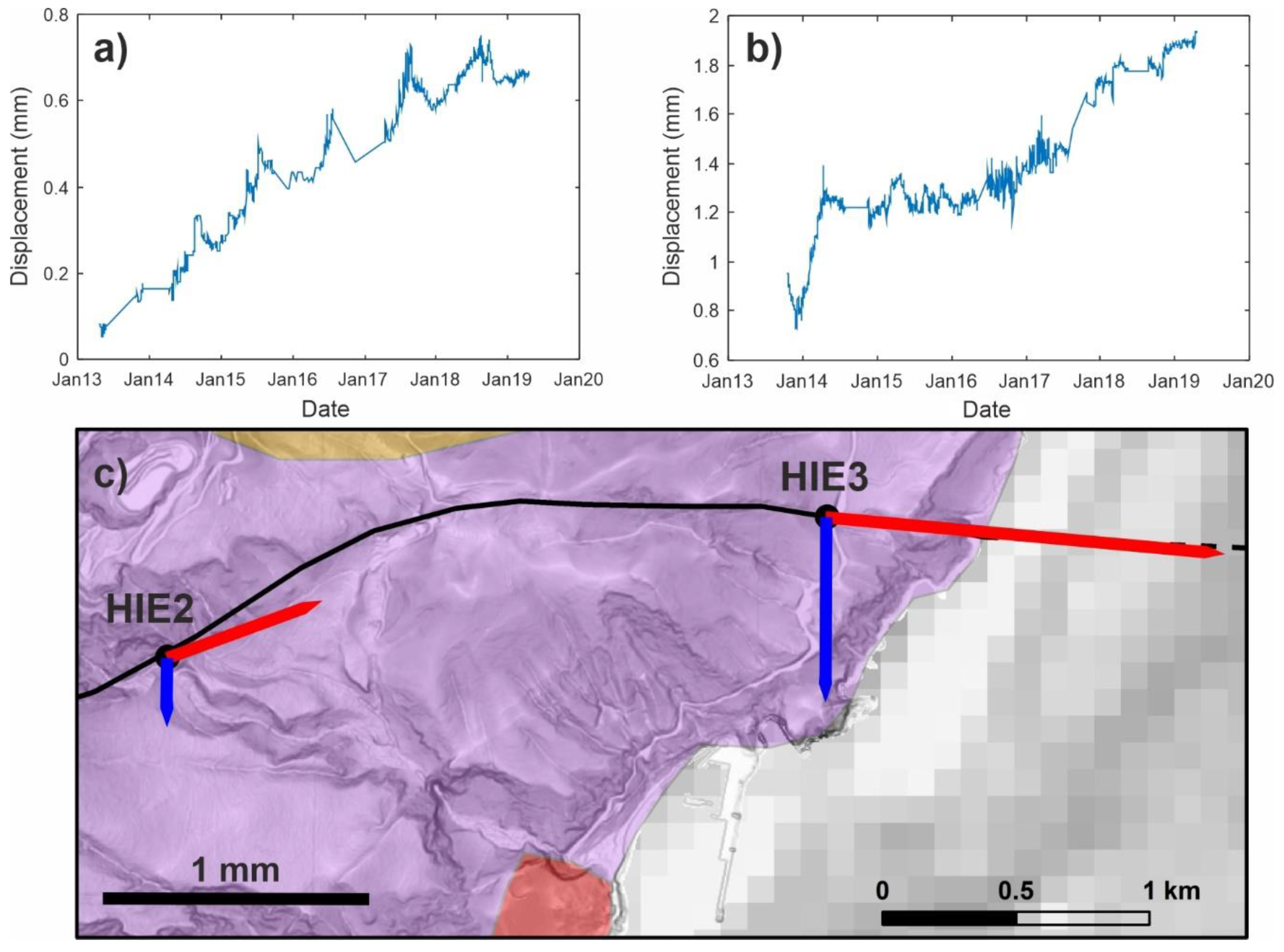
Figure 8 shows the total displacement distance from the beginning of the monitoring. There is a visible decrease in movement speed on both devices. Although, in the case of HIE3 this is less pronounced.
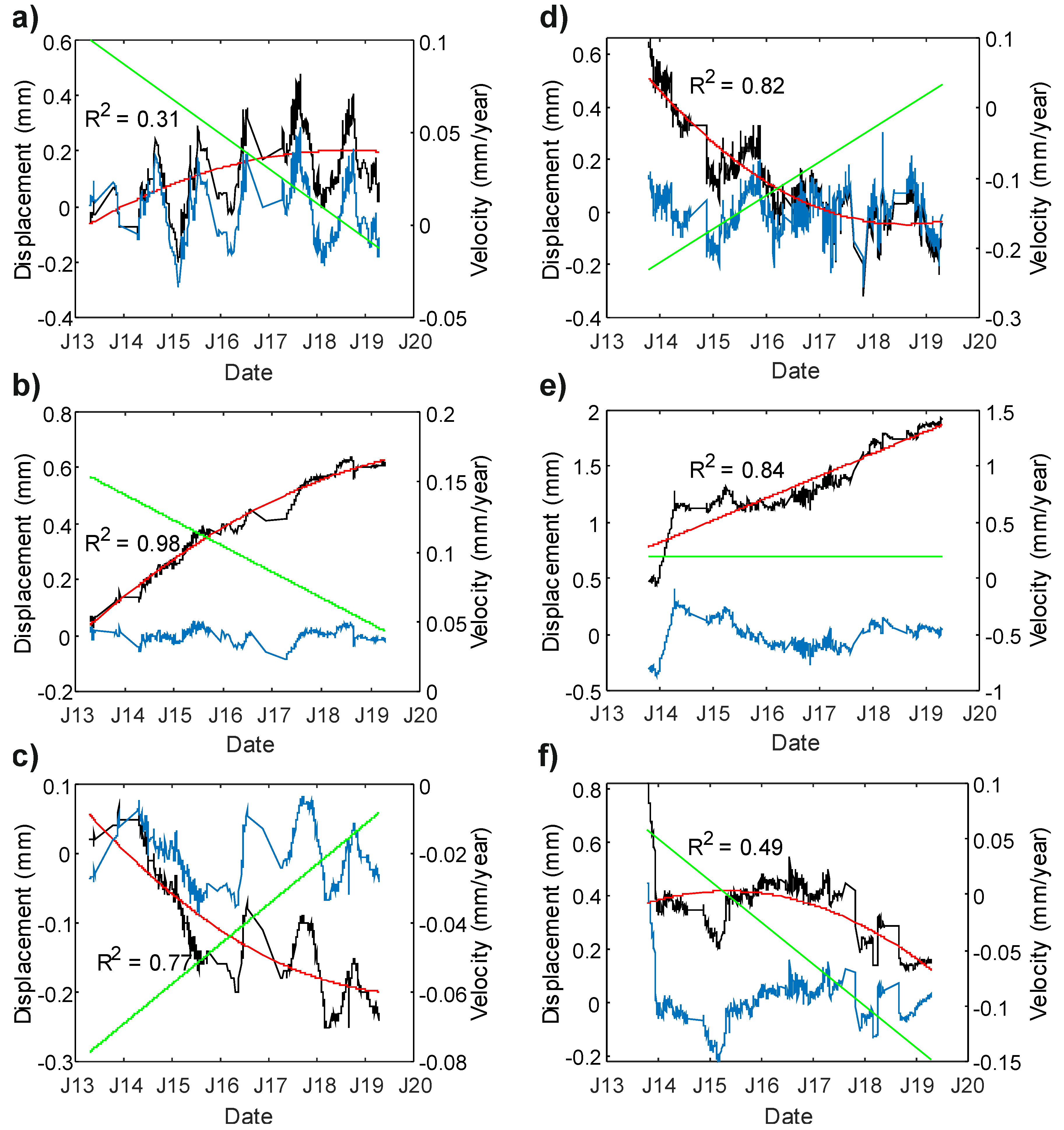
Both 3D dilatometers HIE2 and HIE3 showed permanent very slow creep movement during the analyzed period, generally in the downslope sense. It can be noted from Figure 8c, that on HIE3 device the horizontal component of the movement is parallel to the general slope. On HIE2 device the horizontal component of the movement is almost perpendicular to the general slope (sinistral strike slip). This is probably a long-term behavior, which was already documented by [47] and it is recognizable on a step-like shape of the gully below the device. On both dilatometric devices the movement direction corresponds to the El Hierro earthquake and volcanic activity epicenters, which are concentrated to the west and southwest from the SAL landslide. The speed of the movement and its direction changed over time. Movement trend on the HIE2 device is well described by a second order polynomial (Figure 9a–c). The X and Y axes show a close-to-linear decrease in the speed of the movement.
Analysis of GNSS and InSAR data from the beginning of the 3D dilatometer monitoring period [29] shows large absolute movements of the island in the period from July 2012 to March 2014. Although there are no permanent GNSS receivers on the SAL body, the nearest permanent GNSS stations show northeast shift and uplift of several centimeters. Similar results are shown from InSAR data, which are available for the island. The results, however, show largest surface movements in the western and southwestern parts of the island, while the SAL body on the northeast was much more stable at that time. It has to be noted, however, that HIE2 and HIE3 automatic devices are measuring relative movements on the detachment plane, while GNSS and InSAR are showing absolute movements of the island.
PS InSAR analysis performed for the period from October 2013 to October 2015 [65] shows rather different behavior on different parts of the SAL body, suggesting that the landslide moves as separate creeping blocks (as also shown in [32]). The speed of the movement during the two-year analyzed period reaches few mm.a−1 downslope.
It has to be noted that a principal road connecting the La Estaca port with the island’s capital Valverde is crossing the SAL detachment plane just below the HIE3 dilatometer. This road has been damaged by cracks during 2012–2014 with general direction along the detachment plane, and the tarmac had to be repaired.
Movement trends on the HIE3 device are much more fluctuating (Figure 9d–f). This is not surprising considering the fact, that this device is installed in the open air and thus more prone to climatic influence (i.e., temperature changes, humidity). In the case of the Z-axis, the movement speed seems to slightly increase. This is most probably due to the fact, that this device is measuring a separated block within the entire landslide body, which exhibits slightly different behavior than the rest of the landslide [32].
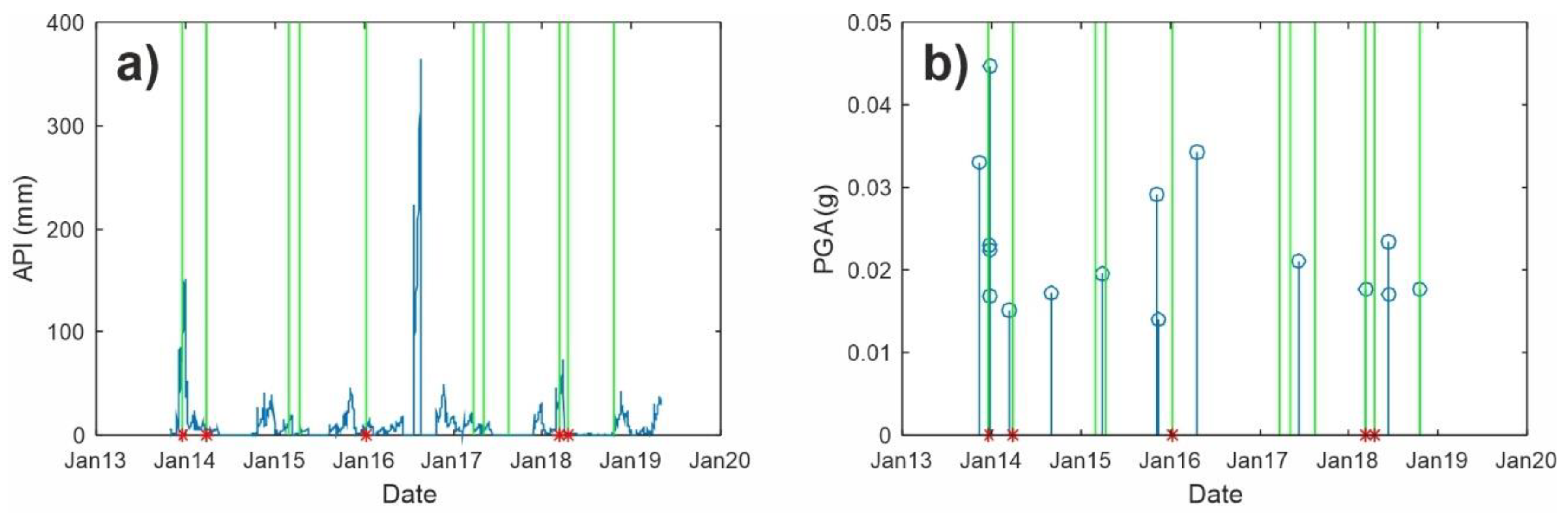
It can be seen, that most significant changes in the direction of the movement happened in December 2013, at the very beginning of the monitoring. Comparison of the change-points in the trajectory on both HIE2 and HIE3 with the PGA and API are shown on Figure 10 and Figure 11. There is a recognizable correlation of seismic activity and changes of movements on both devices. However, HIE2 shows more movement changes correlating with PGA than the HIE3 device. The most notable change-point probably influenced by the seismic activity occurred at the end of December 2013, when the strongest earthquake during the monitoring period (M = 5.1) also occurred. Other change-points presumably influenced by seismic activity happened in 14-Nov-2013; 23-Dec-2013; 24-Dec-2013; 25-Dec-2013; 28-Dec-2013; 16-Mar-2014; 04-Sep-2014; 30-Mar-2015; 08-Nov-2015; 13-Nov-2015; 21-Apr-2016; 08-Jun-2017; 14-Mar-2018; 14-Jun-2018; 15-Jun-2018 and 17-Oct-2018.
In case of API there is not a clearly visible correlation with change-points, except in December 2013; July 2016 and April 2018 affecting the HIE3 device and July 2016 affecting the HIE2 device. This suggests that the nature of the measured movement has, more probably, an endogenous cause. These observed results are in good accordance with the analysis performed by [32]. In their study, a period from October 2013 to June 2014 was analyzed on the HIE3 device. Three major impulses were recognized (rainfall event in December 2013 and seismic events in December 2013 and March 2014). All these three impulses were also identified using this proposed methodology.
However, during most of the analyzed period, there is no clear correlation between change-points and seismic or rainfall activity. This can be caused by two reasons. Firstly, the seismic activity (PGA), which is presumed to be the main triggering factor of SAL movement [49], has ceased significantly since 2013, as is decreasing the average speed of movement of the SAL documented in this work; changes in the residuals are negligible. Secondly, the influence of precipitation (API) is probably negligible on the SAL behavior. Only three events were identified, mostly affecting the HIE3 device. This is probably caused by the presence of a shallower landslide block influenced by precipitation (see [32] for more details).
6. Conclusions
The proposed methodology allowed us to process a large amount of monitoring non-stationary data and to find critical time stamps—change-points, when the nature of the monitored landslide movement changed significantly. Moreover, it suppresses the influence of the scientist, who is always subjective and to some point tends to find what he is looking for.
The PARCS method detects change-points very well but is relatively hardware-demanding. It has to be noted, however, that the magnitude of the detected changes is close to the confidence limit of the measurements determined in laboratory conditions [62]. It is worth noting the significant change in the trajectory of motion detected on both measuring devices in December 2013 was influenced by both precipitation (at the beginning of December) and strong seismicity (24–26 December).
Despite not acquiring unambiguous results in terms of the geological interpretation, we believe that the proposed methodological approach can significantly contribute to the landslide monitoring data analysis of any slow-moving landslides in the future by both:
- (i)
- decreasing the subjectivity of interpretation and
- (ii)
- allowing fully quantitative analysis of the monitored data of a slow-moving landslide.
Future research should focus more on defining the influencing magnitude of the triggering factors to determine better the behavior of the SAL in the future.
Author Contributions
Conceptualization, J.B. (Jan Blahůt) and J.B. (Jan Balek); methodology, J.B. (Jan Blahůt) and J.B. (Jan Balek); formal analysis, J.B. (Jan Balek) and M.E.; investigation, J.B. (Jan Blahůt), S.M.; data curation, J.B. (Jan Blahůt), J.B. (Jan Balek) and M.A., writing—original draft preparation, J.B. (Jan Blahůt), J.B. (Jan Balek); visualization, J.B. (Jan Blahůt), J.B. (Jan Balek), writing—revision, J.B. (Jan Blahůt), J.B. (Jan Balek). All authors have read and agreed to the published version of the manuscript.
Funding
This research was funded by the Czech Science Foundation, grant number GJ16-12227Y and by the long-term conceptual development research organization RVO: 67985891.
Acknowledgments
The authors are indebted to María José Blanco and her staff at the Centro Geofísico de Canarias (IGN) for their help with installation and maintenance of the 3D dilatometer monitoring points on El Hierro and IGN for the open seismic data availability. OGIMET is acknowledged for providing daily meteorological data from the El Hierro Airport. Jana Šreinová and Monika Hladká are thanked for processing and analyzing the 3D dilatometer data. We also thank to the two anonymous reviewers who helped to improve the clarity of the manuscript.
Conflicts of Interest
The authors declare no conflict of interest. The funders had no role in the design of the study; in the collection, analyses or interpretation of data; in the writing of the manuscript, or in the decision to publish the results.
References
- Corominas, J.; Moya, J.; Ledesma, A.; Lloret, A.; Gill, J.A. Prediction of ground displacements and velocities from groundwater level changes at the Vallcebre Landslide (Eastern Pyrenees, Spain). Landslides 2005, 2, 83–96. [Google Scholar] [CrossRef]
- Van Asch, T.W.J.; Van Beek, L.P.H.; Bogaard, T.A. Problems in predicting the mobility of slow-moving landslides. Eng. Geol. 2007, 91, 46–55. [Google Scholar] [CrossRef]
- Klimeš, J.; Rowberry, M.; Blahůt, J.; Briestenský, M.; Hartvich, F.; Košťák, B.; Rybář, J.; Stemberk, J.; Štěpančíková, P. The monitoring of slow-moving landslides and assessment of stabilisation measures using an optical–mechanical crack gauge. Landslides 2012, 9, 407–415. [Google Scholar] [CrossRef]
- Carey, J.M.; Massey, C.I.; Lyndsell, B.; Petley, D.N. Displacement mechanisms of slow-moving landslides in response to changes in porewater pressure and dynamic stress. Earth Surf. Dynam. 2019, 7, 707–722. [Google Scholar] [CrossRef] [Green Version]
- Singh, L.P.; Van Westen, C.J.; Champati Ray, P.K.; Pasquali, P. Accuracy assessment of InSAR derived input maps for landslide susceptibility analysis: A case study from the Swiss Alps. Landslides 2005, 2, 221–228. [Google Scholar] [CrossRef]
- Schmidt, K.; Reimann, J.; Tous Ramon, N.; Schwerdt, M. Geometric accuracy of Sentinel-1A and 1B derived from SAR raw data with GPS surveyed corner reflector positions. Remote Sens. 2018, 10, 523. [Google Scholar] [CrossRef] [Green Version]
- Sinharay, S. An Overview of Statistics in Education. In International Encyclopedia of Education, 3rd ed.; Peterson, P., Baker, E., McGaw, B., Eds.; Elsevier: Amsterdam, The Netherlands, 2010; pp. 1–11. [Google Scholar] [CrossRef]
- Brillinger, D.R. Time Series: General. In International Encyclopedia of the Social & Behavioral Sciences, 1st ed.; Smelser, N.J., Baltes, P.B., Eds.; Elsevier: Amsterdam, The Netherlands, 2001; pp. 15724–15731. [Google Scholar] [CrossRef]
- Lütkepohl, H. New Introduction to Multiple Time Series Analysis; Springer: Heidelberg, Germany, 2005; p. 764. [Google Scholar]
- Neusser, K. Time Series Econometrics; Springer: Heidelberg, Germany, 2016; p. 409. [Google Scholar] [CrossRef]
- Montillet, J.-P.; Bos, M.S. Geodetic Time Series Analysis in Earth Sciences; Springer: Heidelberg, Germany, 2020; p. 422. [Google Scholar] [CrossRef]
- Mudelsee, M. Climate Time Series Analysis; Springer: Heidelberg, Germany, 2014; p. 454. [Google Scholar] [CrossRef]
- Sun, L.; Muller, J.-P.; Chen, J. Time series analysis of very slow landslides in the Three Gorges Region through small baseline SAR offset tracking. Remote Sens. 2017, 9, 1314. [Google Scholar] [CrossRef] [Green Version]
- Pfeiffer, J.; Zieher, T.; Rutzinger, M.; Bremer, M.; Wichmann, V. Comparison and time series analysis of landslide displacement mapped by airborne, terrestrial and unmanned aerial vehicle based platforms. ISPRS Ann. Photogramm. Remote Sens. Spat. Inf. Sci. 2019, IV-2/W5, 421–428. [Google Scholar] [CrossRef] [Green Version]
- Huang Lin, C.; Liu, D.; Liu, G. Landslide detection in La Paz City (Bolivia) based on time series analysis of InSAR data. Int. J. Remote Sens. 2019, 40, 6775–6795. [Google Scholar] [CrossRef]
- Zvelebil, J.; Stemberk, J. Slope monitoring applied to rock fall management in NW Bohemia. In Landslide Research, Theory and Practice: Proceedings of the 8th International Symposium on Landslides held in Cardiff on 26–30 June 2000; Broomhead, E., Ed.; Thomas-Telford: London, UK, 2000; Volume 3, pp. 1659–1664. [Google Scholar]
- Košťák, B. Deformation effects in rock massifs and their long-term monitoring. Q. J. Eng. Geol. Hydrogeol. 2006, 39, 249–258. [Google Scholar] [CrossRef]
- Nikolakopoulos, K.; Kavoura, K.; Depountis, N.; Kyriou, A.; Argyropoulos, N.; Koukouvelas, I.; Sabatakakis, N. Preliminary results from active landslide monitoring using multidisciplinary surveys. Eur. J. Remote Sens. 2017, 50, 280–299. [Google Scholar] [CrossRef] [Green Version]
- Guignard, F.; Laib, M.; Amato, F.; Kanevski, M. Advanced analysis of temporal data using Fisher-Shannon Information: Theoretical development and application in Geosciences. Fron. Earth Sci. 2020, 8, 255. [Google Scholar] [CrossRef]
- Toutounji, H.; Durstewitz, D. Detecting multiple change points using adaptive regression splines with application to neural recordings. Front. Neuroinform. 2018, 12, 67. [Google Scholar] [CrossRef] [PubMed] [Green Version]
- Alippi, C.; Camplani, R.; Galperti, C.; Marullo, A.; Roveri, M. An hybrid wireless-wired monitoring system for real-time rock collapse forecasting. In Proceedings of the 7th International Conference on Mobile Ad hoc and Sensor System (MASS), San Francisco, CA, USA, 8–12 November 2010; pp. 224–231. [Google Scholar]
- Barile, G.; Leoni, A.; Pantoli, L.; Stornelli, V. Real-Time Autonomous System for Structural and Environmental Monitoring of Dynamic Events. Electronics 2018, 7, 420. [Google Scholar] [CrossRef] [Green Version]
- Tordesillas, A.; Zhou, Z.; Batterham, R. A data-driven complex systems approach to early prediction of landslides. Mech. Res. Commun. 2018, 92, 137–141. [Google Scholar] [CrossRef]
- Bontemps, N.; Lacroix, P.; Larose, E.; Jara, J.; Taipe, E. Rain and small earthquakes maintain a slow-moving landslide in a persistent critical state. Nat. Commun. 2020, 11, 780. [Google Scholar] [CrossRef]
- Guillou, H.; Carracedo, J.-C.; Pérez Torrado, F.; Rodríguez Badiola, E. K-Ar ages and magnetic stratigraphy of a hotspot-induced, fast grown oceanic island: El Hierro, Canary Islands. J. Volcanol. Geotherm. Res. 1996, 73, 141–155. [Google Scholar] [CrossRef]
- Becerril, L.; Ubide, T.; Sudo, M.; Martí, J.; Galindo, I.; Galé, C.; Morales, J.; Yepes, J.; Lago, M. Geochronological constraints on the evolution of El Hierro (Canary Islands). J. Afr. Earth Sci. 2016, 113, 88–94. [Google Scholar] [CrossRef]
- Carracedo, J.-C.; Rodríguez Badiola, E.; Guillou, H.; de la Nuez, H.; Pérez Torrado, F. Geology and volcanology of the western Canaries: La Palma and El Hierro. Estudios Geológicos 2001, 57, 171–295. [Google Scholar] [CrossRef] [Green Version]
- López, C.; Blanco, M.J.; Abella, R.; Brenes, B.; Cabrera Rodríguez, V.; Casas, B.; Domínguez Cerdeña, I.; Felpeto, A.; Fernández de Villalta, M.; del Fresno, C.; et al. Monitoring the volcanic unrest of El Hierro (Canary Islands) before the onset of the 2011–2012 submarine eruption. Geophys. Res. Lett. 2012, 39, L13303. [Google Scholar] [CrossRef]
- Benito-Saz, M.; Parks, M.; Sigmundsson, F.; Hooper, A.; García-Cañada, L. Repeated magmatic intrusions at El Hierro Island following the 2011–2012 submarine eruption. J. Volcanol. Geotherm. Res. 2017, 344, 79–91. [Google Scholar] [CrossRef] [Green Version]
- Meletlidis, S.; Di Roberto, A.; Domínguez Cerdeña, I.; Pompilio, M.; García-Cañada, L.; Bertagnini, A.; Benito-Saz, M.; Del Carlo, P.; Sainz-Maza Aparicio, S. New insight into the 2011–2012 unrest and eruption of El Hierro Island (Canary Islands) based on integrated geophysical, geodetical, and petrological data. Ann. Geophys. 2015, 58, S0546. [Google Scholar] [CrossRef]
- Carracedo, J.-C.; Troll, V. The Geology of Canary Islands, 1st ed.; Elsevier: Amsterdam, The Netherlands, 2016; p. 622. [Google Scholar]
- Blahůt, J.; Baroň, I.; Sokol, Ľ.; Meletlidis, S.; Klimeš, J.; Rowberry, M.; Melichar, R.; García-Cañada, L.; Martí, X. Large landslide stress states calculated during extreme climatic and tectonic events on El Hierro, Canary Islands. Landslides 2018, 15, 1801–1814. [Google Scholar] [CrossRef]
- Masson, D. Catastrophic collapse of the volcanic island of Hierro 15 ka ago and the history of landslides in the Canary Islands. Geology 1996, 24, 231–234. [Google Scholar] [CrossRef]
- Urgeles, R.; Canals, M.; Baraza, J.; Alonso, B. The submarine El Golfo debris avalanche and the Canary debris flow, west Hierro Island: The last major slides in the Canary Archipelago. Geogaceta 1996, 20, 390–393. [Google Scholar]
- Urgeles, R.; Canals, M.; Baraza, J.; Alonso, B.; Masson, D. The most recent megalandslides on the Canary Islands: The El Golfo debris avalanche and the Canary debris flow, west El Hierro Island. J. Geophys. Res. Solid Earth 1997, 102, 20305–20323. [Google Scholar] [CrossRef]
- Carracedo, J.-C.; Day, S.; Guillou, H.; Pérez Torrado, F. Giant quaternary landslides in the evolution of La Palma and El Hierro, Canary Islands. J. Volcanol. Geotherm. Res. 1999, 94, 169–190. [Google Scholar] [CrossRef]
- Masson, D.; Watts, A.B.; Gee, M.J.; Urgeles, R.; Mitchell, N.; Le Bas, T.; Canals, M. Slope failures on the flanks of the western Canary Islands. Earth Sci. Rev. 2002, 57, 1–35. [Google Scholar] [CrossRef]
- Longpré, M.; Chadwick, J.; Wijbrans, J.; Iping, R. Age of the El Golfo debris avalanche, El Hierro (Canary Islands): New constraints from laser and furnace 40Ar/39Ar dating. J. Volcanol. Geotherm. Res. 2011, 203, 76–80. [Google Scholar] [CrossRef]
- Becerril, L.; Galve, J.; Morales, J.; Romero, C.; Sánchez, N.; Martí, J.; Galindo, I. Volcanostructure of El Hierro (Canary Islands). J. Maps 2016, 12, 43–52. [Google Scholar] [CrossRef] [Green Version]
- León, R.; Somoza, L.; Urgeles, R.; Medialdea, T.; Ferrer, M.; Biain, A.; García-Crespo, J.; Mediato, J.; Galindo, I.; Yepes, J.; et al. Multi-event oceanic island landslides: New onshore-offshore insights from El Hierro Island, Canary archipelago. Mar. Geol. 2017, 393, 156–175. [Google Scholar] [CrossRef]
- Blahůt, J.; Klimeš, J.; Rowberry, M.; Kusák, M. Database of giant landslides on volcanic islands—First results from the Atlantic Ocean. Landslides 2018, 15, 823–827. [Google Scholar] [CrossRef]
- Blahůt, J.; Balek, J.; Klimeš, J.; Rowberry, M.; Kusák, M.; Kalina, J. A comprehensive global database of giant landslides on volcanic islands. Landslides 2019, 16, 2045–2052. [Google Scholar] [CrossRef]
- Agliardi, F.; Crosta, G.; Zanchi, A. Structural constraints on deep seated slope deformation kinematics. Eng. Geol. 2001, 59, 83–102. [Google Scholar] [CrossRef]
- Moscardelli, L.; Wood, L. New classification system for mass transport complexes in offshore Trinidad. Basin Res. 2008, 20, 73–98. [Google Scholar] [CrossRef]
- Day, S.; Carracedo, J.-C.; Guillou, H. Age and geometry of an aborted rift flank collapse: The San Andres fault system, El Hierro, Canary Islands. Geol. Mag. 1997, 134, 523–537. [Google Scholar] [CrossRef]
- Blahůt, J.; Mitrovic-Woodell, I.; Baroň, I.; René, M.; Rowberry, M.; Blard, P.-H.; Hartvich, F.; Balek, J.; Meletlidis, S. Volcanic edifice slip events recorded on the fault plane of the San Andrés Landslide, El Hierro, Canary Islands. Tectonophysics 2020, 776, 228317. [Google Scholar] [CrossRef]
- Klimeš, J.; Yepes, J.; Becerril, L.; Kusák, M.; Galindo, I.; Blahůt, J. Development and recent activity of the San Andrés Landslide on El Hierro, Canary Islands, Spain. Geomorphology 2016, 261, 119–131. [Google Scholar] [CrossRef] [Green Version]
- Blahůt, J.; Rowberry, M.; Balek, J.; Klimeš, J.; Baroň, I.; Meletlidis, S.; Martí, X. Monitoring giant landslide detachment planes in the era of big data analytics. In Advancing Culture of Living with Landslides; Mikoš, M., Arbanas, Ž., Yin, Y., Sassa, K., Eds.; Springer: Cham, Switzerland, 2017; Volume 3, pp. 333–340. [Google Scholar] [CrossRef]
- Blahůt, J.; Olejár, F.; Rott, J.; Petružálek, M. Current stability modelling of an incipient San Andrés giant landslide on El Hierro Island, Canaries, Spain—First attempt using limited input data. Acta Geodyn. Geomater. 2020, 17, 89–99. [Google Scholar] [CrossRef]
- Martí, X.; Rowberry, M.D.; Blahůt, J. A MATLAB® code for counting the moiré fringe patterns recorded on the optical-mechanical crack gauge TM-71. Comput. Geosci. 2013, 52, 164–167. [Google Scholar] [CrossRef]
- Stemberk, J.; Briestenský, M.; Cacoń, S. The recognition of transient compressional fault slow-slip along the northern shore of Hornsund Fjord, SW Spitsbergen, Svalbard. Pol. Polar Res. 2015, 36, 109–123. [Google Scholar] [CrossRef]
- Weather Information Service. Available online: http://www.ogimet.com/index.phtml.en (accessed on 6 June 2019).
- Kohler, M.A.; Linsley, R.K., Jr. Predicting Runoff from Storm Rainfall, Research Paper 34; US Weather Bureau: Washington, DC, USA, 1951.
- Mishra, S.K.; Singh, V.P. Soil Conservation Service Number (SCS-CN) Methodology; Kluwer Academic Publisher: Dordrecht, The Netherlands, 2003; p. 516. [Google Scholar]
- Smolíková, J.; Blahůt, J.; Vilímek, V. Analysis of rainfall preceding debris flows on the Smědavská hora Mt., Jizerské hory Mts., Czech Republic. Landslides 2016, 13, 683–696. [Google Scholar] [CrossRef]
- Viessman, W.; Lewis, G.L. Introduction to Hydrology, 4th ed.; Harper Collins: New York, NY, USA, 1996; p. 760. [Google Scholar]
- Racek, O.; Blahůt, J.; Hartvich, F. Monitoring of thermoelastic wave within a rock mass coupling information from IR camera and crack meters: A 24-hour experiment on “Branická skála” Rock in Prague, Czechia. In WLF5 Book—Volume 3 “Monitoring and Early Warning”; Springer: Berlin/Heidelberg, Germany, 2019. [Google Scholar]
- Instituto Geográfico Nacional. Available online: https://www.ign.es/web/ign/portal/sis-catalogo-terremotos (accessed on 6 June 2019).
- Munson, C.G.; Thurber, C.H. Analysis of the attenuation of strong ground motion on the Island of Hawaii. Bull. Seismol. Soc. Am. 1997, 87, 945–960. [Google Scholar]
- Gonzáles de Vallejo, L.I.; García-Mayordomo, J.; Insua, J.M. Probabilistic seismic-hazard assessment of the Canary Islands. Bull. Seismol. Soc. Am. 2006, 96, 2040–2049. [Google Scholar] [CrossRef]
- Page, E.S. Continuous inspection schemes. Biometrika 1954, 41, 100–115. [Google Scholar] [CrossRef]
- Balek, J.; Urban, R.; Štroner, M. Laboratory testing of the precision and accuracy of the TM-71 dilatometer. Pap. SGEM 2018, 18, 433–439. [Google Scholar] [CrossRef]
- Visvalingam, M.; Whyatt, J.D. The Douglas-Peucker algorithm for line simplification: Re-evaluation through visualization. Comput. Graph. Forum 1990, 9, 213–228. [Google Scholar] [CrossRef]
- Granger, C.W.J. Investigating causal relations by econometric models and cross-spectral methods. Econometrica 1969, 37, 424–438. [Google Scholar] [CrossRef]
- Brasca Merlin, A.; Lanfri, M.; Carignano, C.; Pascual, I.; Schlögel, R.; Cuozzo, G. Sensado Remoto de procesos de remoción en masa: Pautas para el monitoreo operativo. In Proceedings of the 2018 IEEE Biennial Congress of Argentina (ARGENCON), San Miguel de Tucumán, Argentina, 6 June 2018; p. 8. [Google Scholar]
Figure 1.
Location of the study area: (a) the El Hierro Island with a simplified geological map showing the location of the TM-71 3D dilatometers and showing the direction of the axis (X, Y, Z) of the measurement: grey rectangle shows the location of Figure 8c; (b) dilatometer HIE2 located underground on the upper scarp of the SAL; (c) dilatometer HIE3 located in the open air on the left side of the SAL.

Figure 2.
Data used in the analysis: (a) HIE2 dilatometer: X-axis—black line, Y-axis—red line, Z-axis—blue line; (b) HIE3 dilatometer: X-axis—black line, Y-axis—red line, Z-axis—blue line; (c) daily average air temperatures; (d) daily precipitation; (e) registered earthquakes; (f) calculated PGA.
Figure 2.
Data used in the analysis: (a) HIE2 dilatometer: X-axis—black line, Y-axis—red line, Z-axis—blue line; (b) HIE3 dilatometer: X-axis—black line, Y-axis—red line, Z-axis—blue line; (c) daily average air temperatures; (d) daily precipitation; (e) registered earthquakes; (f) calculated PGA.

Figure 3.
Example of the time-series decomposition: (a) close to a linear decrease of the velocity on HIE3 Y-axis; (b) significant seasonal periodicity visible on HIE2 X-axis.
Figure 3.
Example of the time-series decomposition: (a) close to a linear decrease of the velocity on HIE3 Y-axis; (b) significant seasonal periodicity visible on HIE2 X-axis.

Figure 4.
Modified PARCS method applied to the time series of residual values (HIE3 z-axis): (a) time stamps of detected change-points marked in green, target standard deviation of 0.05 mm; (b) comparison of detected time stamps and seismic events.
Figure 4.
Modified PARCS method applied to the time series of residual values (HIE3 z-axis): (a) time stamps of detected change-points marked in green, target standard deviation of 0.05 mm; (b) comparison of detected time stamps and seismic events.

Figure 5.
Example of the processing of the movement trajectory on a Z-Y plane on: (a) HIE2 device; (b) HIE3 device: raw trajectory (blue), smoothed trajectory using 30-day moving average (red), simplified trajectory (green).
Figure 5.
Example of the processing of the movement trajectory on a Z-Y plane on: (a) HIE2 device; (b) HIE3 device: raw trajectory (blue), smoothed trajectory using 30-day moving average (red), simplified trajectory (green).

Figure 6.
(a) Importance of change-points was quantified using minimal distance di; (b) change-point defined using error ellipse.
Figure 6.
(a) Importance of change-points was quantified using minimal distance di; (b) change-point defined using error ellipse.

Figure 7.
Cumulated PGA five-day sums and its moving 30-day average (red line).

Figure 8.
Cumulated spatial displacement since the beginning of the monitoring: (a) HIE2 dilatometer; (b) HIE3 dilatometer; (c) spatial interpretation: red line—horizontal plane, blue line—vertical plane.
Figure 8.
Cumulated spatial displacement since the beginning of the monitoring: (a) HIE2 dilatometer; (b) HIE3 dilatometer; (c) spatial interpretation: red line—horizontal plane, blue line—vertical plane.

Figure 9.
Decomposition of movements on the different axes showing the general decrease of the speed of the movement, black line—raw data; blue line—detrended data; red line—trend; green line—velocity.: (a) HIE2 X-axis; (b) HIE2 Y-axis; (c) HIE2 Z-axis; (d) HIE3 X-axis; (e) HIE3 Y-axis; (f) HIE3 Z-axis.

Figure 10.
HIE2—Time stamps of change-points (green lines) detected using the Ramer–Douglas–Peuckner (RDP) algorithm vs. PGA (a) and vs. antecedent precipitation index (API) (b). Red stars show the time stamps of five most significant changes of the trajectory.
Figure 10.
HIE2—Time stamps of change-points (green lines) detected using the Ramer–Douglas–Peuckner (RDP) algorithm vs. PGA (a) and vs. antecedent precipitation index (API) (b). Red stars show the time stamps of five most significant changes of the trajectory.

Figure 11.
HIE3—Time stamps of change-points detected using the RDP algorithm vs. PGA (a) and vs. API (b). Red stars show the time stamps of five most significant changes of trajectory.
Figure 11.
HIE3—Time stamps of change-points detected using the RDP algorithm vs. PGA (a) and vs. API (b). Red stars show the time stamps of five most significant changes of trajectory.

© 2020 by the authors. Licensee MDPI, Basel, Switzerland. This article is an open access article distributed under the terms and conditions of the Creative Commons Attribution (CC BY) license (http://creativecommons.org/licenses/by/4.0/).
Share and Cite
MDPI and ACS Style
Blahůt, J.; Balek, J.; Eliaš, M.; Meletlidis, S. 3D Dilatometer Time-Series Analysis for a Better Understanding of the Dynamics of a Giant Slow-Moving Landslide. Appl. Sci. 2020, 10, 5469. https://doi.org/10.3390/app10165469
AMA Style
Blahůt J, Balek J, Eliaš M, Meletlidis S. 3D Dilatometer Time-Series Analysis for a Better Understanding of the Dynamics of a Giant Slow-Moving Landslide. Applied Sciences. 2020; 10(16):5469. https://doi.org/10.3390/app10165469
Chicago/Turabian StyleBlahůt, Jan, Jan Balek, Michal Eliaš, and Stavros Meletlidis. 2020. "3D Dilatometer Time-Series Analysis for a Better Understanding of the Dynamics of a Giant Slow-Moving Landslide" Applied Sciences 10, no. 16: 5469. https://doi.org/10.3390/app10165469
Note that from the first issue of 2016, this journal uses article numbers instead of page numbers. See further details here.