Robust Phase Estimation of Gaussian States in the Presence of Outlier Quantum States


Graduate School of Informatics and Engineering, The University of Electro-Communications, 1-5-1 Chofugaoka, Chofu-shi, Tokyo 182-8585, Japan
*
Author to whom correspondence should be addressed.
Appl. Sci. 2020, 10(16), 5475; https://doi.org/10.3390/app10165475
Submission received: 20 July 2020
/
Revised: 31 July 2020
/
Accepted: 5 August 2020
/
Published: 7 August 2020
(This article belongs to the Special Issue Recent Development of Quantum Sensing and Metrology)
Abstract
:In this paper, we investigate the problem of estimating the phase of a coherent state in the presence of unavoidable noisy quantum states. These unwarranted quantum states are represented by outlier quantum states in this study. We first present a statistical framework of robust statistics in a quantum system to handle outlier quantum states. We then apply the method of M-estimators to suppress untrusted measurement outcomes due to outlier quantum states. Our proposal has the advantage over the classical methods in being systematic, easy to implement, and robust against occurrence of noisy states.
1. Introduction
One of the challenges in developing quantum information technologies is to suppress uncontrollable elements in both classical and quantum devices. This has been an active research subject called state preparation and measurement (SPAM) error [1,2,3]. For example, imperfection at the quantum state preparation stage generates unwarranted outlier quantum states at random. Under this circumstance, it is impossible to predict precisely when these outlier quantum states are generated. The resulting quantum state is represented by a convex mixture of the desired quantum state and the outlier quantum states. Thus, the actual model is contaminated by outlier quantum states. No matter how small the occurrence of these outlier quantum states, they affect statistics of measurement outcomes. In this paper, we develop a statistical framework to handle certain types of SPAM errors by applying robust statistics [4,5,6,7,8].
Data due to undesired quantum states are called outliers in statistics, and they typically lie outside the range of trusted data. The traditional working rule to remove outliers in practice is the so-called 3- rule. In short, all data that are 3- away from the sample mean are discarded. This is intimately related to the tradition of 3- confidence in statistics. However, there is no justification for such heuristic and subjective data processing from the statistical point of view. The current status in the community is in fact that we should not rely on the 3- confidence [9,10,11]. Robust statistics is a branch of statistics and has been one of the proper tools to remove outliers systematically [4,5,6,7,8]. Recent success of robust statistics in machine learning is another justification to use it rather than the 3- rule.
The problem of handling outlier quantum states is a practical and important issue in any quantum communication protocols. Yet, it seems that this problem has not been addressed properly in the framework of robust statistics to the best of our knowledge. The main contribution of this paper is first to present a statistical framework to handle the problem of state estimation in the presence of unknown outlier quantum states. We then demonstrate the usefulness and effectiveness of robust statistics in the quantum case. To this end, we consider a specific problem—phase estimation of coherent states in the presence of outlier quantum states. This problem has many practical applications in quantum communication protocols using continuous variables [12,13,14]. Measurement data drawn according to this contaminated state contain outliers. We apply two specific M-estimators to make robust estimates from data. We find that a recently proposed robust estimator in [15] based on the generalized divergence performs well. We compare its performance to other methods and evaluate its robustness based on our proposed figure of merit called a -curve.
The system of noisy quantum gaussian states has a long history [16,17,18,19,20,21]. Further developments in applications to quantum information processing protocols were studied over the last two decades [12,13,14,20,21,22,23,24,25]. We note that our model is described by a different class of noise models studied in the literature. The main difference from the previous studies is that our noise model is not a typical completely positive and trace preserving (CP-TP) map. In particular, the model studied in this paper is not described by a unital CP-TP map, but a mixture of different quantum gaussian states. Another distinction is that we do not need to assume a specific form for outlier quantum states when applying our method to real data. Note that we could apply the conventional parameter estimation method, if we know specific forms of noisy quantum states. For example, we can treat noisy states as nuisance [26,27]. By contrast, the proposed method of M-estimators can be applied to the occurrence of unknown noisy quantum states. This is one of the practical advantages of the theory of robust statistics. In this sense, we do not need to know any physical mechanism to create these outlier quantum states in our setting.
In our study, the question of the ultimate precision limit, which is an active subject of quantum metrology in quantum gaussian systems [28,29,30,31,32,33,34,35], was not a primary objective. This is because the ultimate limit typically depends on the nature of the noise model. Furthermore, we cannot derive such an ultimate precision limit without having knowledge of outlier quantum states. Instead, we aimed at finding a practical and robust estimation strategy, and this is the basic philosophy of robust statistics.
The outline of the paper is as follows. In Section 2, a short summary of robust statistics is given for the paper to begin self-contained. In Section 3, we discuss robustness of estimators and propose a new measure of robustness used in this paper. In Section 4, we develop the concept of a quantum statistical model in the presence of outlier quantum states. In Section 5, we apply our formalism to the problem of phase estimation of coherent states. The last Section 6 presents a summary of the paper.
2. Preliminaries
In this section, we present a short summary on robust statistics based on the theory of M-estimators. To provide the basic idea, we focus on estimating a single parameter case. Its extension to multiple parameters can be done similarly. The purpose of this section is to give a simple recipe to apply M-estimators. Readers who are only interested in applying M-estimators can skip most of this section. We provide a summary of how to apply the theory of M-estimators at the end of this section. See Refs. [4,5,6,7,8] for more detailed discussions.
2.1. M-estimator
An M-estimator is a generalization of the maximum likelihood estimator (MLE) and is defined as follows. Consider a datum of the sample size n, which is identically and independently distributed (i.i.d.) according to one-parameter family of probability density functions . The MLE to estimate is defined by:
The MLE needs to be a stationary point of the logarithmic likelihood equation:
The basic philosophy behind the M-estimator is to generalize this equation by:
where can be an arbitrary function as long as it satisfies certain conditions [8]. An estimator, which is defined as the above generalized stationary condition (3), is called an M-estimator. Equation (3) is called an M-equation in robust statistics. Clearly, the M-estimator depends on a choice of function. The choice corresponds to the familiar MLE.
In the following discussion, we consider estimation of the expectation value of the model for simplicity. We assume that the true probability density function is a function of and is symmetric at the origin, i.e., . A typical example of this kind is the normal distribution. Note that it is easy to generalize our setting to an arbitrary location model [8]. Under this assumption, an M-equation to infer the parameter is a function of , and hence we have:
The zoology of M-estimators has been studied in robust statistics, see for example studies [5,7,8]. For our purpose, we consider two specific M-estimators; bisquare and gamma M-estimators. The function for the bisquare M-estimator (also known as Tukey’s estimator) is given by:
where c is a tuning parameter. The basic property of a bisquare M-estimator is to suppress contribution from data that are far away from the true parameter . Clearly, the function vanishes at smoothly.
In [15], an M-estimator was proposed based on the gamma divergence, which is a generalization of the Kullback–Leibler divergence (also called the relative entropy). Its performance was demonstrated to be more robust than the traditional M-estimators. When the true probability density function obeys the normal distribution, the function is defined by:
where is a tuning parameter appearing in the power of the normal distribution ( is the expectation value, and is the standard deviation). Another tuning parameter, the standard deviation , needs to be properly chosen as well. This will be discussed later. approaches 0 as , and its convergence is exponential.
2.2. Tuning Parameter
We now discuss the issue of the tuning parameter. Generally speaking, it is favorable to have less freedom for tuning parameters. The performance of an M-estimator should also be independent of the choice of tuning parameters. However, there is no universally accepted methodology to set these tuning parameters up. One of the standards is based on asymptotic relative efficiency as follows. This guarantees the M-estimator would perform well in a large sample regime. Let us assume that the true model is the normal distribution, and consider an M-estimator. Asymptotic relative efficiency is defined by the ratio:
where and denote asymptotic variances of the MLE and the M-estimator, respectively. Following the tradition, tuning parameters are determined by the condition [8]. For bisquare and gamma M-estimators, explicit values for the tuning parameters are known as:
where is an estimated standard deviation and is often set to the normalized version of the median absolute deviation, called the MADN (The MADN is defined by MAD/0.675 with MAD being the median absolute deviation.) Another tuning parameter of the gamma M-estimator is set to be the estimate of the standard deviation. A remark concerning gamma M-estimator is important. When outliers are not far away from the neighborhood of true data, the choice is observed to be best from many examples known in the literature. We also analyzed this peculiar trick for several gaussian models and reached the same conclusion. Therefore, we adopt the choice in the remaining part of the paper.
2.3. Iterative Algorithm
The M-equation (3) is a non-linear function in general, and there is no efficient way to find the root of the equation. This point will be more problematic when estimating multiple parameters, since one has to solve coupled multivariate equations. A simple iterative method is usually used in robust statistics to find an approximated solution [8]. Let us rewrite Equation (3) as:
where . This can be put into the form:
We start with an initial choice for and then iterate it according to:
After several iteration steps (), we stop the algorithm. Alternatively, any stopping rule can be adopted. A common choice for the initial value is the median when estimating the expectation value. As explicitly demonstrated in Section 5.3, this iteration algorithm is efficient.
We will now summarize the method of M-estimators in practice. First, we choose an appropriate function to apply. Second, we set the M-equation up by plugging an observed datum. Third, we solve this M-equation for the parameters of interest. One method is to use the above simple iterative algorithm, but other methods can be applied as well. The obtained value is the estimate based on this M-estimator. As a last remark, it is better to apply several M-estimators and compare them. Based on the comparison, we adjust the tuning parameters of the chosen function. Repeating this procedure, we can obtain a more reliable estimate.
3. Robustness of M-estimator
In robust statistics, one of the main objectives is to construct an estimator, which is not affected by outliers. This then leads the study of robustness of M-estimators. There are several known measures for evaluating robustness quantitatively, such as influence curves, gross error sensitivity, local shift sensitivity, and breakdown point [8]. In the following, we first explain the most common figure of merit for robustness, a breakdown point, and then we introduce a new quantity -curve for our purpose. Readers who are not interested in detail can skip Section 3.2 and Section 3.3.
3.1. Classical Contaminated Model
We will now describe a classical statistical model in the presence of outliers, which is known as the contaminated model in robust statistics. Suppose we are interested in estimating a d-parameter family of probability distributions :
where is an open subset. We denote its cumulative distribution function (CDF) by . The simplest situation is when possible outliers are generated by a single probability distribution g whose CDF is G. A probabilistic mixture of two probability distributions and g gives the contaminated model:
where denotes the strength of occurrence of outliers. The strength of the noise is usually referred to as the contamination parameter. A familiar and classical example of this kind is to consider the normal distribution with the expectation value and the standard deviation as the ideal probability density function. Outliers are generated by another normal distribution whose expectation value is orders of magnitude different from . This is equivalent to a statistical model of the form:
Note that the contamination parameter as well as parameters characterized in g are to be regarded as nuisance parameters of the model .
The more general case of modeling outliers in the ideal case (9) is introduced as follows. Let be a set of all possible CDFs for generating outliers. In it, each element corresponds to a different CDF generating different types of outliers. The general contaminated model with outliers is described by the CDF:
where is the contamination parameter. In this general case, we do not need to assume specific forms of G in order to apply the method of M-estimators. This is in contrast to the setting of parametric models.
3.2. Asymptotic Breakdown Point
Intuitively, the value of the breakdown point represents the maximum ratio of outliers in a datum, which can be suppressed by an M-estimator. Beyond this breakdown point, the M-estimator will no longer return a trusted value, which is typically far away from the parameter set . Consider a one-parameter model for the sake of simplicity and denote by the boundary of the open set . Fix the M-estimator under consideration. A contaminated model with outliers is given by (12).
The asymptotic breakdown point of the estimator for the model (12) is denoted by . This is defined by the maximum value of , in which on the boundary remains finite for arbitrary outlier distributions. Mathematically, this is expressed as:
where is a closed bounded subset satisfying and denotes asymptotic behavior of for the distribution F. For example, the asymptotic breakdown point of the median is , since it gives values outside of the parameter set when half of the sample size is made up of outliers.
3.3. Finite Breakdown Point
The above asymptotic breakdown point is defined by the asymptotic behavior of the M-estimator. To evaluate this quantity for finite sample size data, there are several variants known in the literature. For our study, we focused on the finite breakdown point (FBP) based on replacement of the true data [36,37].
Let be an M-estimator and consider a datum of the sample size n. Denote by one of possible data obtained by replacing elements of by . Intuitively, the FBP of the estimator for is defined by the maximum ratio , in which behaves normally. This FBP is denoted by . Typically, is independent of the datum . It can be proven that the FBP converges to the asymptotic BP in the limit [8].
The formal definition of the FBP is as follows. Let be a set of all possible data whose intersection with is , i.e.,
The FBP for is given by:
In our simulation for the FBP, we randomly generated outliers obeying the normal distribution whose expectation value has a different order from that of the true distribution. See Section 5.3 for details. By definition, the concept of the FBP relies on replacement of the actual data by artificially created outliers.
Before closing this section, we will briefly discuss the evaluation of robustness. The FBP seems to be the most common choice of robustness in the literature. In statistics, one compares FBPs to show their robustness when one proposes a new M-estimator. However, there were severe critiques to relying on it as a measure of robustness [4]. One of the major objections is that this quantity does not concern the actual estimate at all. In other words, a robust estimator in the sense of high FBP could be a very poor estimator. To see this point, we will evaluate robustness based on the FBP together with a newly proposed figure of merit, called an -curve. This is defied by the behavior of M-estimators as a function of the contamination parameter . This -curve is conceptually simple, and it concerns the actual estimate. In this paper, we find it more natural to measure robustness based on the -curve. See Section 5.3 for a detailed comparison.
4. Quantum Statistical Model with Outliers
In this section, we develop the concept of a quantum gaussian model with unavoidable outlier states. First, we consider the general quantum statistical model in the presence of outlier quantum states.
4.1. Quantum Statistical Model with Outlier Quantum States
We assume that the true quantum state is characterized by a d-parameter . The ideal quantum statistical model is given by the family of states:
Let be a set of possible outlier quantum states. For example, the set consists of L elements as:
The case of a continuous set of outlier quantum states can be defined similarly.
Following the same philosophy as the classical contaminated model (12), we define a quantum contaminated model by:
Here, the contamination parameter represents the strength of contamination. Importantly, we do not have precise knowledge on the values or . This is in contrast to the conventional noise model in the quantum estimation theory, where we assume a parametric family of noise models. Without knowing a specific form of noisy quantum states, we cannot apply the standard methodology of parametric inference to infer the parameters of interest. The simplest case is when there is one particular outlier quantum state , which may or may not be known to us. In this situation, we have . When the outlier quantum states exhibit a probabilistic structure, the second term in Equation (17) is expressed as a convex mixture of outlier states. Hence, we can express the above model (17) as:
where is a probability density function for the occurrence of the parametric family of outlier states , and s is in general a vector-valued quantity.
A few remarks about our setting are as follows. First, the question of the optimal estimator. It is in general a difficult task to derive an optimal estimator for our model (17). This is because the MLE, which is asymptotically optimal, is no longer optimal in the presence of unknown outlier quantum states.
Second, an additional complication comes in the quantum case due to the measurement degree of freedom. In the quantum estimation theory, we can derive an optimal measurement strategy to extract the maximum information about the parameter from the ideal model M. However, this optimal measurement is no longer optimal for the quantum contaminated model (17). In fact, it is almost impossible to identify the optimal measurement, when the set is not fixed but has uncertain elements. The purpose of robust statistics is to estimate the parameter of interest in the presence of nuisance parameter and unknown outlier quantum states.
With this in mind, we shall not explore an optimal estimation strategy in this paper, but we fix a good measurement for the ideal state. We then apply the method of the M-estimator to make robust estimates on .
Third, the model (18) can be understood as a quantum channel (a CP-TP map). This quantum noise model acts on the ideal state . The simplest instance of a single outlier state is expressed as . Note that this quantum channel is not unital in general. Although this class of non-unital maps is well studied, the more general forms (17) or (18) are not explored in view of robust statistics to the best of our knowledge.
Last, measurement outcomes. A measurement is described by a positive operator-valued measure (POVM). Let () be elements of the POVM such that (the identity operator). When we perform this POVM on the state (18), the resulting measurement outcomes obey the probability density function:
This is a probability mixture of the ideal measurement outcome and noisy outcomes . This relation establishes a connection to the classical contaminated model (12).
4.2. Quantum Gaussian State with Outliers
We will now consider a concrete example for a quantum contaminated model for a coherent state. In our model, the ideal state is an unknown coherent state, and outlier quantum states are given by the thermal gaussian states. A motivation for considering this model is that there occur noisy thermal states with some frequency at the state preparation stage. This could be treated as the quantum contaminated model of the form (17).
The standard definition of the coherent state, which is characterized by a complex number , is:
where is the Fock state of j photons. We can also define the coherent state by a unitary shift as follows. Let and be the creation and annihilation operators, respectively, and define the shift operator by:
The coherent state (20) is then expressed as a shifted state by from the vacuum state :
Next, we consider thermal states as outlier quantum states. The thermal state at the inverse temperature (: the Boltzmann constant) is defined by:
where and we set the unit energy for the single-mode field without loss of generality, i.e., . Note that the zero temperature limit, , converges to the vacuum state:
A quantum gaussian shift state at the inverse temperature is defined by:
which is also expressed in the integral form as:
with . It is straightforward to see that the zero temperature limit of the quantum gaussian shift state is a coherent state, i.e.,
The parameter () represents a dispersion of thermal spreads of coherent states as seen from Equation (26). In the following we mainly use and denote the quantum gaussian state state simply by , since there is a one-to-one correspondence between and .
Let be the complex parameter of interest, and consider quantum outlier states described by the quantum gaussian shift state . With these definitions, our quantum contaminated model is defined by:
In this expression, describes the probability density function of the outlier quantum state . From this expression, we see that the quantum contaminated model is a mixed quantum gaussian models in our setting. In practice, we take the independent density function as , where and denote the real and imaginary parts of z, respectively. To implement our numerical simulation of the above model, we consider two different settings as follows.
Single outlier quantum state: When there is one particular outlier quantum state, the model (28) is expressed as:
This corresponds to , where denotes the Dirac delta function. In this model, our interest is two real parameters, and . All other parameters, , , and , are the nuisance parameters.
Distributed outlier quantum states: Consider the case when a center of possible outlier quantum states are generated by the normal distributions on the phase space with a given dispersion . The quantum contaminated model is expressed as:
This corresponds to set a probability distribution for outlier quantum states as in Equation (28). To remind ourselves, is a probability density function of the normal distribution with the expectation value and the standard deviation . Thus, taking a limit reduces to the case of a single outlier quantum state. The above distributed outlier quantum states can be easily generalized to the case of multiple centers by adding more terms to Equation (30).
4.3. Homodyne Measurement on the Noisy Quantum Gaussian States
Denote the standard quadrature operators by:
The homodyne measurement at is defined by a projection measurement of an observable:
As is well known in quantum optics, a homodyne measurement at on the coherent state gives statistics of the normal distribution whose probability density function is:
Therefore, denoting and , respectively, it is equivalent to the normal distribution:
where denotes the normal distribution with the expectation value and the standard deviation . More generally, statistics of measurement outcomes of homodyne measurement on the quantum gaussian state (25) are:
This identifies statistics of the normal distribution:
Combining our quantum contaminated model (28) and measurement statistics (33), we obtain statistics for homodyne measurement at on the noisy quantum gaussian states as:
This is a convex mixture of normal distributions. For the case of a single outlier quantum state (29), we have:
When we consider homodyne measurement on a more general quantum contaminated model (30), measurement statistics are given by:
We note that the second term can be further simplified by the use of a convolution formula of the normal distribution. For our purpose, the above expression suffices to implement our numerical simulation, which will be discussed in the next section.
5. Phase Estimation of Noisy Coherent State
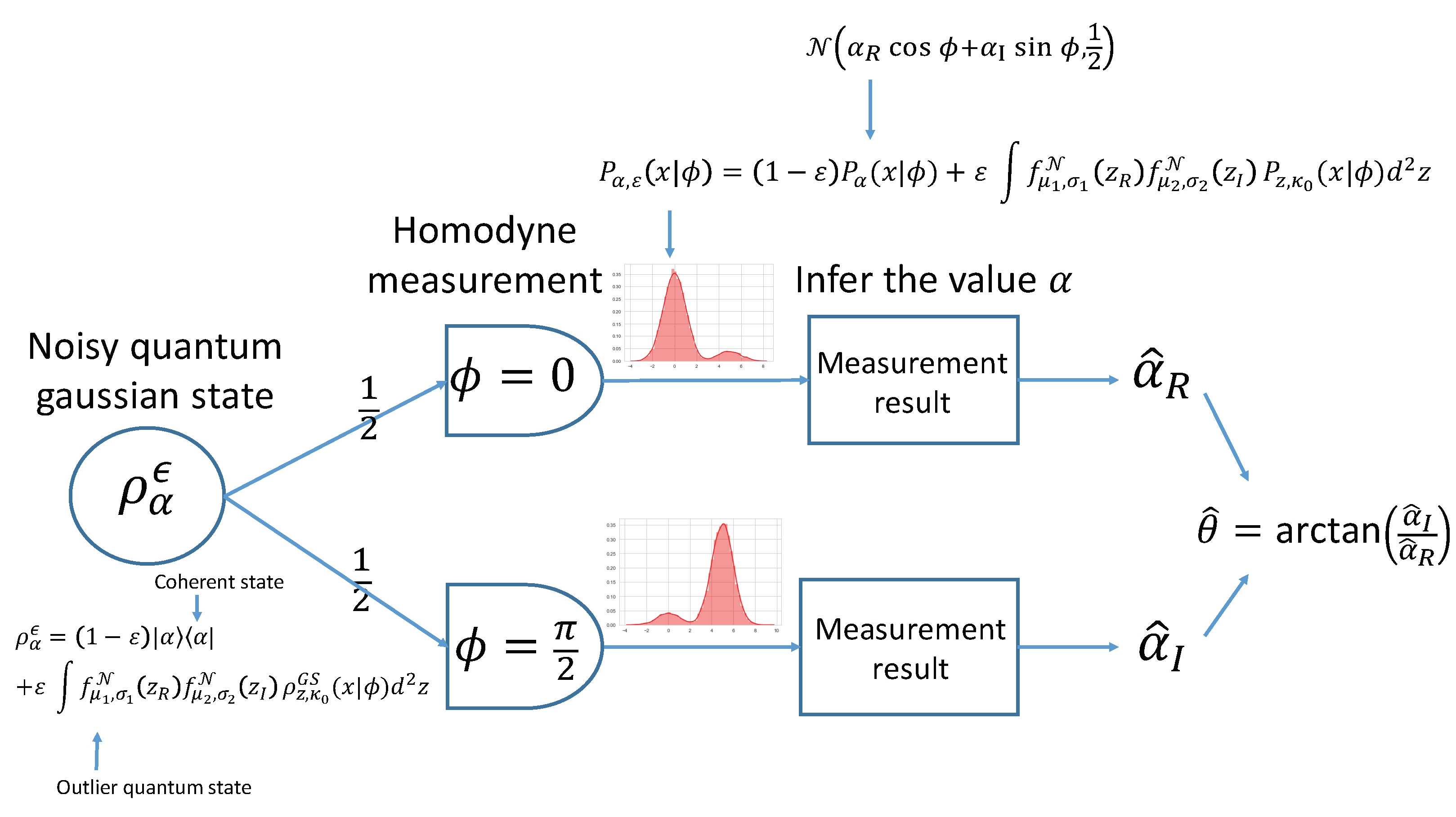
To illustrate advantages of the M-estimator in noisy quantum gaussian systems, we consider a phase estimation problem, which has many important applications for quantum information processing protocols [28,29,30,31,32,33,34,35]. Suppose an unknown coherent state is given. Importantly, the ideal state is parametrized by two real parameters ( and ). Our primary interest is to estimate the phase of an unknown coherent state . In our setting, the phase is the parameter of interest and the other parameter, the amplitude of the state, is the nuisance parameter of the model [26,27]. The optimal estimation strategy for this problem is known. However, this optimal measurement depends on the unknown phase and cannot be implemented. In the following, we consider a random mixture of two homodyne measurements at . As an estimator, we first apply M-estimators to infer the value . We then convert it to phase by:
A schematic diagram of our setting is given in Figure 1.
5.1. Numerical Simulation
We will now describe procedures of our numerical simulation. We set the true coherent state as . The true phase value is . We randomly generate n quantum gaussian states, which is a convex mixture of the ideal coherent state and outlier quantum states (either a single outlier quantum state case (29) or a distributed outlier quantum state case (30)). We perform a random homodyne measurements at with equal probability. From measurement outcomes at , we apply an M-estimator to estimate . The imaginary part will be estimated by homodyne measurement at . We repeat the iterative algorithm of Section 2.3 to obtain estimates. We stop iteration when the difference between two successive estimates is below a predetermined threshold value. We then apply the formula (37) to obtain an estimate . In our simulation, we change the sample size n for a given contamination parameter . We compare two types of M-estimators (bisquare and gamma) together with the sample mean and the median. (The sample mean for the ideal coherent state corresponds to the MLE in our setting).
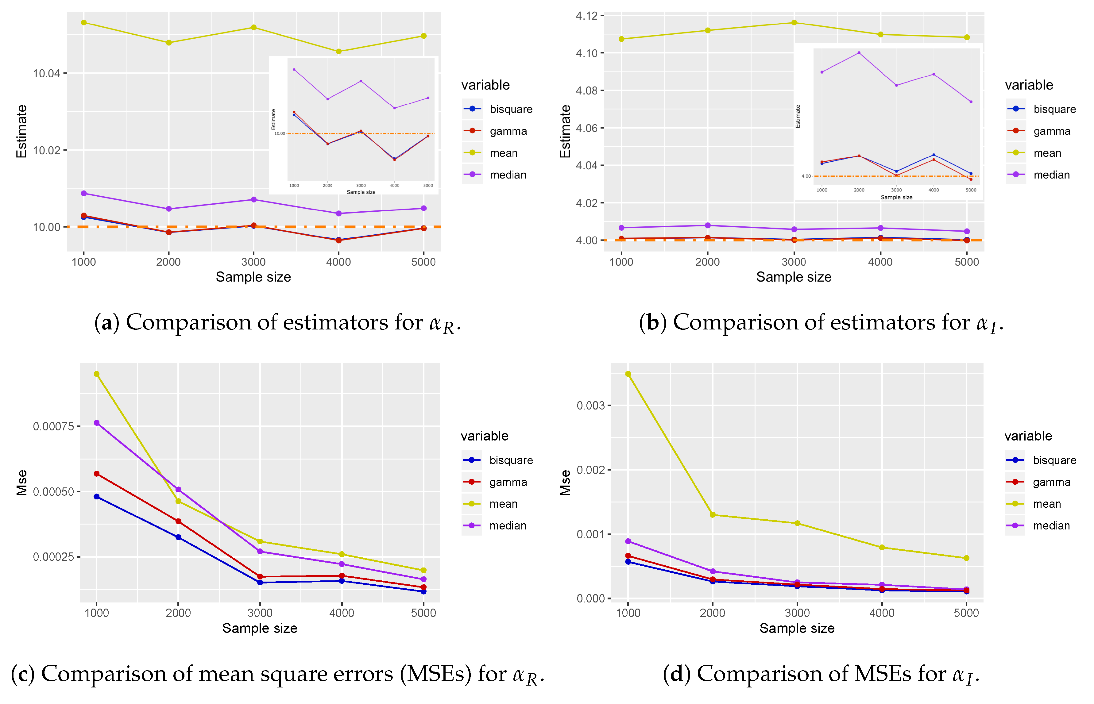
5.2. Single Outlier Quantum State
An outlier quantum state is set as in Equation (29). We first change the sample size to analyze performances of M-estimators for the contamination parameter . Comparisons of M-estimators and vs. the sample size n are plotted in Figure 2a,b, respectively. In Figure 2c,d, we plot the mean square errors (MSEs) of these estimators vs. the sample size n for the contamination parameter . In these figures, estimates from the sample mean (yellow-green), the median (purple), bisquare M-estimator (blue), and gamma M-estimator (red) are plotted, averaged over 500 runs of each setting. The true values are plotted by a dashed-dotted line (orange). From Figure 2a,b, we can see that the bisqure and gamma M-estimators both performed well when compared to the sample mean and the median. The observed differences between these two figures come from the fact that is harder to estimate than . This is because measurement outcomes at are more sensitive to outlier quantum states, as the two gaussian distributions are close to each other. Good performances in the MSEs were also observed for the bisqure and gamma M-estimators, as shown in Figure 2c,d. We should stress that the mean and the median are not consistent estimators for our setting.
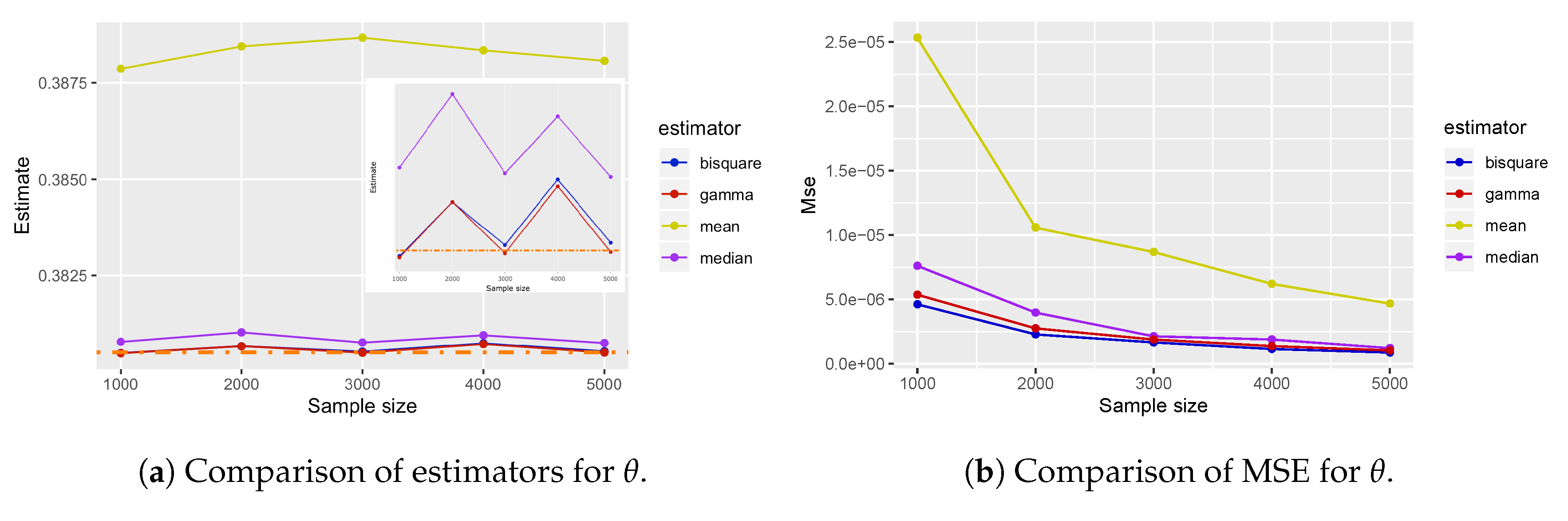
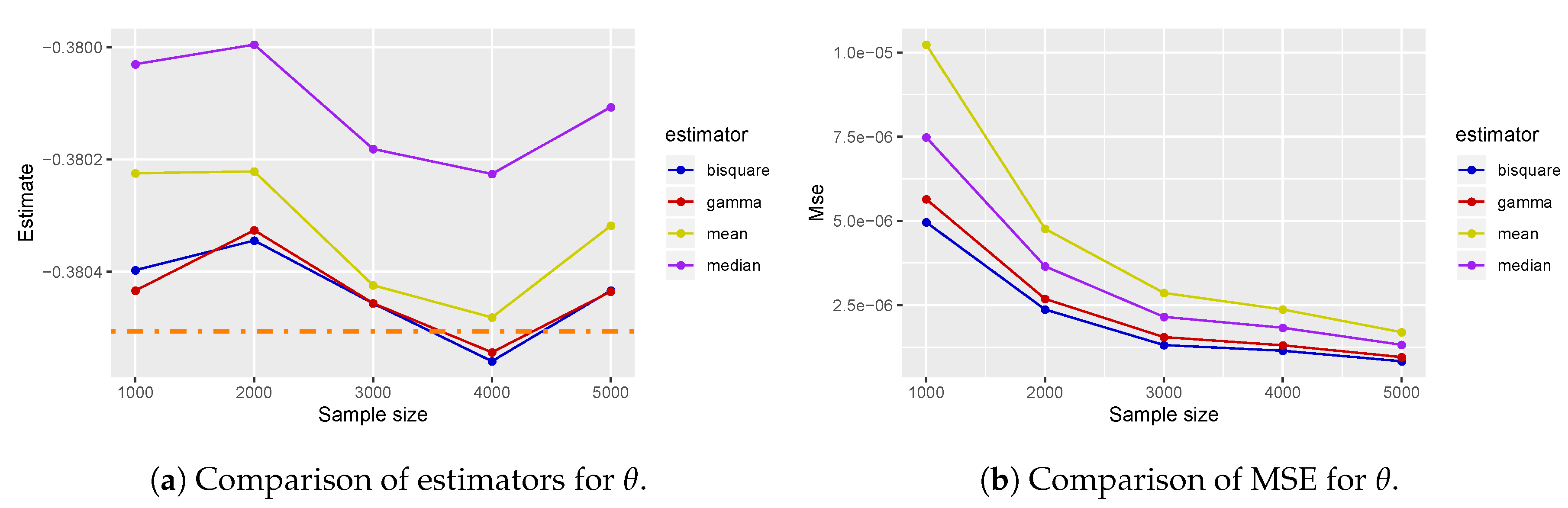
Next, we plot the result for phase estimation in Figure 3. The same convention as in Figure 2 is used. From Figure 3a,b, we draw the same conclusions for the bisqure and gamma M-estimators as in Figure 2. Namely, they are robust and consistent estimators. This is well understood from the fact that it is sufficient to have good estimators for and to estimate phase accurately.
5.3. Robustness of M-estimators
We will now analyze the robustness of the two M-estimators, the sample mean, and the median. First, we analyzed the FBP (14) for phase estimation, as shown in Figure 4. To produce this figure, we randomly replaced data with artificial data, which were generated by the normal distribution . The step size for increasing the number of replacing outliers (outlier counts) is 250 in Figure 4. In this setting, an estimator is regarded as being outside the parameter space when it returns the value . This corresponds to and being close to 1000.
Based on this figure, FBPs for four estimators were roughly estimated as follows: mean = 1500/5000 = 0.3, bisquare = 1750/5000 = 0.35, gamma and median = 2750/5000 = 0.55. From a first glance at this figure, we might conclude that the median and gamma M-estimators are robust estimators. However, we already know from Figure 3 that the median does not show consistency as an estimator. This discrepancy is easily resolved by realizing that the definition of the FBP is not related to the actual estimate at all. From this simple example, we conclude that the FBP should not be used as a measure of robustness a priori.
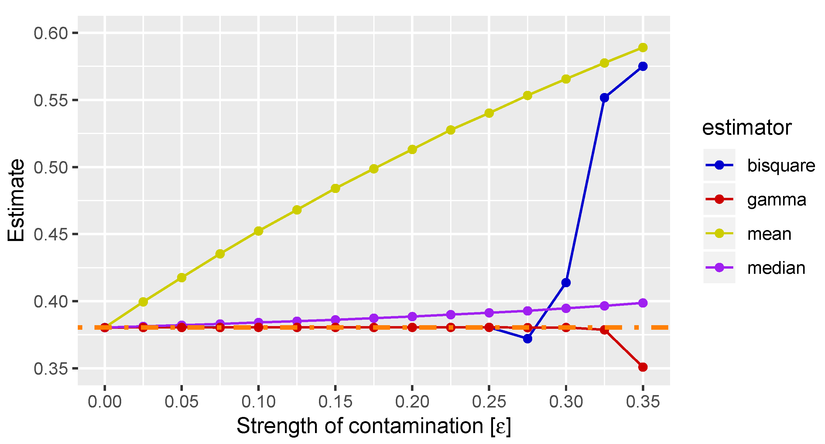
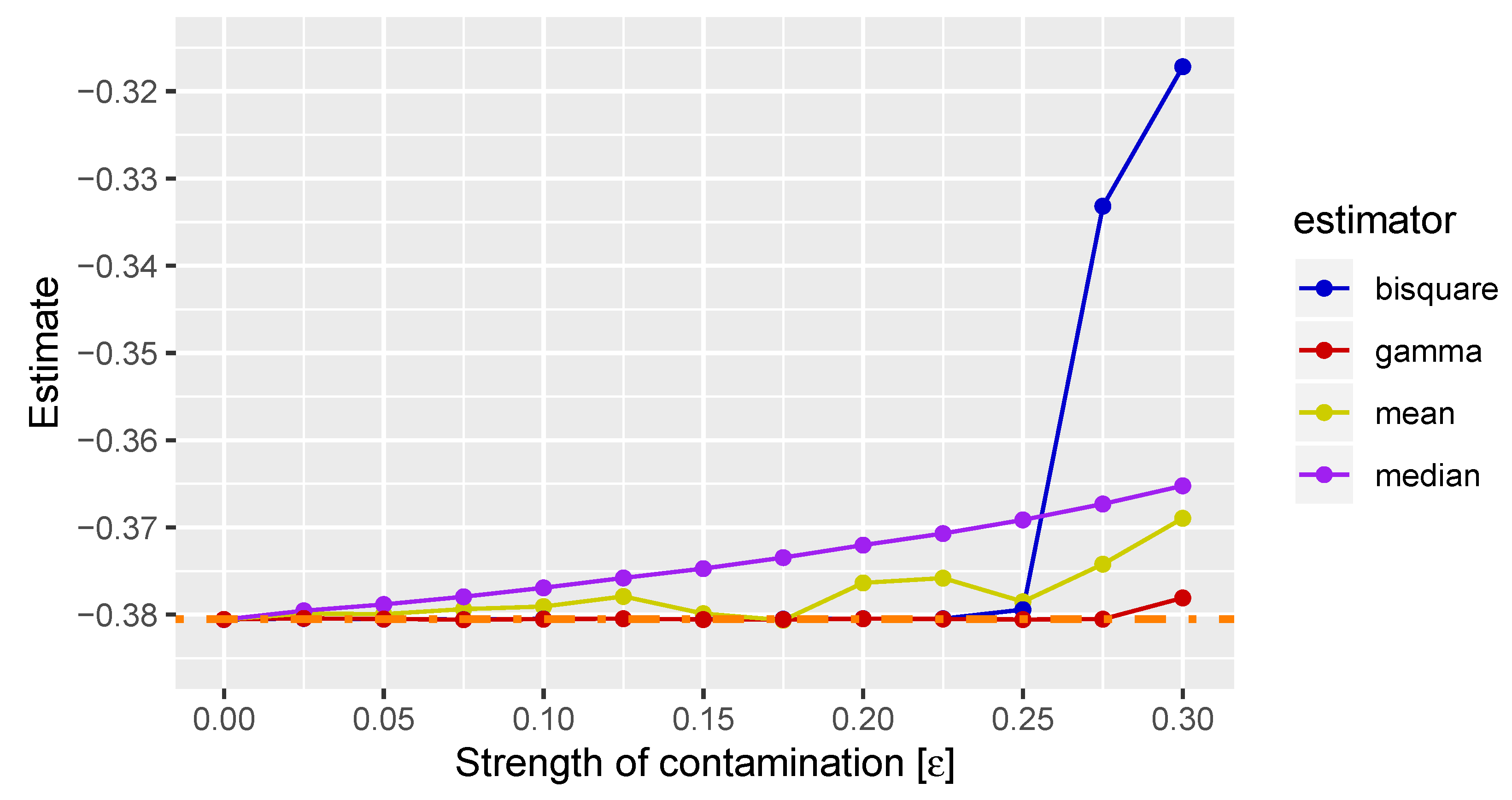
Next, we plotted the -curve proposed at the end of Section 3. This is to plot behaviors of an M-estimator as a function of the contamination parameter for a fixed sample size. In Figure 5, we show the -curve for phase estimation for the sample size . From this figure, we find that gamma M-estimators were the most robust estimators for small . By contrast, the sample mean and the median smoothly deviated from the true value. However, it is noted that the bisquare and gamma M-estimators behaved in uncontrollable manners after some threshold: for bisquare and for gamma.
Before we move to the next subsection, we report the average number of iterations of the M-estimator algorithm in Table 1 and Table 2. From the two tables, we see that the number of iterations needed to get a robust estimate was relatively small. This shows that the M-estimator can be implemented efficiently.
5.4. Distributed Outlier Quantum States
We will now consider a more general setting where outlier quantum states are distributed around the vacuum state of the form Equation (30). Outlier quantum states are generated according to the normal distribution as , with a fixed value of dispersion . We set the true coherent state as in this example. The true phase value is . In Figure 6, we show the performances of the M-estimators together with the sample mean and the median for the contamination parameter . The same convention as in Figure 2 is used. From Figure 6, we observe that the bisquare and gamma M-estimators performed well compared to other estimators. In this class of outlier quantum states, the median seems to be a bad choice to use. In fact, its performance was worse than that of the sample mean.
Finally, we analyzed the robustness of M-estimators by the -curve. In Figure 7, we plot the -curve for phase estimation of the sample size . From this result, we found that the gamma M-estimator was most robust and the bisquare M-estimator was second. The sample mean was also found to be relatively robust with small fluctuation. However, this behavior in fact depends on the nature of outlier quantum states as discussed in the next subsection. Lastly, the result of the median showed that it is not trustable for the distributed outlier quantum states of this kind.
5.5. Discussion
Following the two reasons described below, we conclude that the gamma M-estimator is the most robust estimator in comparison to the mean, median, and the well-known robust estimator bisquare, upon estimating the phase of the coherent state. First, from Figure 3a and Figure 6a, gamma was better than the other estimators in terms of accuracy in estimating the phase . Second, -curves (Figure 5 and Figure 7) suggest that the gamma M-estimator was the best in terms of robustness as well.
From the MSE plots (Figure 3b and Figure 6b), it was confirmed that the gamma estimator and the bisquare estimator had similar convergence speeds. Furthermore, from Table 1 and Table 2, it was found that the iteration of the robust estimation algorithm was suppressed to 10 or less for both gamma and bisquare before breakdown. In Figure 6a, relatively good accuracy of the mean estimation was observed. This is because of the effect of the nuisance parameter in our model. In fact, the sample means for and behaved very poorly with large biases. However, the errors of each estimation of and were canceled out. This then yielded an improvement in estimating the phase . We remark that this kind of an accidental improvement can only happen in a special case. When we do not have prior knowledge on possible outlier quantum states, M-estimators give more robust and reliable estimates.
6. Conclusions and Outlook
In this paper, we studied the problem of phase estimation for coherent states in the presence of unavoidable outlier quantum states. Measurement outcomes were then distributed according to a convex mixture of the ideal distribution and noisy distributions due to outliers. To overcome this problem, the methodology of M-estimators was introduced based on the well-established theory of robust statistics. Two specific M-estimators, bisquare and gamma, were studied to illustrate the advantage over conventional estimators. We found that the gamma M-estimator is most accurate as well as robust against the effect of outlier quantum states.
Before closing our paper, we would like to make a few remarks regarding future works. Our formalism applies to more general estimation settings with a quantum gaussian state, such as squeezed states and entangled states. This is done by replacing the ideal state, a coherent state, by other states of interest in Equation (28). More general quantum contaminated models can be treated without any modification. Preliminary studies showed that M-estimators work efficiently in this case as well. Our quantum statistical model in the presence of outlier quantum states can also be used to model imperfections in other elements of quantum information processing, such as gate operations and measurement processes. In this sense, the proposed method of M-estimators has wider applications to overcome certain types of SPAM errors in practice. Last, we mainly considered a quantum communication scenario in this paper. Utilization of robust statistics should be relevant to handle the problem of outlier quantum states when implementing other high precision measurement schemes based on quantum resources, such as quantum metrology, quantum imaging, and quantum sensing.
Author Contributions
Conceptualization, Y.M. and J.S.; software, Y.M.; formal analysis, Y.M. and J.S.; writing—original draft preparation, Y.M. and J.S.; writing—review and editing, Y.M. and J.S.; visualization, Y.M.; supervision, J.S.; funding acquisition, J.S. All authors have read and agreed to the published version of the manuscript.
Funding
The work is partly supported by JSPS KAKENHI grant number JP17K05571.
Conflicts of Interest
The authors declare no conflict of interest.
References
- Merkel, S.T.; Gambetta, J.M.; Smolin, J.A.; Poletto, S.; Córcoles, A.D.; Johnson, B.R.; Ryan, C.A.; Steffen, M. Self-consistent quantum process tomography. Phys. Rev. A 2013, 87, 062119. [Google Scholar] [CrossRef] [Green Version]
- Ferrie, C. Self-guided quantum tomography. Phys. Rev. Lett. 2014, 113, 190404. [Google Scholar] [CrossRef] [PubMed] [Green Version]
- Sugiyama, T.; Imori, S.; Tanaka, F. Reliable characterization of super-accurate quantum operations. arXiv 2018, arXiv:1806.02696. [Google Scholar]
- Huber, P.J. Robust Statistics; John Wiley & Sons: Hoboken, NJ, USA, 2004; Volume 523. [Google Scholar]
- Andrews, D.; Hampel, F. Robust Estimates of Location: Survey and Advances; Princeton University Press: Princeton, NJ, USA, 2015. [Google Scholar]
- Wilcox, R.R. Introduction to Robust Estimation and Hypothesis Testing; Academic Press: Cambridge, MA, USA, 2011. [Google Scholar]
- Hampel, F.R.; Ronchetti, E.M.; Rousseeuw, P.J.; Stahel, W.A. Robust Statistics: The Approach Based on Influence Functions; John Wiley & Sons: Hoboken, NJ, USA, 2011; Volume 196. [Google Scholar]
- Maronna, R.A.; Martin, R.D.; Yohai, V.J.; Salibián-Barrera, M. Robust Statistics: Theory and Methods (with R); John Wiley & Sons: Hoboken, NJ, USA, 2019. [Google Scholar]
- Wasserstein, R.L.; Lazar, N.A. The ASA Statement on p-Values: Context, Process, and Purpose. Am. Stat. 2016, 70, 129–133. [Google Scholar] [CrossRef] [Green Version]
- Camerer, C.F.; Dreber, A.; Holzmeister, F.; Ho, T.H.; Huber, J.; Johannesson, M.; Kirchler, M.; Nave, G.; Nosek, B.A.; Pfeiffer, T.; et al. Evaluating the replicability of social science experiments in Nature and Science between 2010 and 2015. Nat. Hum. Behav. 2018, 2, 637–644. [Google Scholar] [CrossRef] [Green Version]
- Wasserstein, R.L.; Schirm, A.L.; Lazar, N.A. Moving to a World Beyond “p < 0.05”. Am. Stat. 2019, 73, 1–19. [Google Scholar] [CrossRef] [Green Version]
- Braunstein, S.L.; Van Loock, P. Quantum information with continuous variables. Rev. Mod. Phys. 2005, 77, 513. [Google Scholar] [CrossRef] [Green Version]
- Wang, X.B.; Hiroshima, T.; Tomita, A.; Hayashi, M. Quantum information with Gaussian states. Phys. Rep. 2007, 448, 1–111. [Google Scholar] [CrossRef] [Green Version]
- Serafini, A. Quantum Continuous Variables: A Primer of Theoretical Methods; CRC Press: Boca Raton, FL, USA, 2017. [Google Scholar]
- Fujisawa, H.; Eguchi, S. Robust parameter estimation with a small bias against heavy contamination. J. Multivar. Anal. 2008, 99, 2053–2081. [Google Scholar] [CrossRef] [Green Version]
- Helstrom, C.W. The minimum variance of estimates in quantum signal detection. IEEE Trans. Inf. Theory 1968, 14, 234–242. [Google Scholar] [CrossRef]
- Helstrom, C.W. Quantum detection and estimation theory. J. Stat. Phys. 1969, 1, 231–252. [Google Scholar] [CrossRef] [Green Version]
- Helstrom, C.W.; Kennedy, R. Noncommuting observables in quantum detection and estimation theory. IEEE Trans. Inf. Theory 1974, 20, 16–24. [Google Scholar] [CrossRef] [Green Version]
- Yuen, H.; Lax, M. Multiple-parameter quantum estimation and measurement of nonselfadjoint observables. IEEE Trans. Inf. Theory 1973, 19, 740–750. [Google Scholar] [CrossRef]
- Helstrom, C.W. Quantum Detection and Estimation Theory; Academic Press: Cambridge, MA, USA, 1976. [Google Scholar]
- Holevo, A.S. Probabilistic and Statistical Aspects of Quantum Theory; Edizioni della Normale: Pisa, Italy, 2011. [Google Scholar]
- Fujiwara, A.; Nagaoka, H. An estimation theoretical characterization of coherent states. J. Math. Phys. 1999, 40, 4227–4239. [Google Scholar] [CrossRef]
- D’ariano, G.M.; Paris, M.G.; Sacchi, M.F. Parameter estimation in quantum optics. Phys. Rev. A 2000, 62, 023815. [Google Scholar] [CrossRef] [Green Version]
- Paris, M.G.A.; Řeháček, J.E. Quantum State Estimation; Springer: Berlin, Germany, 2004. [Google Scholar]
- Hayashi, M. Quantum Information Theory. In Graduate Texts in Physics; Springer: Berlin, Germany, 2017. [Google Scholar]
- Suzuki, J. Nuisance parameter problem in quantum estimation theory: Tradeoff relation and qubit examples. J. Phys. A: Math. Theor. 2020, 53, 264001. [Google Scholar] [CrossRef]
- Suzuki, J.; Yang, Y.; Hayashi, M. Quantum state estimation with nuisance parameters. J. Phys. A Math. Theor. 2020. [Google Scholar] [CrossRef]
- Aspachs, M.; Calsamiglia, J.; Muñoz-Tapia, R.; Bagan, E. Phase estimation for thermal Gaussian states. Phys. Rev. A 2009, 79, 033834. [Google Scholar] [CrossRef] [Green Version]
- Pinel, O.; Jian, P.; Treps, N.; Fabre, C.; Braun, D. Quantum parameter estimation using general single-mode Gaussian states. Phys. Rev. A 2013, 88, 040102. [Google Scholar] [CrossRef] [Green Version]
- Bradshaw, M.; Lam, P.K.; Assad, S.M. Ultimate precision of joint quadrature parameter estimation with a Gaussian probe. Phys. Rev. A 2018, 97, 012106. [Google Scholar] [CrossRef] [Green Version]
- Oh, C.; Lee, C.; Rockstuhl, C.; Jeong, H.; Kim, J.; Nha, H.; Lee, S.Y. Optimal Gaussian measurements for phase estimation in single-mode Gaussian metrology. Npj Quantum Inf. 2019, 5, 1–9. [Google Scholar] [CrossRef]
- Lee, C.; Oh, C.; Jeong, H.; Rockstuhl, C.; Lee, S.Y. Using states with a large photon number variance to increase quantum Fisher information in single-mode phase estimation. J. Phys. Commun. 2019, 3, 115008. [Google Scholar] [CrossRef]
- Arnhem, M.; Karpov, E.; Cerf, N.J. Optimal Estimation of Parameters Encoded in Quantum Coherent State Quadratures. Appl. Sci. 2019, 9, 4264. [Google Scholar] [CrossRef] [Green Version]
- Oh, C.; Lee, C.; Lie, S.H.; Jeong, H. Optimal distributed quantum sensing using Gaussian states. Phys. Rev. Res. 2020, 2, 023030. [Google Scholar] [CrossRef] [Green Version]
- Assad, S.M.; Li, J.; Liu, Y.; Zhao, N.; Zhao, W.; Lam, P.K.; Ou, Z.; Li, X. Accessible precisions for estimating two conjugate parameters using Gaussian probes. Phys. Rev. Res. 2020, 2, 023182. [Google Scholar] [CrossRef]
- Donoho, D.L.; Huber, P.J. The notion of breakdown point. In A Festschrift for Erich L. Lehmann; CRC Press: Boca Raton, FL, USA, 1983; pp. 157–184. [Google Scholar]
- Huber, P.J. Finite sample breakdown of M-and P-estimators. Ann. Stat. 1984, 12, 119–126. [Google Scholar] [CrossRef]
Figure 1.
A schematic diagram of our model and estimation procedure.

Figure 2.
Performances of M-estimators (bisquare and gamma) and the standard estimators (mean and median) as functions of the sample size.
Figure 2.
Performances of M-estimators (bisquare and gamma) and the standard estimators (mean and median) as functions of the sample size.

Figure 3.
Performances of M-estimators for phase estimation of a coherent state in the presence of a single outlier quantum state.
Figure 3.
Performances of M-estimators for phase estimation of a coherent state in the presence of a single outlier quantum state.

Figure 4.
The finite breakdown point (FBP) for estimating phase of a coherent state.

Figure 5.
-curve for phase estimation for the sample size .

Figure 6.
Comparison of estimators for .

Figure 7.
-curve for phase estimation for the sample size .


Table 1.
The average number of iterations of robust estimator algorithm for .
| 0 | 0.025 | 0.05 | 0.075 | 0.1 | 0.125 | 0.15 | 0.175 | 0.2 | 0.225 | 0.25 | 0.275 | 0.3 | 0.325 | 0.35 | |
| bisquare | 3.21 | 5.00 | 5.01 | 5.00 | 5.00 | 5.11 | 5.99 | 6.00 | 6.08 | 7.11 | 9.07 | 20.02 | 11.00 | 6.67 | 5.29 |
| gamma | 7.97 | 7.99 | 7.99 | 8.00 | 8.02 | 8.04 | 8.12 | 8.28 | 8.57 | 8.85 | 9.00 | 9.20 | 9.89 | 11.60 | 17.77 |
Table 2.
The average number of iterations of robust estimator algorithm for .
| 0 | 0.025 | 0.05 | 0.075 | 0.1 | 0.125 | 0.15 | 0.175 | 0.2 | 0.225 | 0.25 | 0.275 | 0.3 | 0.325 | 0.35 | |
| bisquare | 3.19 | 5.00 | 5.00 | 4.96 | 4.05 | 4.67 | 5.00 | 5.00 | 5.41 | 6.06 | 7.07 | 9.64 | 20.06 | 9.99 | 6.50 |
| gamma | 7.97 | 7.99 | 8.01 | 8.01 | 8.02 | 8.02 | 8.05 | 8.09 | 8.09 | 8.12 | 8.18 | 8.20 | 8.21 | 8.23 | 8.38 |
© 2020 by the authors. Licensee MDPI, Basel, Switzerland. This article is an open access article distributed under the terms and conditions of the Creative Commons Attribution (CC BY) license (http://creativecommons.org/licenses/by/4.0/).
Share and Cite
MDPI and ACS Style
Mototake, Y.; Suzuki, J. Robust Phase Estimation of Gaussian States in the Presence of Outlier Quantum States. Appl. Sci. 2020, 10, 5475. https://doi.org/10.3390/app10165475
AMA Style
Mototake Y, Suzuki J. Robust Phase Estimation of Gaussian States in the Presence of Outlier Quantum States. Applied Sciences. 2020; 10(16):5475. https://doi.org/10.3390/app10165475
Chicago/Turabian StyleMototake, Yukito, and Jun Suzuki. 2020. "Robust Phase Estimation of Gaussian States in the Presence of Outlier Quantum States" Applied Sciences 10, no. 16: 5475. https://doi.org/10.3390/app10165475
Note that from the first issue of 2016, this journal uses article numbers instead of page numbers. See further details here.