A Novel Adaptive Mode Decomposition Method Based on Reassignment Vector and Its Application to Fault Diagnosis of Rolling Bearing

1
Key Laboratory of Metallurgical Equipment and Control Technology, Ministry of Education, Wuhan University of Science and Technology, Wuhan 430081, China
2
Hubei Key Laboratory of Mechanical Transmission and Manufacturing Engineering, Wuhan University of Science and Technology, Wuhan 430081, China
3
Lishui Special Equipment Testing Institute, Lishui 323000, China
4
Taizhou Special Equipment Inspection and Testing Institute, Taizhou 318000, China
*
Author to whom correspondence should be addressed.
Appl. Sci. 2020, 10(16), 5479; https://doi.org/10.3390/app10165479
Submission received: 21 June 2020
/
Revised: 3 August 2020
/
Accepted: 5 August 2020
/
Published: 7 August 2020
(This article belongs to the Special Issue Bearing Fault Detection and Diagnosis)
Abstract
:To solve the problem that the random distribution of noise in the time-frequency (TF) plane largely affects the readability of TF representations, a novel signal adaptive decomposition algorithm processed in TF domain, which provides adequate information about the time-varying instantaneous frequency, is presented in this paper. The theoretical basis of this algorithm is short-time Fourier transform (STFT). The research into the algorithm comprises two steps: the TF plane denoising takes sparse low-rank matrix estimation as a priority and then achieves signal decomposition based on reassignment vector (RV). A low-rank matrix approximation scheme, which exploits the sparse properties of the TF transformation coefficient and uses non-convex penalty, is put forward to obtain clean STFT. Then, a new approach called RV, which is different from the traditional mode decomposition methods such as Empirical Mode Decomposition (EMD), is used to estimate the characteristic curve corresponding to the TF ridges of the interested modes. Based on the classical reassignment method, RV has a solid theory foundation. Moreover, it can identify different signal components such as stationary signal, modulating signal and impulse characteristic. Combining the advantages of low-rank matrix approximation approach and those of RV defined in TF plane, a novel signal adaptive decomposition method is proposed in this paper to identify fault characteristics. To illustrate the effectiveness of the method, fault signals of rolling bearing under stationary condition and time-varying speed are respectively analyzed.
1. Introduction
The dynamic response of the transmission component under time-varying conditions, which are recognized as the working environment for most mechanical equipment in the engineering field, will show strong non-stationarity [1,2,3]. Even in healthy conditions, the characteristic frequency and amplitude of vibration signals will vary with the operating conditions. If the transmission component fails, it will be impossible to determine whether the change of its dynamic response characteristics is caused by the failure or the varying working conditions. Therefore, one key constituent is to realize fault feature extraction and state identification under time-varying conditions [4,5].
Recently, some researchers have put forward a machine learning and statistical framework to solve the similar problem described in this paper. However, these methods are limited to practical application because mechanical failure is typically a small sample situation [6,7,8]. As a very powerful signal processing method, time-frequency (TF) analysis has drawn much attention among researchers in structural health monitoring, biomedicine and other fields [9,10]. The main reason for this is its simultaneous examination for the complicated signals on two scales of time and frequency. Built on the inner product operation between the analytical signal and basis function [11,12,13], traditional TF analysis methods, such as Fast Fourier transform (FFT) and Wavelet Transform (WT), can neither match the time-varying signals well, nor effectively process the non-stationary signals. Moreover, the multi-component signals always contain heavy background noise. Therefore, the characteristic components are easily masked by irrelevant signals, and thus Short-time Fourier transform (STFT) and Wigner distribution (WD) have been proposed [14,15]. Despite an improved version of FFT, STFT remains within the limits of implementing adaptive selection of window function [16] and, inevitably, cross interference feature of WD inevitably exists, which directly leads to poor readability of the TF plane.
Recently, Synchrosqueezing Transform (SST) and Linear Chirp Transform (LCT) have become research hotspots [17,18]. As a post-processing method, SST has made it possible to synchrosqueeze and rearrange the TF coefficients along the frequency axis, which aimed to realize the concentration of TF energy [19]. Subsequently, several interesting methods have been presented, such as Synchroextracting Transform (SET) and Second order Synchrosqueezing Transform [20,21]. These methods, however, fail to analyze the strong modulated signal with heavy noise. Since the TF coefficient rearrangement is executed from the frequency direction, it has poor processing ability for the common impulse signal of mechanical equipment. Different from SST, LCT generates a rotation angle through a fixed rotation operator for the horizontal window in STFT. When the angle between the rotated window function and the frequency modulated signal is zero, the best energy concentration is reached [22]. However, when the signal is nonlinear, the frequency modulation of the signal is time-varying. As a result, only one rotation operator cannot fully meet the requirements of energy concentration at all times. In general, when dealing with nonlinear and non-stationary signals, the energy divergence problem is unavoidable in the above methods.
Reassignment method (RM) realizes the reallocation of TF transformation coefficients in two directions of time and frequency [23]. Compared with previous methods, RM not only has a higher TF resolution but it also reaches the ideal TF representations more easily. However, RM does not support signal reconstruction [24]. Moreover, the information extracted from the distribution parameters of the ridges, which are utilized for decomposing signal and reconstructing useful one, is closely related to the instantaneous frequency variation of the signal. Inspired by these views, this paper studies a signal adaptive decomposition algorithm on the basis of the theoretical framework of RM. By the theoretical calculation from RM, Reassignment Vector (RV) can identify the main TF ridges, representing the different mode components of the composed signal [25,26]. Different from the adaptive decomposition algorithm of one-dimensional signal such as Empirical Mode Decomposition (EMD) and Variational Mode Decomposition (VMD) [27,28], RV is proposed from two-dimensional TF presentations and behaves better in extracting the strong time-varying amplitude modulation and frequency modulation (AM/FM) modes. More importantly, compared with the above-mentioned methods, it has greater decomposition ability for impulse signal, which is of outstanding significance for structural health monitoring. For the further improvement of the decomposition performance of multi-component vibration signal, this paper also presents a TF plane denoising method, which is based on the existence in the form of matrix and an obvious sparsity of the TF transformation coefficient. Through the non-convex penalty function and convex optimization framework, the desired coefficient matrix, or clean TF plane, can be obtained by sparse low-rank matrix estimation [29,30]. Afterwards, RV is employed to identify different modes from the denoised TF representations. Combining the superiority of low-rank matrix approximation and RV, a novel signal adaptive decomposition algorithm is proposed to extract different fault mode components under diverse working conditions.
The rest of this paper contains four parts. Section 2 elaborates on the proposed method, especially TF plane denoising using sparse low-rank matrix estimation and adaptive signal decomposition based on reassignment vector. In the following section, simulation analysis with multi-components will be used for verifying the effectiveness of the raised method in signal adaptive decomposition. In Section 4, the vibration signal of rolling bearing with inner ring fault under constant condition and time-varying speed were used for experimental verification. Finally, Section 5 contains the conclusion.
2. Theory Description
2.1. TF Plane Denoising Using Sparse Low-rank Matrix Estimation
Commonly, multicomponent signal is defined as a superimposition of AM-FM components. The raw TF plane can be obtained by classical STFT and the TF transformation coefficient is expressed as a matrix. In this paper, the problem of estimating a sparse low-rank matrix from a noisy TF transformation coefficient of STFT is firstly addressed. The mathematical model of low-rank matrix approximation can be illustrated as follows:
where is the noise observation matrix computed by STFT, represents additive white Gaussian noise (AWGN) matrix and is corresponding to sparse low-rank matrix estimation of raw STFT. In order to estimate the sparse low-rank matrix , the model has been transformed into a typical mathematical optimization problem, which is composed of a data-fidelity term and two parameterized non-convex penalty functions [31]. The specific formula is expressed as follows:
where , is the non-convex penalty function, represents the singular values of the matrix , regularization parameters and are used to adjust weights between data-fidelity term and constraint term. The most commonly used penalty functions can be defined as:
The proximity operator of penalty function is defined as follows:
To ensure that the target function is strictly convex, the selected parameters need to satisfy the following conditions:
The objective function in formula (2) can be solved by alternating direction method of multipliers (ADMM) to achieve the separation of variables [32]. Then, the sparse low-rank matrix estimation of STTF transformation coefficient can be obtained for the following TF signature identification and signal adaptive decomposition.
2.2. Adaptive Signal Decomposition Based on Reassignment Vector
Reassignment method (RM) realizes the TF representation of multicomponent signals in two directions of time and frequency scale. In other words, RM can accurately position the TF signature of the interested modes. Based on the denoising operation in STFT domain defined in Section 2.1, the group delay estimation and instantaneous frequency estimation can be calculated as:
where and are corresponding to the denoised STFT operation using sparse low-rank matrix approximation of multicomponent signal calculated by the window function and . and is illustrated as the real and imaginary part of the complex number. Therefore, RM algorithm can be described as:
From the formula (9), we find that the RV is also considered in terms of time and frequency. If is satisfied, , which indicates that the component is existing along the time axis. Similarly, if f is a pure harmonic signal such as , , which demonstrates a component only along the frequency directions. More generally, a linear chirp signal is described with phase function and window function , thus we can obtain the RV as follows:
Generally speaking, RV points to that characteristic curve in the TF plane following the direction . Theoretically, on the basis of the projection of RV in a specific direction, contour points (CPs) representing the TF curve or intrinsic component can be obtained for the subsequent mode function extraction. Obviously, RV will exhibit a strong variation along the orientation by crossing the ridge curve. To determine the projection of RV in a specific direction, the key step is to get the angle . For the convenience of discretization and computation, RV can be regarded as a displacement on a grid. Then, the STFT is computed at frequencies , where and is the number of frequency bins. By the way above, the grid is indexed by and is corresponding to the time instant. Through the above theoretical definition, the CPs can be computed by projecting this vector following the inner product operation:
where is denoted as the vector along the direction . Based on it, a local projection angles (LPAs) algorithm published in [25] is used to achieve a robust estimation of TF signatures for a wide class of multicomponent signal. Using the just estimated CPs, each corresponding mode can be reconstructed through:
where is the basin of interested components corresponding to the mode i.
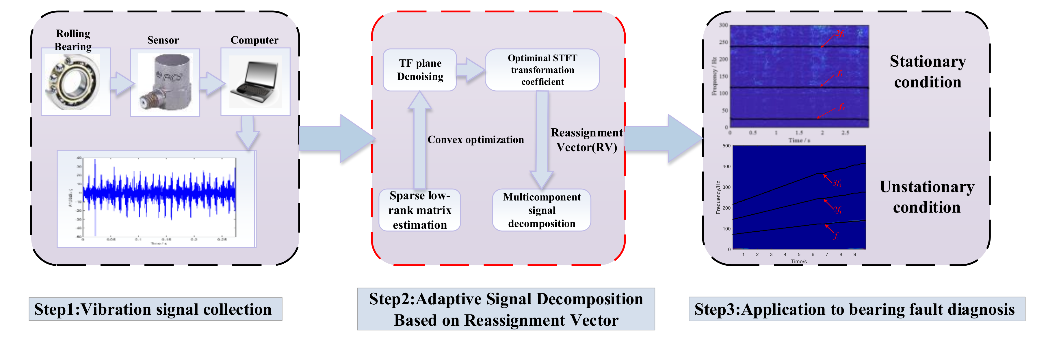
Taking advantage of sparse low-rank matrix estimation about transforming coefficient and reassignment vector pointing to ridge curve, a novel adaptive signal decomposition method is proposed in this paper. The specific process of the approach presented in this paper is shown in Figure 1.
3. Numerical Simulation Signal Analysis
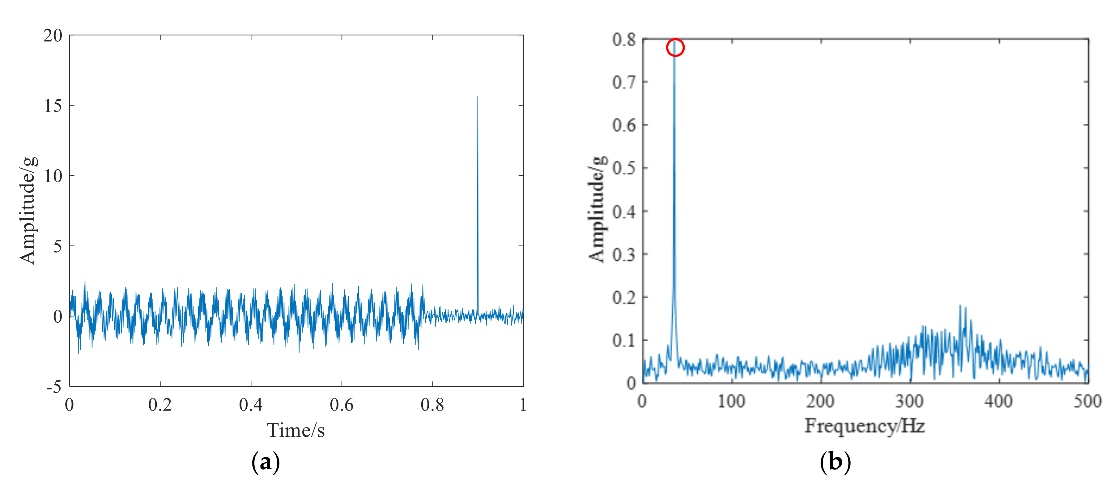
To prove that the raised method is effective, the numerical analysis performing is the priority. The simulated signal is composed by four parts including sinusoidal signal , modulated signal , impulse signal and noisy signal . It is designed to test its ability to process different types of signals.
where is the researched multi-component signal, the sampling number is 1024 and the sampling frequency is 1024 Hz. The characteristic frequency is set as and respectively. is the additive Gaussian noise components with dB. In terms of TF characteristics, has a constant frequency and has a strong time-varying frequency. The time-domain and frequency-domain waveform is shown in Figure 2. From the Figure 2a, we can clearly inspect the impulse characteristics in the time-domain. The frequency spectrum analysis result is plotted in Figure 2b, only the constant frequency has been identified with red circle, while the time-varying frequency feature and impulse feature remain undiscovered. It is demonstrated that the conventional analytical methods are not suitable for processing non-stationary signals.
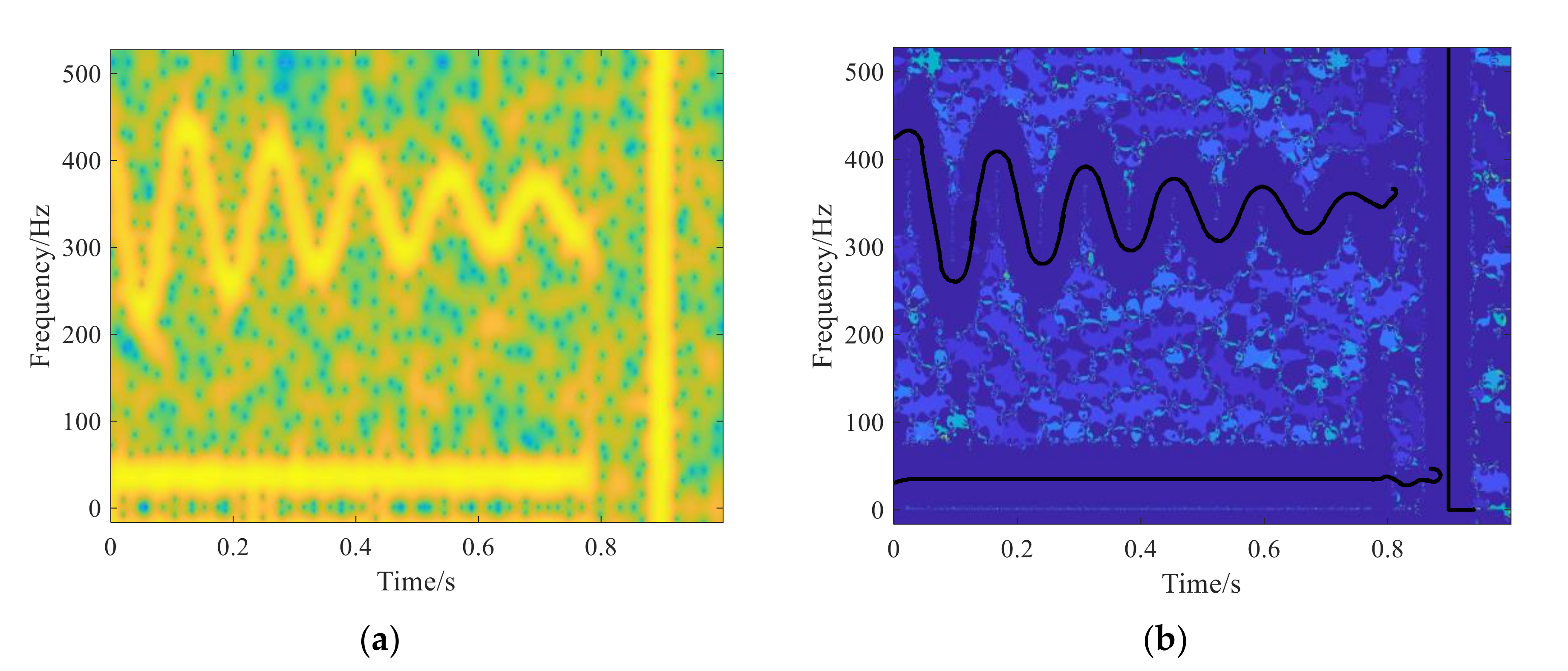
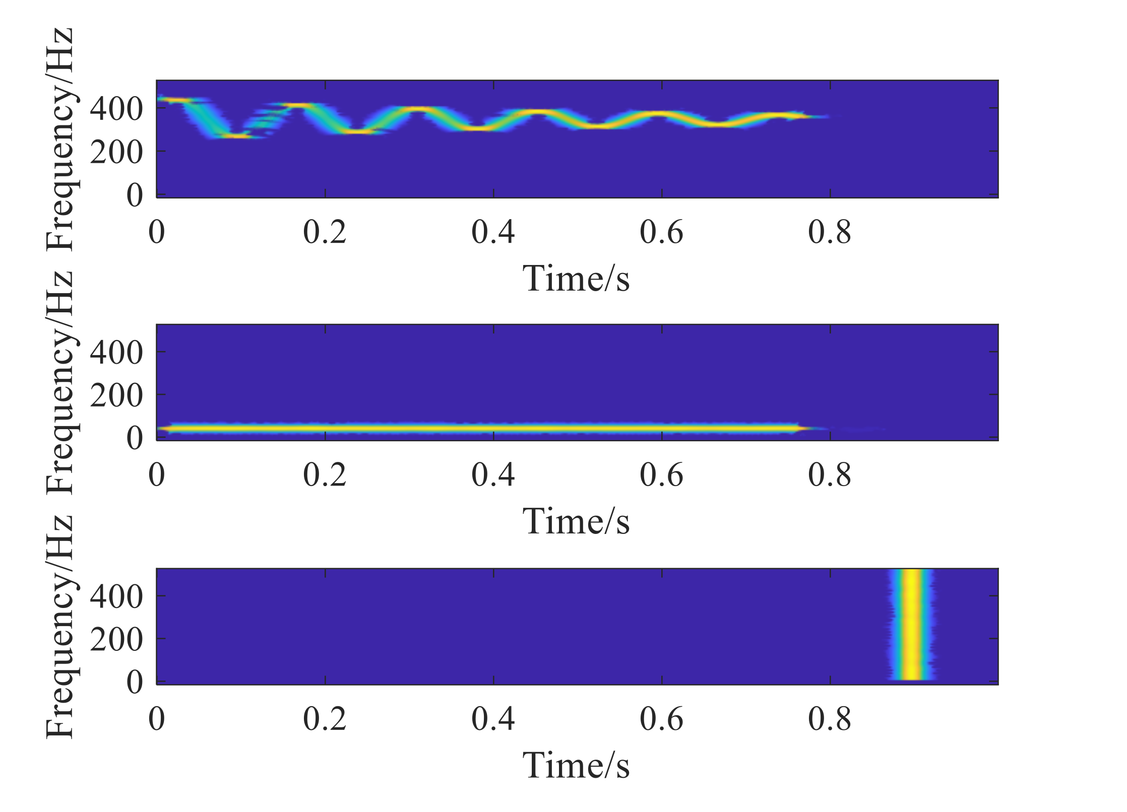
Then, the TF analysis methods, such as STFT and the proposed method using RV, are conducted to analysis multi-component simulated signal. The result is drawn in Figure 3. Due to the existence of noise components in the TF plane along the time and frequency direction as well as the theoretical defect, the time-frequency representations (TFR) generated by STFT is blurry, which is shown in Figure 3a. Essentially, the proposed method is based on time-frequency denoising scheme and rearrangement algorithm. Thus, it has better TF plane readability in the TF representations. Comparing Figure 3a with Figure 3b, it is obvious that the presented method can accurately extract the different signal characteristics. According to the identified TF feature of simulated signal, the adaptive signal mode decomposition from TF plane is plotted in Figure 4. Fortunately, different TF characteristics, including strong modulated and impulse, have been perfectly decomposed.
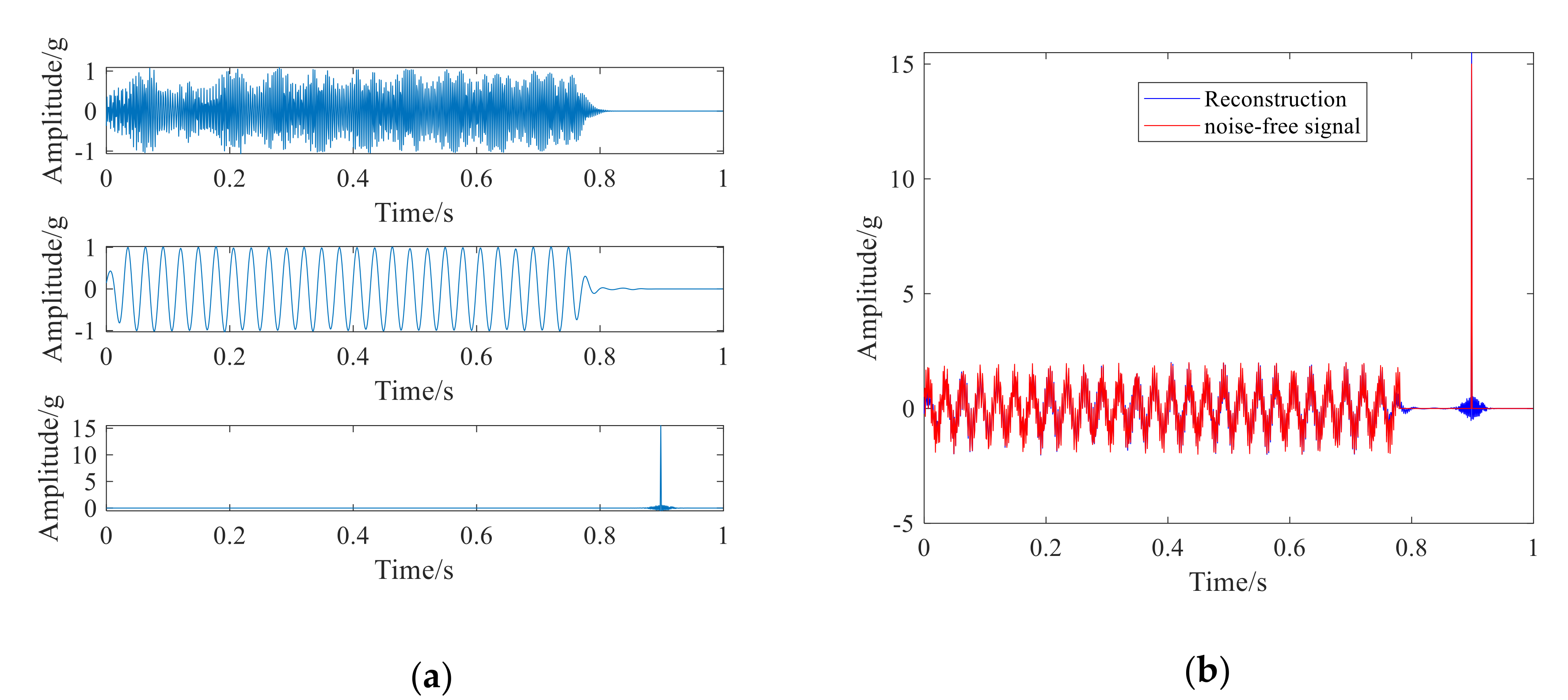
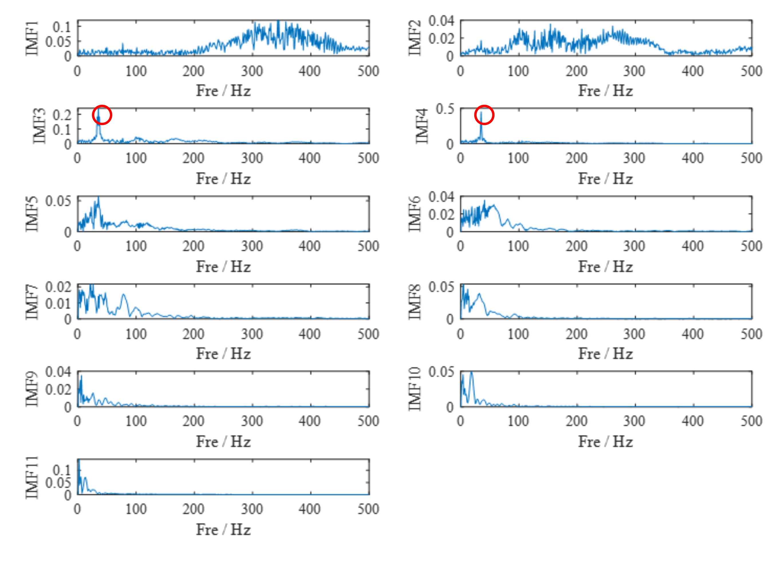
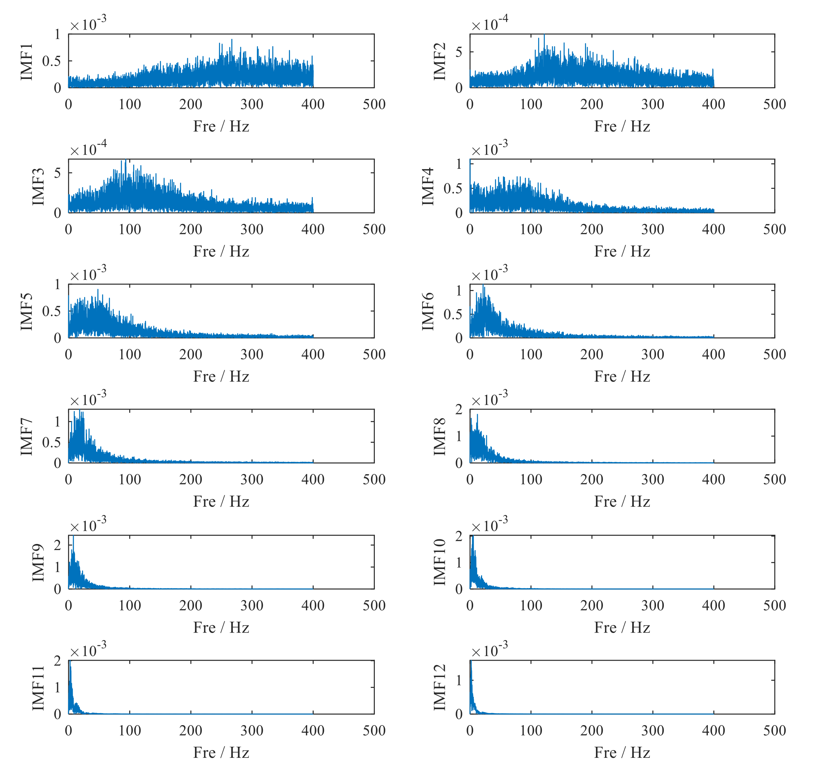
Subsequently, the multi-component signal decomposition and reconstruction operation on the basis of TF characteristics is performed. The computation result is shown in Figure 5 and we can draw a conclusion that the performance of the raised method has obvious superiority in signal decomposition. To compare performance of signal decomposition, the commonly used method of EMD is employed to decompose the simulated signal and the corresponding frequency spectrum analysis result is drawn in Figure 6. Only the constant frequency , which has been marked by a red circle, can be found in IMF3 and IMF4. The other signal components such as modulated signal and impulse signal still remain unidentified. Numerical simulation results show that the presented method is more suitable for the mode decomposition of different non-stationary components. It should be noted that the signal components must meet strict separation conditions in the TF domain described in [19], and thus the proposed method cannot fully separate close and overlapped signal components.
4. Experimental Data Analysis
4.1. Case.1 Application to Stationary Feature Extraction of Bearing
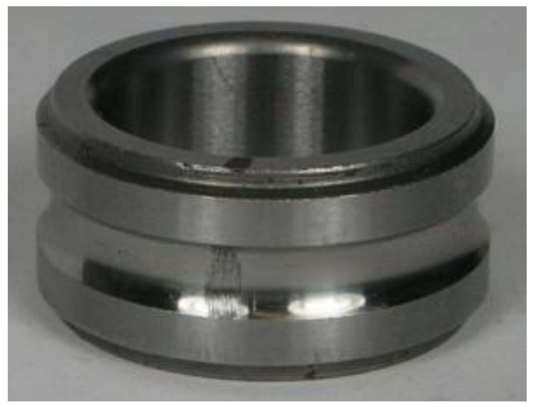
In the section of experimental data analysis, a public bearing fault dataset from Society for Machinery Failure Prevention Technology (MFPT) has been employed to verify the effectiveness of the proposed method [33]. The dataset is collected from a rolling bearing test rig with outer race fault and inner race fault at various loads. The inner race fault is selected as the research object in this paper as shown in Figure 7, and the detailed structure parameter of rolling bearing is listed in Table 1.
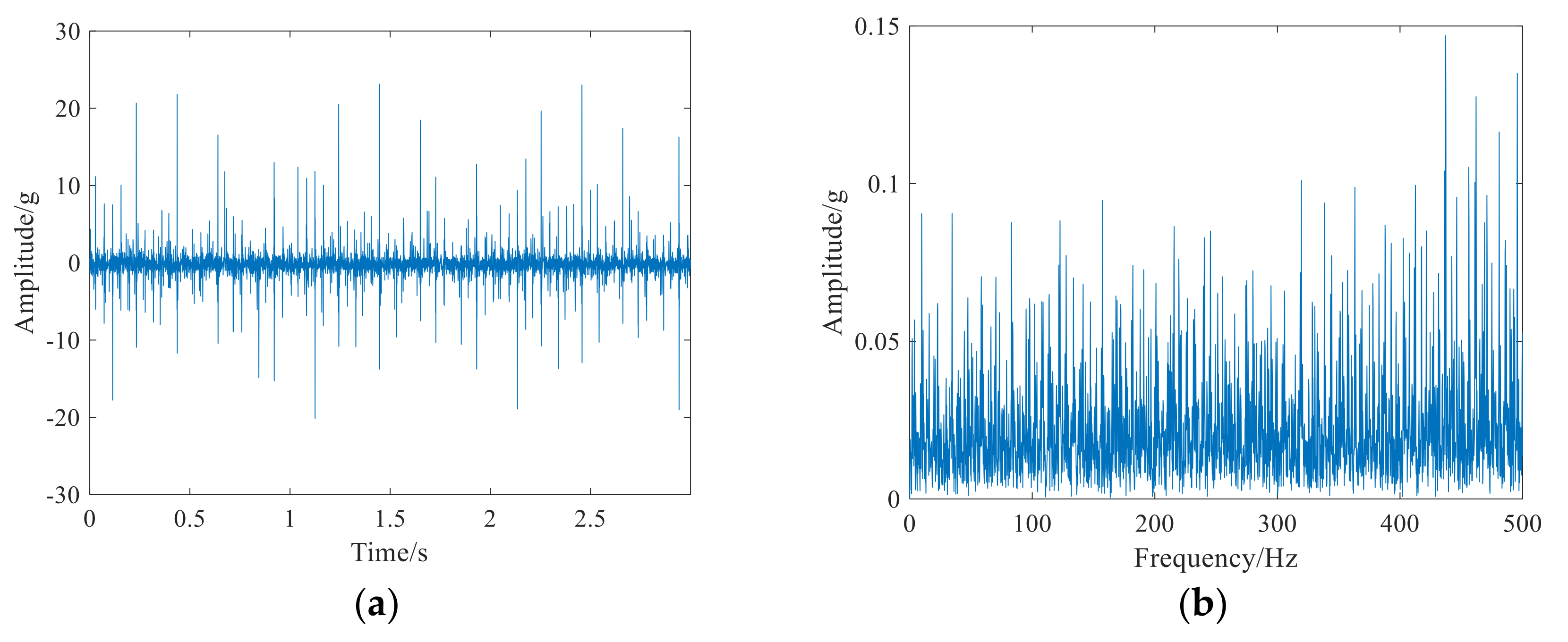
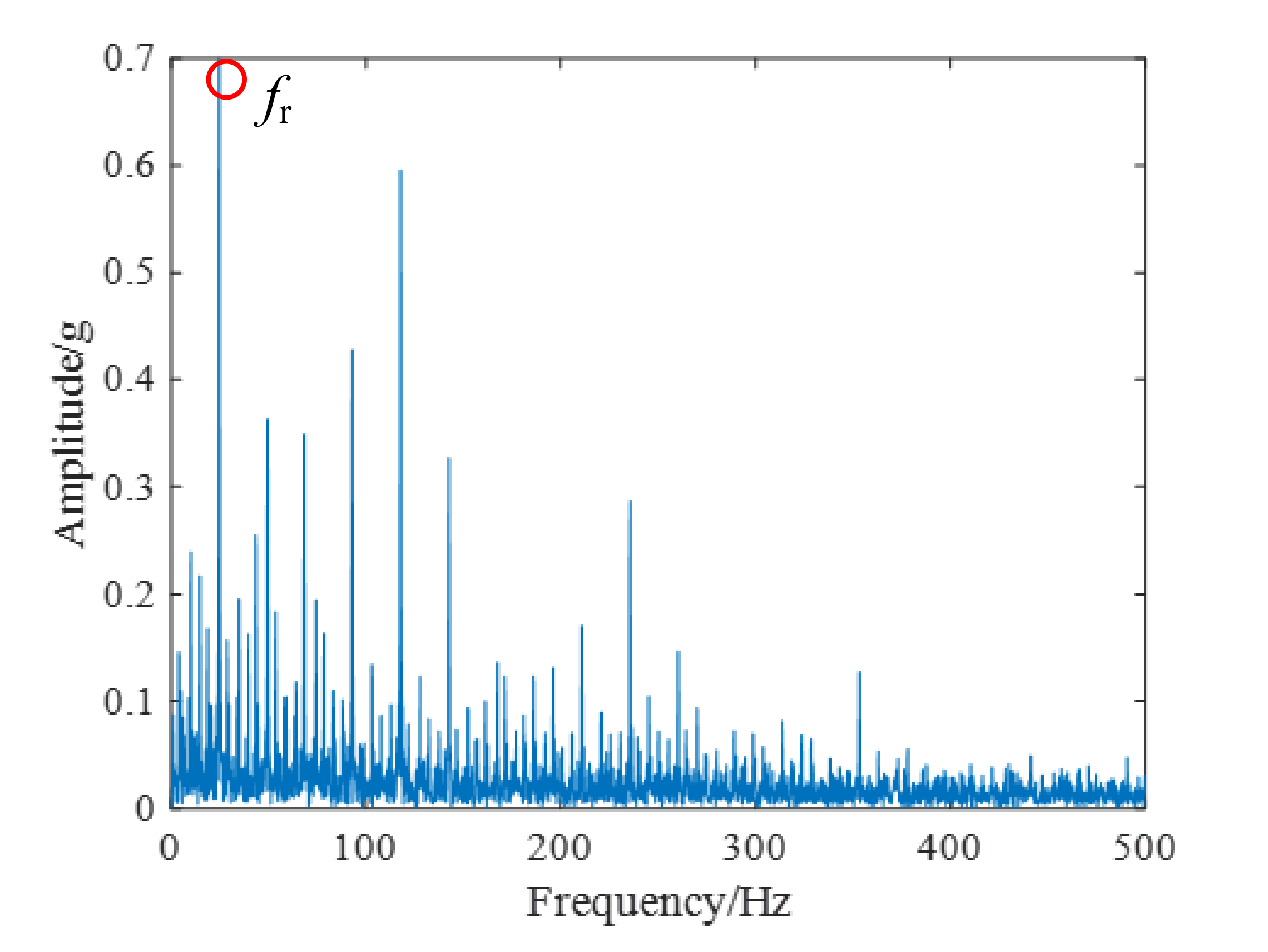
The input shaft rotational frequency is set as and the sampling rate is defined as 48,828 Hz for 3 s. According to the parameter of rolling bearing and the rotational frequency, the inner race fault character frequency as can be calculated. The time-domain waveform and frequency spectrum analysis result of rolling bearing is plotted in Figure 8. From Figure 8a, the distinct impulse phenomenon can be detected. However, because of the clutter and interference of spectral lines, the inner race fault character frequency still cannot be found in Figure 8b. Subsequently, the conventional envelope spectrum analysis is used to analyze rolling bearing signal and the outcome is shown in Figure 9. Nevertheless, only the peak corresponding to the rotational frequency can be determined, which has been marked by red circle. The above analysis results demonstrate that the common one-dimensional signal processing method cannot effectively identify the fault characteristics under the background of strong noise.
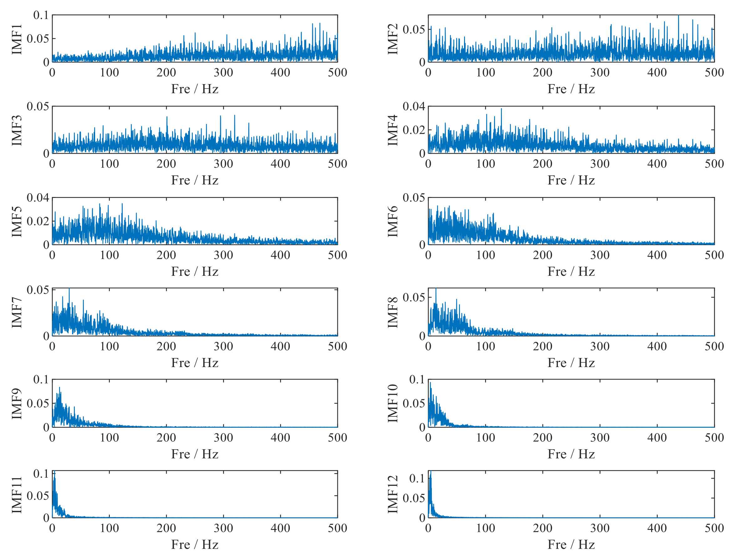
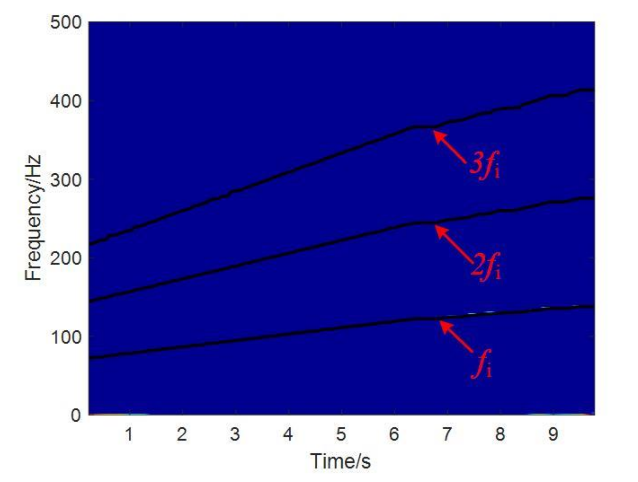
Immediately following the above analysis, the TF analysis method is conducted to undertake rolling bearing vibration signal analysis. The TF representations generated by STFT and the proposed method using RV are presented in Figure 10 and Figure 11, respectively. Since the STFT can be recognized as the Fourier transform in the short window, the TF resolution of real vibration signal is low, and the TF energy is not concentrated enough. Based on the TF denoising approach and reassignment vector, the proposed method is used to illustrate it. In accordance with Figure 11, the rotational frequency , inner race fault character frequency and its double frequency can be detected. Then, the classical EMD method is performed to analyze vibration signal and the result is drawn in Figure 12. Unfortunately, the feature frequency with inner fault cannot be found in different mode functions.
4.2. Case.2 Application to Time-varying Feature Extraction of Bearing
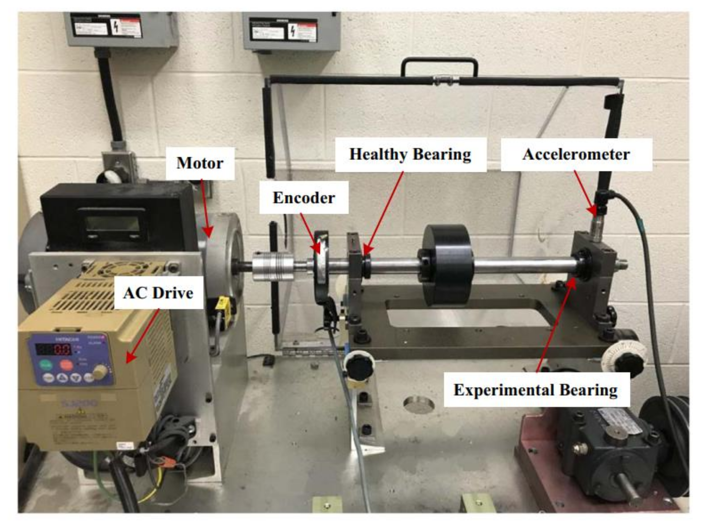
The experimental data are collected from the rolling bearing fault simulation bench on the Spectra Quest machinery fault simulator (MFS-PK5M) [34,35], and the whole device is driven by a variable frequency speed-regulating motor, as shown in Figure 13. The test bench mainly includes tachometers, the drive control system and the rotor-bearing system. There are two ER16 K rolling bearings at each end of the rotor. A special note is that the left bearing is in good condition while the right one is replaceable. Thus, the right one is selected as faulty bearings with inner fault. Structural parameters of the researched rolling bearing are described in Table 2. Theoretically, the Fault Characteristic Coefficient (FCC) corresponding to the outer race fault (FCCo) and the inner race fault (FCCI) can be respectively calculated as 3.57 and 5.43. To verify the effectiveness of this method in time-varying conditions, the operating rotational speed is increased from 13Hz to 25.7 Hz. Therefore, according to the rotation frequency and FCC, we can accurately calculate the fault characteristic frequency.
An ICP accelerometer (Model 623C01) is used to collect the vibration signal of the bearing housing at the experimental bearing, and the sampling frequency is set as 200 KHz. If the sampling rate is too high, it directly leads to large data volume; thus, the operation to realize the downsampling must be implemented.
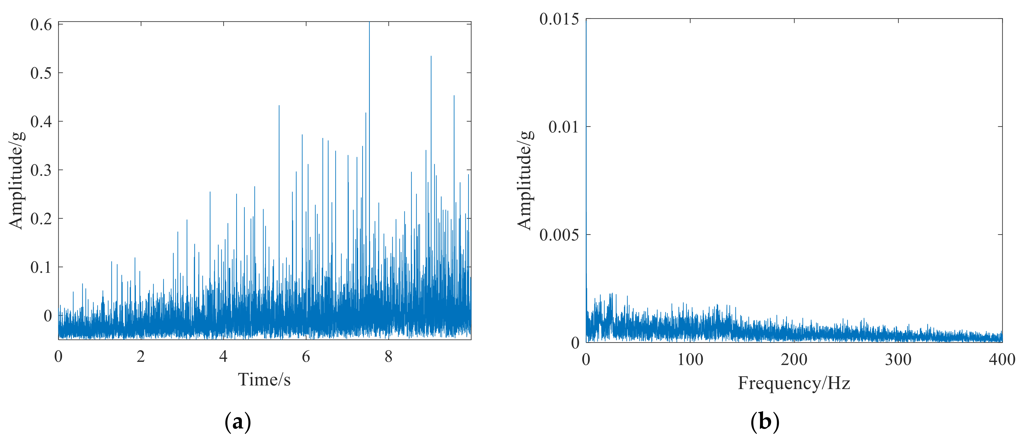
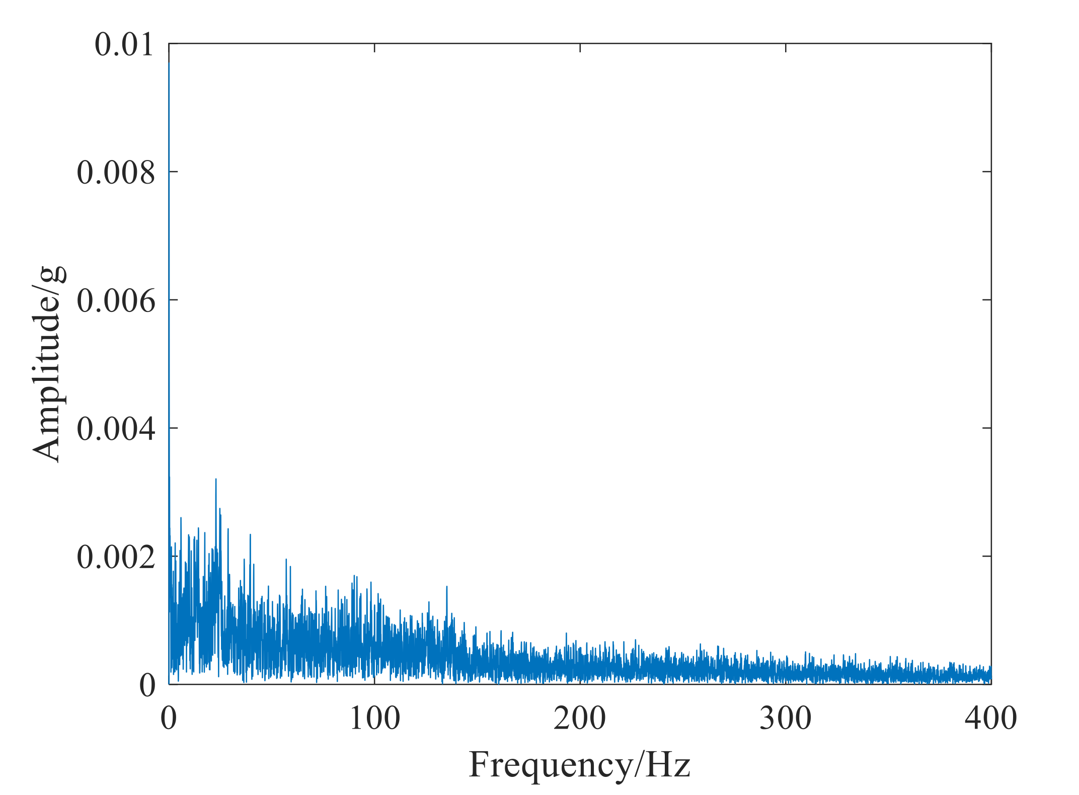
In theory, even in time-varying conditions, the fault feature can be concluded such that the inner fault characteristic frequency and its doubling components will occur in the frequency spectrum. Nevertheless, due to the change of rotational speed, the periodic impulse characteristics cannot be identified in the time domain waveform. Therefore, no matter whether it is by the time domain waveform or the spectrum analysis result described in Figure 14, the time-varying fault characteristic frequency cannot be identified. As a frequently referred vibration signal processing method, envelope spectrum analysis is performed, and its result is plotted in Figure 15. Because of the time variability and non-stationarity of the signal, however, the result is far from satisfactory.
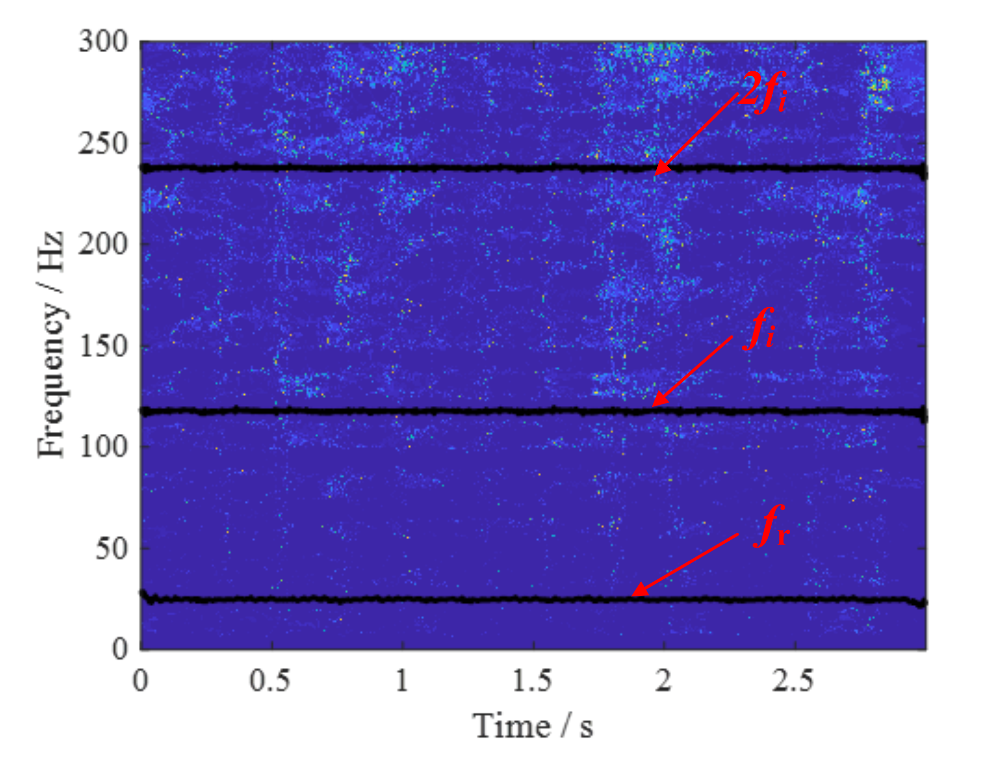
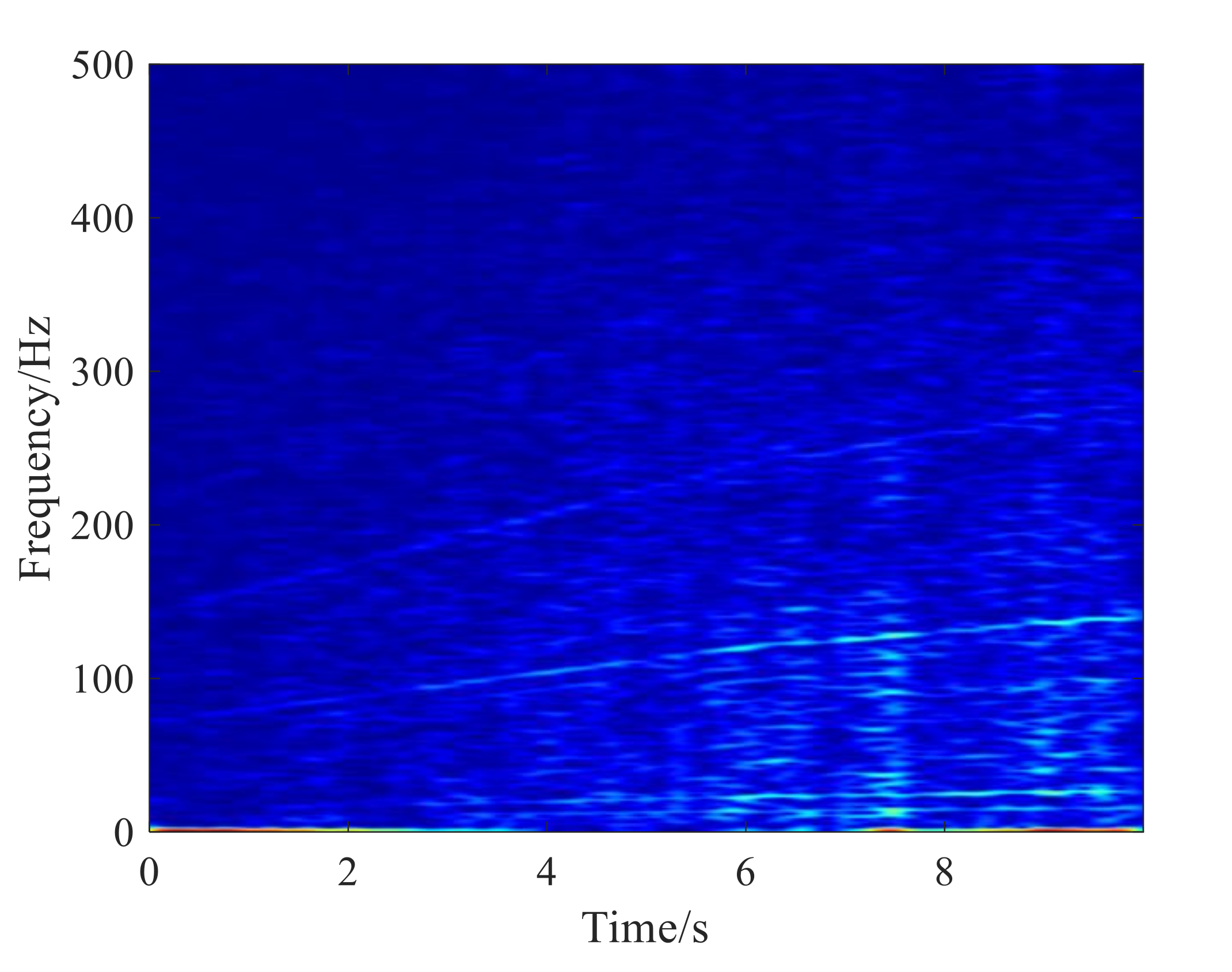
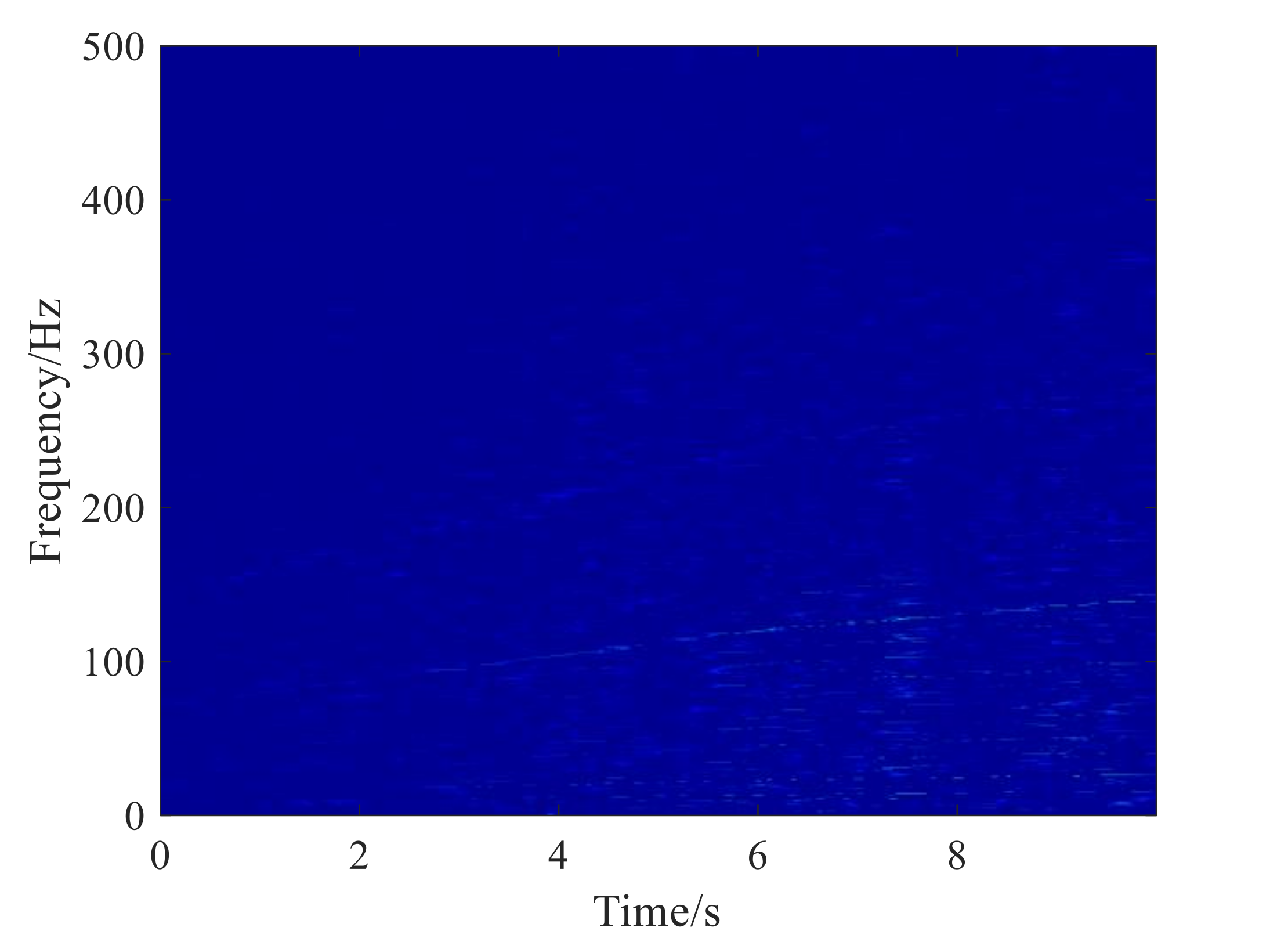
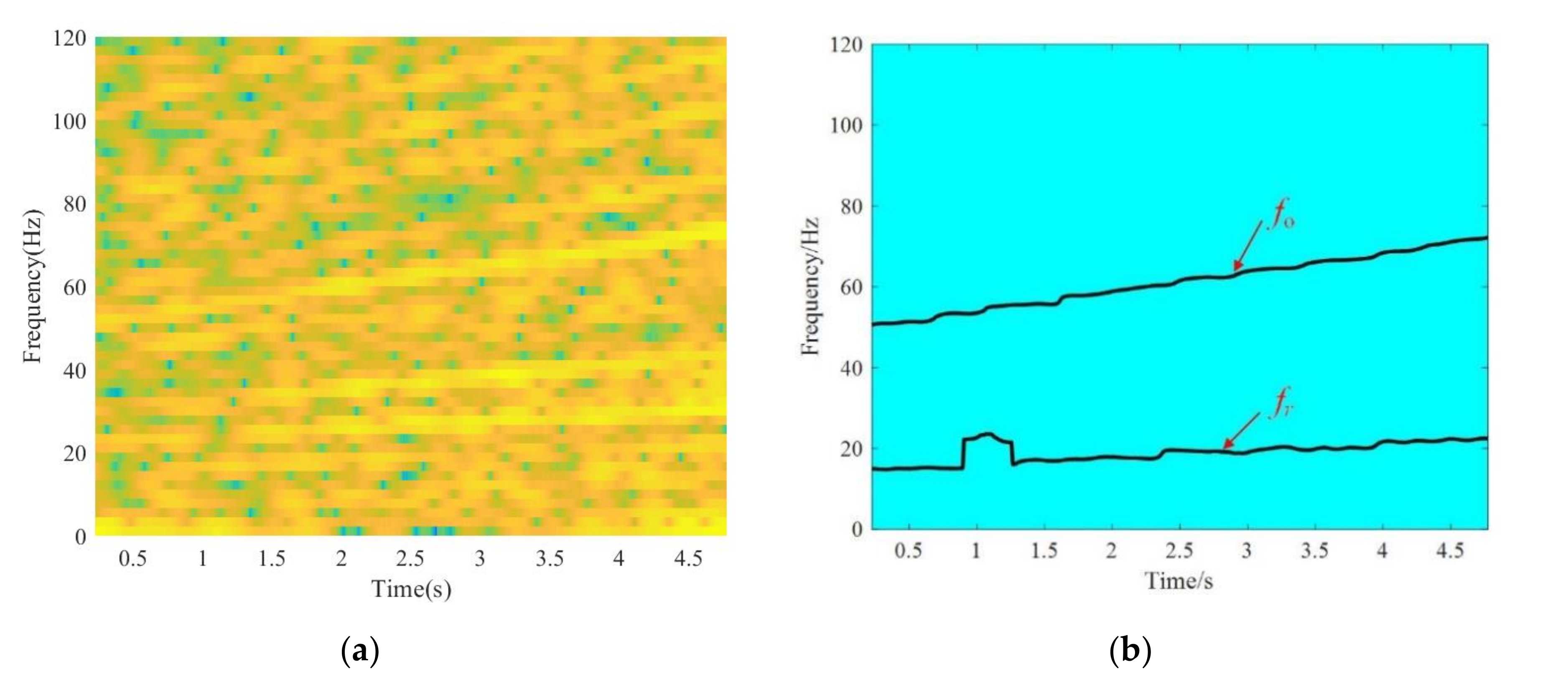
Then, the parametric time-frequency analysis methods, such as STFT and SET, are used to process the fault bearing signal for time-varying fault feature identification. Obviously, Figure 16 shows the TF analysis result generated by STFT, which has a low TF resolution. Fuzzy TF plane directly affects the readability. The main reason for this is the lack of post-processing for the TF transformation coefficient. Based on the TF reassignment framework and the classical SST theory, SET has an improvement in the performance of TF representations compared with STFT. The trend of time-varying characteristic changing can be obtained in Figure 17. However, the energy of the characteristic curve is not concentrated enough, and many independent components exist in the TF plane. Finally, the proposed method in this paper is conducted to bearing fault signal analysis and the corresponding result is drawn in Figure 18. It is evident that the proposed method based on TF denoising scheme and reassignment vector has a better performance. The time-varying rotation frequency , and can be identified in the TF plane. From this, the conclusion can be drawn that the rolling bearing has an inner fault. Meanwhile, the result provided by EMD is plotted in Figure 19 and the concerned time-varying characteristic cannot be detected. In a summary, through the analysis of rolling bearing fault data, the validity of the proposed signal decomposition algorithm from the TF plane is illustrated.
Moreover, to further illustrate the effectiveness of the proposed method in dealing with various types of faults, fault signal analysis of bearing outer race under time-varying speed in the above Spectra Quest machinery fault simulator has also been conducted. The vibration signal is measured from a faulty bearing with an outer race defect and the operating rotational frequency fr increases from 14.0 Hz to 21.7 Hz. Similarly, according to the rotation frequency fr and Fault Characteristic Coefficient (FCC), we can accurately calculate the time-varying outer race fault characteristic frequency fo [36].
Figure 20 shows the TFR obtained by STFT and the proposed method. Due to deficiency of STFT in dealing with strong frequency modulation signal (especially in the noisy environment), time-frequency blurs occur in the result generated by STFT in Figure 20a. Fortunately, the proposed method has suggested higher resolution of ridges, compared with STFT in time-frequency plane in Figure 20b. The varied rotational frequency fr and outer race fault characteristic frequency fo can both be identified in the TF plane. Therefore, we can diagnose the outer race fault, which is consistent with the actual situation. Based on the above analysis, we can make a conclusion that the method presented in this paper is effective at diagnosing fault signals of bearing inner race and outer race.
5. Conclusions
Aiming at feature extraction and identification of multi-component signals in mechanical equipment fault diagnosis, an adaptive signal decomposition algorithm derived from Rearrangement Vector (RV) is proposed in this paper. The main research work of this paper is summarized as follows: (1) The TF denoising operation is primarily considered by sparse low-rank matrix estimation under the convex optimization scheme. Through non-convex penalty function and ADMM algorithm, the desired TF transformation coefficient matrix is obtained. (2) Based on the outcome, RV is employed to identify TF signature in the two-dimensional TF plane, which concerns different ridge curves and model components. Thus, adaptive mode decomposition can be implemented by RV. (3) Combining the advantage of TF denoising approach and RV action in TF plane, the proposed method has been successfully applied to bearing fault diagnosis. Whether rolling bearing fault analysis is under stationary condition or time-varying condition, the results show that the method proposed in this paper is of obvious engineering application value.
Author Contributions
C.Y. and X.W. provided the research ideas and the theoretical analysis, wrote the code and the paper. C.Y., Y.Z. and W.K. designed the experiment, collected the experiment data and analyzed the data. C.Y. and X.W. verified the data, sorted out the graphs and the chart as well as the related literature. All authors have read and agreed to the published version of the manuscript.
Funding
This research was funded by National Natural Science Foundation of China grant number 51805382, Lishui public welfare technology application and research project grant number 2019GYX03, and Zhejiang Provincial Market Supervision System Research Project grant number 20190357.
Conflicts of Interest
The authors claim that there is no conflict of interests regarding the publication of this article.
References
- Jerome, A.; Julien, G.; Hugo, A. Feedback on the surveillance 8 challenge: Vibration-based diagnosis of a safran aircraft engine. Mech. Syst. Signal Process. 2017, 97, 112–114. [Google Scholar]
- Milos, B.; Vesna, P.B. Post-processing of time-frequency representations in instantaneous frequency estimation based on ant colony optimization. Signal Process. 2017, 138, 195–210. [Google Scholar]
- Feng, Z.; Chen, X.; Wang, T. Time-varying demodulation analysis for rolling bearing fault diagnosis under variable speed conditions. J. Sound Vib. 2017, 400, 71–85. [Google Scholar] [CrossRef]
- Auger, F.; Flandrin, P.; Lin, Y.; McLaughlin, S.; Meignen, S.; Oberlin, T.; Wu, H. Time-frequency reassignment and synchrosqueezing: An overview. IEEE Signal Process. Mag. 2013, 30, 32–41. [Google Scholar] [CrossRef] [Green Version]
- Auger, F.; Flandrin, P. Improving the readability of time-frequency and time-scale representations by the reassignment method. IEEE Signal Process. Mag. 1995, 43, 1068–1089. [Google Scholar] [CrossRef] [Green Version]
- Guo, X.; Chen, L.; Shen, C. Hierarchical adaptive deep convolution neural network and its application to bearing fault diagnosis. Measurement 2016, 93, 490–502. [Google Scholar] [CrossRef]
- Ghoreishi, S.F.; Imani, M. Offline fault detection in gene regulatory networks using next-generation sequencing data. In Proceedings of the 2019 53rd Asilomar Conference on Signals, Systems, and Computers, Pacific Grove, CA, USA, 3–6 November 2019; pp. 1344–1348. [Google Scholar]
- Mahdi, I.; Edward, D. Boolean Kalman Filter and Smoother Under Model Uncertainty. Automatica 2020, 111, 108609. [Google Scholar]
- He, D.; Cao, H.; Wang, S.; Chen, X. Time-reassigned synchrosqueezing transform: The algorithm and its applications in mechanical signal processing. Mech. Syst. Signal Process. 2019, 117, 255–279. [Google Scholar] [CrossRef]
- Roehri, N.; Lina, J.; Mosher, J.C.; Bartolomei, F.; Benar, C. Time-Frequency Strategies for Increasing High-Frequency Oscillation Detectability in Intracerebral EEG. IEEE Trans Bio. Med. Eng 2016, 63, 2595–2606. [Google Scholar] [CrossRef] [Green Version]
- Kiran, G.; Parimalasundar, E.; Elangovan, D.; Sanjeevikumar, P.; Lannuzzo, F.; Holm-Nielsen, J.B. Fault Investigation in Cascaded H-Bridge Multilevel Inverter through Fast Fourier Transform and Artificial Neural Network Approach. Energies 2020, 13, 1299. [Google Scholar] [CrossRef] [Green Version]
- Shalu, C.; Sachin, T.; Varun, B. A flexible analytic wavelet transform based approach for motor-imagery tasks classification in BCI applications. Comput. Methods Programs Biomed. 2020, 187, 105–325. [Google Scholar]
- Yi, C.; Lv, Y.; Dang, Z. Quaternion singular spectrum analysis using convex optimization and its application to fault diagnosis of rolling bearing. Measurement 2017, 103, 321–332. [Google Scholar] [CrossRef]
- Meignen, S.; Pham, D. Retrieval of the Modes of Multicomponent Signals From Downsampled Short-Time Fourier Transform. IEEE Signal. Process. 2018, 66, 6204–6215. [Google Scholar] [CrossRef] [Green Version]
- Wang, Y.; Rao, Y.; Xu, D. Multichannel maximum-entropy method for the Wigner-Ville distribution. Geophysics 2020, 85, 25–31. [Google Scholar] [CrossRef]
- Li, L.; Cai, H.; Han, H.; Jiang, Q.; Ji, H. Adaptive short-time Fourier transform and synchrosqueezing transform for non-stationary signal separation. IEEE Signal. Process. 2020, 166, 107231. [Google Scholar] [CrossRef]
- Yi, C.; Lv, Y.; Xiao, H.; Huang, T.; You, G. Multisensor signal denoising based on matching synchrosqueezing wavelet transform for mechanical fault condition assessment. Meas. Sci. Technol. 2018, 29, 45104. [Google Scholar] [CrossRef]
- Zhou, P.; Dong, X.; Chen, S. Parameterized Model Based Short-time Chirp Component Decomposition. Signal Process. 2018, 145, 146–154. [Google Scholar] [CrossRef]
- Daubechies, I.; Lu, J.; Wu, H. Synchrosqueezed wavelet transforms: An empirical mode decomposition-like tool. Appl. Comput. Harmon. A 2011, 30, 243–261. [Google Scholar] [CrossRef] [Green Version]
- Yu, G.; Yu, M.; Xu, C. Synchroextracting Transform. IEEE Ind. Electron. 2017, 64, 8042–8054. [Google Scholar] [CrossRef]
- Oberlin, T.; Meignen, S.; Perrier, V. Second-Order Synchrosqueezing Transform or Invertible Reassignment? Towards Ideal Time-Frequency Representations. IEEE Signal Process. 2015, 63, 1335–1344. [Google Scholar] [CrossRef] [Green Version]
- Moghadasian, S.S.; Gazor, S. Sparsely Localized Time-Frequency Energy Distributions for Multi-Component LFM Signals. IEEE Signal Process. 2020, 27, 6–10. [Google Scholar] [CrossRef]
- Yu, G. A geometry study on reassignment method and synchrosqueezing transform. In Proceedings of the 2018 Chinese Automation Congress (CAC), Xian, China, 30 November–2 December 2018; IEEE: Picataway, NJ, USA, 2019. [Google Scholar]
- Bruni, V.; Tartaglione, M.; Vitulano, D. A Fast and Robust Spectrogram Reassignment Method. Mathematics 2019, 7, 358. [Google Scholar] [CrossRef] [Green Version]
- Pham, D.; Meignen, S. An Adaptive Computation of Contour Representations for Mode Decomposition. IEEE Signal Process. 2017, 24, 1596–1600. [Google Scholar] [CrossRef] [Green Version]
- Meignen, S.; Oberlin, T.; Depalle, P.; Flandrin, P.; McLaughlin, S. Adaptive multimode signal reconstruction from time–frequency representations. Philos. Trans. R. Soc. A Math. Phys. Eng. Sci. 2016, 374, 201–205. [Google Scholar] [CrossRef] [Green Version]
- Yi, C.; Lv, Y.; Xiao, H.; You, G.; Dang, Z. Research on the Blind Source Separation Method Based on Regenerated Phase-Shifted Sinusoid-Assisted EMD and Its Application in Diagnosing Rolling-Bearing Faults. Appl. Sci. 2017, 7, 414. [Google Scholar] [CrossRef]
- Chen, X.; Yang, Y.; Cui, Z.; Shen, J. Vibration fault diagnosis of wind turbines based on variational mode decomposition and energy entropy. Energy 2019, 174, 1100–1109. [Google Scholar] [CrossRef]
- Ding, Y.; He, W.; Chen, B.; Zi, Y.; Selesnick, I.W. Detection of faults in rotating machinery using periodic time-frequency sparsity. J. Sound Vib. 2016, 382, 357–378. [Google Scholar] [CrossRef] [Green Version]
- Parekh, A.; Selesnick, I.W. Enhanced Low-Rank Matrix Approximation. IEEE Signal Process. 2016, 23, 493–497. [Google Scholar] [CrossRef]
- Parekh, A.; Selesnick, I.W. Improved sparse low-rank matrix estimation. IEEE Signal Process. 2017, 139, 62–69. [Google Scholar] [CrossRef] [Green Version]
- Giselsson, P.; Boyd, S. Linear Convergence and Metric Selection in Douglas-Rachford Splitting and ADMM. IEEE Trans. Autom. Control 2016, 62, 532–544. [Google Scholar] [CrossRef] [Green Version]
- Bechhoefer, E. A Quick Introduction to Bearing Envelope Analysis, MFPT Data. Available online: http://www.mfpt.org/FaultData/FaultData.htm.Set (accessed on 10 March 2020).
- Huang, H.; Baddour, N.; Liang, M. Multiple time-frequency curve extraction Matlab code and its application to automatic bearing fault diagnosis under time-varying speed conditions. Methods X 2019, 6, 1415–1432. [Google Scholar] [CrossRef] [PubMed]
- Huang, H.; Baddour, N. Bearing vibration data collected under time-varying rotational speed conditions. Data Brief 2018, 21, 1745–1749. [Google Scholar] [CrossRef] [PubMed]
- Antoni, J.; Randall, B.R. A Stochastic Model for Simulation and Diagnostics of Rolling Element Bearings with Localized Faults. J. Vib. Acoust. 2003, 125, 282–289. [Google Scholar] [CrossRef]
Figure 1.
The flowchart of the proposed method.

Figure 2.
The researched numerical simulation signal. (a) Numerical signal shown in time-domain. (b) Numerical signal shown in frequency-domain.
Figure 2.
The researched numerical simulation signal. (a) Numerical signal shown in time-domain. (b) Numerical signal shown in frequency-domain.

Figure 3.
The TFR obtained by short-time Fourier transform (STFT) and reassignment vector (RV) method. (a) TFR obtained by STFT. (b) TFR obtained by the proposed method.
Figure 3.
The TFR obtained by short-time Fourier transform (STFT) and reassignment vector (RV) method. (a) TFR obtained by STFT. (b) TFR obtained by the proposed method.

Figure 4.
The time-frequency (TF) mode decomposition by the proposed method.

Figure 5.
Performance of signal decomposition and reconstruction by proposed method. (a) multi-components signal decomposition. (b) signal reconstruction.
Figure 5.
Performance of signal decomposition and reconstruction by proposed method. (a) multi-components signal decomposition. (b) signal reconstruction.

Figure 6.
Performance of signal decomposition by Empirical Mode Decomposition (EMD).

Figure 7.
The rolling bearing with inner race fault.

Figure 8.
The rolling bearing vibration signal shown in time and frequency domain. (a) the time-domain waveform of the bearing signal. (b) the frequency-domain waveform of the bearing signal.
Figure 8.
The rolling bearing vibration signal shown in time and frequency domain. (a) the time-domain waveform of the bearing signal. (b) the frequency-domain waveform of the bearing signal.

Figure 9.
The envelope spectrum analysis results.

Figure 10.
The TFR generated by STFT.

Figure 11.
The result provided by proposed method using RV.

Figure 12.
The result provided by EMD.

Figure 13.
Experimental equipment.

Figure 14.
The time-domain and frequency-domain waveform of original bearing signal. (a) the time-domain waveform. (b) the frequency spectrum analysis result.
Figure 14.
The time-domain and frequency-domain waveform of original bearing signal. (a) the time-domain waveform. (b) the frequency spectrum analysis result.

Figure 15.
The envelope spectrum analysis results.

Figure 16.
The result provided by STFT.

Figure 17.
The result provided by Synchroextracting Transform (SET).

Figure 18.
The result provided by the proposed method using RV.

Figure 19.
The result provided by EMD.

Figure 20.
TFR of bearing outer race fault signal generated by different methods. (a) TFR generated by STFT. (b) the result provided by proposed method.
Figure 20.
TFR of bearing outer race fault signal generated by different methods. (a) TFR generated by STFT. (b) the result provided by proposed method.


Table 1.
The structure parameter of rolling bearing.
| Roller Diameter | Pitch Diameter | Number of Elements | Contact Angle | Load/lbs |
|---|---|---|---|---|
| 0.235 | 1.245 | 8 | 0 | 300 |
Table 2.
Parameters of rolling bearing.
| Bearing Type | Pitch Diameter | Ball Diameter | Number of Balls | FCCI | FCCO |
|---|---|---|---|---|---|
| ER16K | 38.52 mm | 7.94 mm | 9 | 5.43 | 3.57 |
© 2020 by the authors. Licensee MDPI, Basel, Switzerland. This article is an open access article distributed under the terms and conditions of the Creative Commons Attribution (CC BY) license (http://creativecommons.org/licenses/by/4.0/).
Share and Cite
MDPI and ACS Style
Yi, C.; Wang, X.; Zhu, Y.; Ke, W. A Novel Adaptive Mode Decomposition Method Based on Reassignment Vector and Its Application to Fault Diagnosis of Rolling Bearing. Appl. Sci. 2020, 10, 5479. https://doi.org/10.3390/app10165479
AMA Style
Yi C, Wang X, Zhu Y, Ke W. A Novel Adaptive Mode Decomposition Method Based on Reassignment Vector and Its Application to Fault Diagnosis of Rolling Bearing. Applied Sciences. 2020; 10(16):5479. https://doi.org/10.3390/app10165479
Chicago/Turabian StyleYi, Cancan, Xing Wang, Yajun Zhu, and Wei Ke. 2020. "A Novel Adaptive Mode Decomposition Method Based on Reassignment Vector and Its Application to Fault Diagnosis of Rolling Bearing" Applied Sciences 10, no. 16: 5479. https://doi.org/10.3390/app10165479
Note that from the first issue of 2016, this journal uses article numbers instead of page numbers. See further details here.