Hybridizing Deep Learning and Neuroevolution: Application to the Spanish Short-Term Electric Energy Consumption Forecasting

Abstract

The electric energy production would be much more efficient if accurate estimations of the future demand were available, since these would allow allocating only the resources needed for the production of the right amount of energy required. With this motivation in mind, we propose a strategy, based on neuroevolution, that can be used to this aim. Our proposal uses a genetic algorithm in order to find a sub-optimal set of hyper-parameters for configuring a deep neural network, which can then be used for obtaining the forecasting. Such a strategy is justified by the observation that the performances achieved by deep neural networks are strongly dependent on the right setting of the hyper-parameters, and genetic algorithms have shown excellent search capabilities in huge search spaces. Moreover, we base our proposal on a distributed computing platform, which allows its use on a large time-series. In order to assess the performances of our approach, we have applied it to a large dataset, related to the electric energy consumption registered in Spain over almost 10 years. Experimental results confirm the validity of our proposal since it outperforms all other forecasting techniques to which it has been compared.

1. Introduction

The electric energy needs are constantly growing. It is estimated that such demand will increment from 549 quadrillion British thermal unit (Btu), registered in 2012, to 629 quadrillion Btu in 2020. A further increment of $48\%$ is estimated by 2040 [1].

The accurate estimation of the short-term electric energy demand provides several benefits. The economic benefits are evident because this would allow us to allocate only the right amount of resources that are needed in order to produce the amount of energy actually needed to face the actual demand [2,3]. There are also environmental aspects to consider, since, by producing only the right amount of energy required, the emission of $C{O}_2$ would be reduced as well. In fact, energy efficiency is another relevant goal pursued with these kinds of approaches since the accurate forecasting of electricity demand in public buildings or in industrial plants usually leads to energy savings [4,5,6].

Such observations highlight the importance of being able to count on efficient electric energy management systems and prediction strategies and, consequently, different organizations around the world are taking actions in order to increase energy efficiency. Hence, the European Union (EU), under the current energy plan [7], established that EU countries will have to embrace various energy efficiency requirements with the objective of improving at least a $20\%$ the energy efficiency. In addition to this, countries belonging to the EU closed an agreement to obtain an additional $27\%$ increment of the efficiency by 2020, with the possibility of increasing the target to $30\%$ by the year 2030.

Forecasting algorithms could contribute to reaching such objectives [2,3]. In this context, energy demand forecasting can be described as the problem of predicting the energy demand within a specified prediction horizon, using past data, or, in other words, a historical window.

Depending on the time scale of the predictions, we can generally distinguish three classes of forecasting, i.e., short, medium and long-term forecasting. In short-term forecasting, the objective is to predict the energy demand using horizons going from one hour up to a week. If the prediction horizon is set between one week and one month, we talk about medium-term forecasting, while long-term forecasting involves longer horizons [8].

In this paper, we focus on the problem of short-term forecasting. This is an important problem, since with accurate predictions of short-term load it would be possible to make precisely plan the resources that need to be allocated in order to face the actual demand, which, as already stated, would have benefits from both the economical and environmental points of view.

To this aim, we propose an extension of the work proposed in [9], where a deep feed-forward neural network was used to tackle the short-term load forecasting problem. In the original work, the tools provided by the H2O big data analysis framework were used along with the Apache Spark platform for distributed computing.

Differently from [9], where a grid search strategy was used for setting the values of the deep neural network parameters, in this work, we propose to use a genetic algorithm (GA) in order to determine a sub-optimal set of hyper-parameters for building the deep neural network that will then be used for obtaining the predictions. Due to the large search space composed of all hyper-parameters of a deep learning network, and considering that the method should be scalable for big data environments, it has been decided to reduce the search range of the GA. For this reason, our proposal will not always be able to find the optimal set of hyper-parameters for the network, but ensures a competitive sub-optimal configuration.

Our main motivation lies in the observation that the success of deep learning depends on finding an architecture to fit the task. As deep learning has scaled up to more challenging problems, the architectures have become difficult to design by hand [10]. To this aim, evolutionary algorithms (EAs) can be used in order to find good configurations of the deep neural networks. Individuals can be set of parameter values, and their fitnesses are determined based on how well they can be trained to perform in the task.

This field is known as neuroevolution, which, in a nutshell, can be defined as a strategy for evolving neural networks with the use of EAs [11]. Usually, deep artificial neural networks (DNNs) are trained via gradient-based learning algorithms, namely backpropagation, see for example [12]. EAs can be used in order to seek the optimal values of hyper parameters, for the example the learning rates, or the number of layers and the amount of neurons per layer, among others.

It has been proven that EAs can be combined with backpropagation-based techniques, such as Q-learning and policy gradients, on difficult problems, see, e.g., [13]. In fact, the problem of setting parameters for such methods is not trivial, and, if the parameters are not correctly set, the forecasting can be poor.

The above observations motivate us to use a neuroevoltution approach in order to tackle the short-term energy load forecasting problem. In order to validate our proposal, we applied it to a dataset regarding the electric energy consumption registered over almost 10 years in Spain. We have also compared our proposal with other standard and machine learning (ML) strategies, and results obtained confirm that our proposal achieves the best predictions.

In the following, we summarise the main contributions of this paper:

• We propose a new general-purpose approach based on deep learning for big data time-series forecasting. Due to the high computational cost of the deep learning, we adopted a distributed computing solution in order to be able to process large time series.
• The hyper-parameter tuning and optimization of the deep neural networks is a key factor for obtaining competitive results. Usually, the hyper-parameters of a deep neural network are pre-fixed previously or computed by a grid search, which performs an exhaustive search through the whole set of established hyper-parameters. However, the grid search presents an important limitation: it works with discrete values, which greatly limits the fine-tuning of the vast majority of hyper-parameters. Thus, an evolutionary search is proposed to find the hyper-parameters.
• We conduct a wide experimentation using Spanish electricity consumption registered over 10 years, with measurements recorded every 10 min. Results show a mean relative error of 1.44%, demonstrating the high potential of the proposed approach, also compared to other forecasting strategies.
• We evaluate our proposal predictive accuracy and compare it with a strategy based on deep learning using a grid search for setting the hyper parameters. The evolutionary search showed to be effective in order to achieve higher accuracy.
• In addition, we compare the approach with seven state-of-the-art forecasting algorithms such as ARIMA, decision tree, an algorithm based on gradient boosting, random forest, evolutionary decision trees, a standard neural network and an ensemble proposed in [14], outperforming all of them.
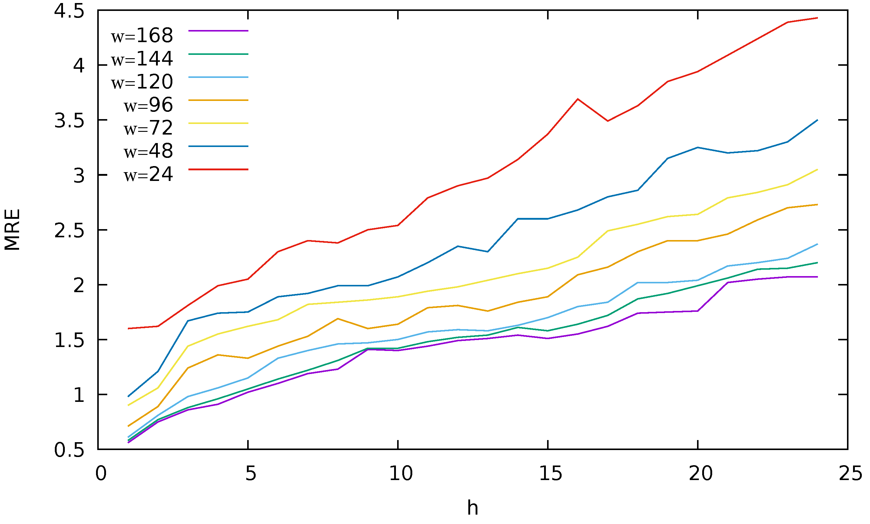
• We analyze how the size of the historical window affects the accuracy of the model. We found that when using the past 168 values as input features to predict the next 24 values the best results were obtained.

The rest of the paper is organized as follows. In Section 2 we provide a brief overview of the state of the art of electric energy time-series forecasting. The dataset used in this work is described and analyzed in Section 3.1, while the methodology used is discussed in Section 3.2. In Section 4 we describe the results obtained by our approach and compare them to those achieved by other strategies. Finally, we draw the main conclusions and identify futures works in Section 5.

2. Related Works

As previously mentioned, a lot of attention has been paid to short-term electricity consumption forecasting during the last decades. This section provides a brief overview of up-to-date related works.

We can distinguish two main strategies to predict energy consumption. A first strategy is based on conventional methods, e.g., [15,16], whilst an alternative, and more recent strategy, is based on ML techniques.

Conventional methods include, among others, statistical analysis, smoothing techniques such as the autoregressive integrated moving average (ARIMA), exponential smoothing and regression-based approaches. Such techniques can obtain satisfactory results when applied to linear problems.

In contrast, ML strategies are also suitable for non-linear cases. We refer the reader to [17] for an expanded survey on data mining techniques applied to electricity-related time-series forecasting. In this work, several markets and prediction horizons are considered and discussed.

Popular ML techniques successfully applied to the forecasting of power consumption data include Artificial Neural Networks (ANN) [18,19,20] or Support Vector Machines (SVM), see, for instance, [21,22].

Other strategies are based on pattern similarity [23,24]. Since 2011, when the Pattern Sequence based Forecasting (PSF) algorithm was published [24], a number of variants has been proposed for forecasting this kind of time-series [25,26,27,28], including an R package [29] and a big data version [30]. Grey forecast models have also been used for predicting time-series. In particular such an approach has been applied to forecast the demand of natural gas in China. For instance, in [31] a self-adapting intelligent grey prediction model was proposed, where a linear function was used in order to automatically optimize the parameters used by the proposed grey model. This strategy was substituted with a genetic algorithm in [32], which resolved various limitations of the previous mechanism. A novel time-delayed polynomial grey model was introduced in [33], while in [34] authors proposed a least squares support vector machine model based on grey analysis.

Recently, Deep Learning (DL) has also been applied to this problem, see, e.g., [9,35]. However, to the best of our knowledge, a part from the early version [36] and few other works, such as [37], in which Brazilian data were analyzed, or [38] for Irish data, or [39] for Chinese data, no other works based on DL can be found in the literature.

Although ML techniques provide effective solutions for time-series forecasting, these methods tend to get stuck in a local optimum. For instance, ANN and SVM may get trapped in a local optimum if their configuration parameters are not properly set.

Recently, methods developed for big data environments have also been applied to electricity consumption forecasting. In [40] an approach based on the k-weighted nearest neighbours algorithm was introduced and implemented using the Apache Spark framework. The performances of the resulting algorithm were tested using a Spanish energy consumption Big Data time-series. As mentioned above, in 2018, Torres et al. [9] proposed a DL model to deal with big data time-series forecasting. In particular, the H2O Big Data analysis framework was used. Results from a real-world dataset composed of electricity consumption in Spain, with a ten-minute frequency sampling rate, from 2007 to 2016 were reported.

As can be seen, although much attention has been paid to the electricity consumption forecasting problem, few works based on DL have been proposed. Moreover, such existing works did not applied any metaheuristic strategy to set the parameters. These facts highlight the existing gap in the literature and justify, from the authors’ point of view, the development of this work.

As previously stated, in this paper we aim at using DL, in order to perform time-series forecasting. In DL, many parameters have to be set. The setting of such parameters have a great influence on the final results obtained by such a strategy. An alternative way to set the DL parameters is to use an Evolutionary Algorithm (EA) in order to find a sub-optimal set of parameters. This field, known as neuroevolution [11,41], has received much attention lately in the ML community. Neuroevolution enables important capabilities such as learning neural network building blocks, e.g., the activation function, hyperparameters, architectures and even the algorithms for learning themselves. Neuroevolution also differs from DL (and deep reinforcement learning) since in neuroevolution a population of solutions is maintained during the search. This provides extreme exploration capabilities and the possibility of massive parallelization. There also exist alternative strategies in order to find an optimal set of parameter, going from grid search to more complex approaches, such as methods based on Bayesian optimization, see, for instance [42,43]. Neuroevolution has been successfully applied to different fields, especially in image classification, where Convolutional Neural Networks (CNN) are evolved, see, for instance [44,45,46,47]. To be best of our knowledge, Neuroevolution has not been applied to time-series forecasting.

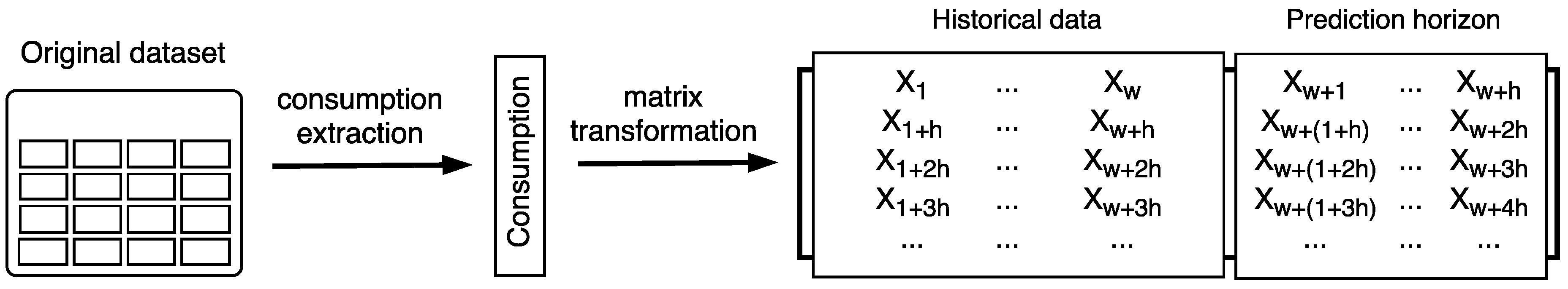
3. Data and Methodology

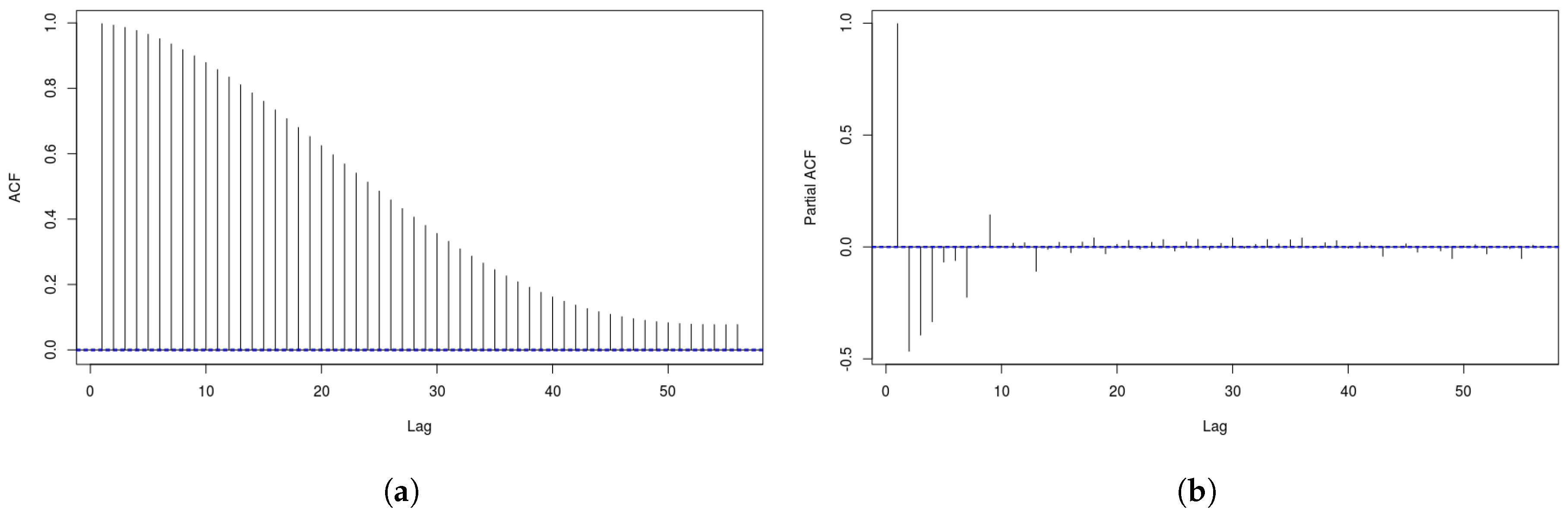
3.1. Data

In order to assess the quality of our proposal, we used a dataset containing information regarding the global electricity consumption registered in Spain (in MW), available at [48].

In particular, the data were recorder over a period going from 1 January 2007 at midnight until 21 June 2016 at 11:40 pm, which amounts to nine years and six months. Specifically, the data is relative to the consumption measured at 10 minutes intervals, meaning that the dataset consists of a total of 497,832 measurements. No missing values or outliers were found, since data are provided by the Spanish Nominated Electricity Market Operator (NEMO) and all data are already preprocessed and cleaned.

Time-series regarding the electric energy demand are typically non-stationary. This fact renders the problem of forecasting the electric energy demand challenging, since such time-series present statistical properties, such as the mean, variance and autocorrelation, that are not all constant over time. It follows that they can present changes in variance, trends or seasonal effects. For this reason, we performed a preliminary study of the dataset in order to assess whether or not the time-series used in this paper is stationary. To this aim, we analyzed the AutoCorrelation Function (ACF) and the Partial AutoCorrelation Function (PACF) of the time-series, which are reported in Figure 1.

From Figure 1a, we can notice that the time-series has a high correlation with a number significant of lags, while from Figure 1b we can see that there are four spikes in the first lags, from which we can determine the order of autoregression of the time-series. From these observations, we can conclude that the time-series is not stationary, and that the order of autoregression to be used should be 4.

A preprocessing of the dataset had to be applied before it could be used. In particular, we used the preprocessing strategy proposed in [36], which is graphically depicted in Figure 2. In a first step, we extract the attribute corresponding to the energy consumption, obtaining in this way a consumption vector $V_c$.

From $V_c$ matrix $M_c$ is built. The size of $M_c$ depends on the values of the historical window (w) and of the prediction horizon (h) used. Notice that w determines the number of previous entries that will be used in order to induce a forecasting model that will be used to estimate the subsequent h values.

In this work, as in [36], h was set to 4 hours, which corresponds to a value of 24 reads. Various values of w were tested.

In particular, w was set to values 24, 48, 72, 96, 120, 144 and 168. Such values correspond to 4, 8, 12, 16, 20, 24 and 28 hours, respectively.

One the matrix $M_c$ has been obtained, we divided the resulting dataset into a $70\%$ used as a training set, while the remaining $30\%$ was used as a testing set. This means that the prediction model was obtained using only the training set. The forecasting performances of the so induced model are assessed on the test set, which basically represents unseen data. Within the training set, a $30\%$ is used as a validation set for determining the deep learning hyperparameters.

These preprocessing steps yield the generation of seven different matrices, whose information is reported in

Table 1. Dataset information depending on the value of w.

w	#Rows	#Columns	File Size (In MB)
24	20,742	48	6
48	20,741	72	9
72	20,740	96	11.9
96	20,739	120	14.9
120	20,738	144	17.9
144	20,737	168	20.9
168	20,736	192	23.9

. Note that for all the obtained datasets, the last 24 columns represent the prediction horizon.

3.2. Methodology

This section describes the proposed methodology for forecasting time-series using a deep learning approach. There are various deep learning architectures which can be used for time-series forecast, such as convolutional neural nets (CNN), recurrent neural nets (RNN) or feed-forward neural nets (FFNN).

In this paper, a deep feed-forward network has been used, implemented by R package H2O [49]. H2O is an open-source framework that implements various machine learning techniques in a parallel and distributed way using a single machine or a cluster of machines, being scalable for big data projects.

Among the algorithms included in H2O, we can find a feed-forward neural network, that is the most common network architectures. The main characteristic of this net is that each neuron is a basic element of processing and their information is propagated through adjacent neurons.

In addition, in order to select the configuration of the network hyperparameters, we used a GA, which was implemented by using the GA R package [50].

3.2.1. Parameters of the Neural Network

The network architecture implemented in the H2O package needs to be configured by setting different parameters, that will affect the behavior of the neural network and influence the final results. The most important parameters are: number of layers, neurons per hidden layer, L1 ($\lambda$), $\rho$, $ϵ$, activation and distribution functions and end metric. These are the parameters that the GA will optimize.

The parameter $\lambda$ controls the regularization of the model by inserting penalties in the model creation process in order to adjust the predictions as much as possible with actual values and the penalization is defined by the following equation:

$$\lambda \sum _{i=0}^n\left|w_i\right|.$$

(1)

In Equation (1), n is the number of weights received by the neurons and $w_i$ represents the weight for the neuron i.

The parameter $\rho$ allows us to manage the update of different weights of synapses and is used to maintain some consistency between the different updates of previous weights.

The parameter $ϵ$ prevents the deep learning algorithm from being stuck in local optimums or to skip a global optimum, and can assume values between 0 and 1.

The activation function can assume three values: tanh (hyperbolic tangent), ramp function, maxout.

Seven different possibilities are considered for the distribution function: Gaussian, Poisson, Laplace, Tweedie, Huber, Gamma and Quantile.

The end metric defines the specific measure that is used to stop early the training phase of the deep learning algorithm. There are seven different possibilities: mean squared error (MSE), Deviance (the difference between an expected value and an observed value), root mean squared error (RMSE), mean absolute error (MAE), root mean squared log error (RMSLE), the mean per class error and lift top group. The last metric is a measure of the relative performance.

The possible values for each parameter are shown in

Table 2. Search space of the neural network parameters.

Parameter	Values
Layers	From 2 to 100
Neurons	From 10 to 1000
Lambda ($\lambda$)	From 0 to 1 × 10${}^{-10}$
Rho ($\rho$)	From 0.99 to 1
Epsilon ($ϵ$)	From 0 to 1 × 10${}^{-12}$
Activation function	From 0 to 3
Distribution function	From 0 to 7
End metric	From 0 to 7

.

As we described before, the activation function, distribution function and end metric are categorical parameters, so each value corresponds to a specific category of the parameter.

3.2.2. Genetic Algorithm Parameters

As previously stated, in order to find a sub-optimal set of hyper-parameters, described in the previous section, for the deep learning algorithm, we use a GA. In particular we use the implementation provided by the GA R package [50]. So our proposal lies within the field of neuroevolution.

The GA package contains a collection of general-purpose functions for optimization using genetic algorithms. The package includes a flexible set of tools for implementing genetic algorithms in both the continuous and discrete case, whether constrained or not. However the package does not allow to simultaneously optimize continuous and discrete parameters, so we had to treat all the parameters as continuous, which caused the dimension of the search space to increase drastically.

The package allows us to define objective functions to be optimized, which, in our case, is the forecasting results obtained by a deep neural network built with a specific set of parameters. In fact, each individual of the population encodes the values of the eight parameters shown in Table 2.

Each parameter setting yields a specific deep neural network, which is then applied to the data and the forecasting result represent the fitness of the individual.

In particular, the fitness of an individual is equal to the $MRE$ obtained by the deep neural network on the validation set, being the $MRE$ defined as:

$$MRE=\frac{1}{n}\sum _{i=1}^n\frac{|Y_i-{\widehat{Y}}_i|}{Y_i},$$

(2)

where ${\widehat{Y}}_i$ is the predicted value, $Y_i$ the real value and ${\overline{Y}}_i$ is the mean of the observed data, and n is the number of data.

Several genetic operators are available and can be combined to explore the best settings for the current task. After having performed a set of preliminary experiments aimed at setting the GA’s parameters, we used, in our implementation, a tournament selection mechanism (with tournament size of 3), the BLX-a crossover (with $a=0.5$), which combines two parents to generate offspring by sampling a new value in a defined range with the maximum and the minimum of the parents [51]. We used the random mutation around the solution, which allows us to change one value of an element by another value.

The setting of the parameters used in the GA are reported in

Table 3. Genetic algorithm (GA) parameter setting.

Operator	Value
Population size	50
Generations	100
Limit of generations	50
Crossover probability	0.8
Mutation probability	0.1
Elitisms probability	0.05

. The value shown are those that obtained the best performances in the preliminary runs, but the population size. In fact, better results were achieved with higher population size. However, the computational cost increases dramatically the higher the population size is. In fact, the deep learning algorithm takes around $89.42$ s for a number of layers between 2 and 100 and for a number of neurons between 10 and 1000.

The execution of the GA with the deep learning algorithm as a fitness function and with the parameters defined in Table 3 takes around five days. If the population size is doubled, the execution can take more than one week. It is necessary to enhance one of the parameters (population size or number of generations) but not both. Moreover, if the fitness of the best individual does not improve after 50 generations, the GA is stopped.

At the end of the execution, the best individual is returned and used in order to build a deep learning network.

3.2.3. Description of the Methodology

The main objective of this work is to predict the next h future values, called the prediction horizon, of a time-series $[x_1,x_2,\cdots ,x_t]$.

The predictions are based on w previous values, or, in other words, on a historical data window. This process is called multi-step forecasting, as various consecutive values have to be predicted. The aim of multi-step forecasting is to induce a prediction model f, and in our case f is obtained by using a deep learning strategy, following the equation:

$$[x_{t+1},x_{t+2},\cdots ,x_{t+h}]=f(x_t,x_{t-1},\cdots ,x_{t-(w-1)}).$$

(3)

Unfortunately, frameworks that provide deep learning networks model, such as H20, does not support this multi-step formulation.

In order to solve this issue, a different methodology has been proposed [9]. The basic idea is to divide the main problem into h prediction sub-problems. Then a forecasting model will be induced for each of the sub-problems, as shown in Equation (4).

$$\begin{array}{ccc}\hfill x_{t+1}& =& f_1(x_t,x_{t-1},\cdots ,x_{t-(w-1)})\hfill \\ \hfill x_{t+2}& =& f_2(x_t,x_{t-1},\cdots ,x_{t-(w-1)})\hfill \\ \hfill \cdots & =& \cdots \hfill \\ \hfill x_{t+(h-1)}& =& f_{(h-1)}(x_t,x_{t-1},\cdots ,x_{t-(w-1)})\hfill \\ \hfill x_{t+h}& =& f_h(x_t,x_{t-1},\cdots ,x_{t-(w-1)})\hfill \end{array}$$

(4)

Notice that in this way, we lose the time relationship between consecutive records of the time-series. For instance, instants $t+1$, $t+2$, $t+3$ or $t+4$ will not be considered when forecasting $t+5$.

On the other hand, considering such values for the predictions could increment the forecasting error. This is because values for $t+1$, $t+2$, $t+3$ or $t+4$ are based on predictions, and they would have a negative effect on the forecasts if the values were not precisely estimated.

It follows that a search for optimal parameters should be carried out for each sub-problem, where the evaluation of each individual corresponds to the error made by the neural network in the training phase. This means that the computational time needed to train the complete model is high. However, the capability of H2O to perform distributed computation decreases the total computational time required.

4. Experimental Results

In this section, we present the forecast results obtained on the dataset described in Section 3.1 by the strategy we propose. We also present a comparison with different methods, both standard and ML based.

In order to assess the predictions produced by our proposal, we used the $MRE$ measure, as defined in Equation (2). $MRE$ represents the ratio of the forecasting absolute error to the observed value.

Before presenting the comparison with other methods, we inspect the results obtained by the proposed strategy for each historical window value used (w) and each subproblem (h). Figure 3 shows a graphical representation of the results obtained, showing the associated MRE for different values of w, when varying the length of h. We can see that the best results were achieved when the forecasting is based on more historical data, i.e., for higher values of w. In fact, the best results were obtained for $w=168$. Analogously, the MRE increases as h becomes longer. The proposed strategy obtains similar results for $w=\{168,144,120\}$ on all the considered values of the prediction horizon h.

It can be noticed that there is a significant increment in the error when the historical window size is lower. In particular, when w is set to 24 or 48, the predictions degenerates evidently. We can also notice that performances of the proposed strategy deteriorates, i.e., the achieved MRE is higher, as the values of h increase. This means that it is more difficult to predict further in the future.

Table 4. Parameters found by the GA for $w=168$.

h	Layers	Neurons	$\mathit{\lambda }$	$\mathit{\rho }$	$\mathit{ϵ}$	Activation	Distribution	End Metric
1	52	942	4.09× 10${}^{-10}$	1.00	6.43 × 10${}^{-12}$	Tanh	Gaussian	Deviance
2	68	921	0	1.00	0	Maxout	Huber	MSE
3	75	880	0	1.00	0	Maxout	Huber	Deviance
4	68	921	0	1.00	0	Maxout	Huber	MSE
5	88	504	0	1.00	0	Maxout	Huber	Deviance
6	80	789	0	1.00	0	Maxout	Huber	MSE
7	74	892	0	1.00	0	Maxout	Huber	RMSLE
8	46	300	0	1.00	0	Maxout	Huber	MAE
9	75	889	5.57 × 10${}^{-10}$	0.99	6.74 × 10${}^{-10}$	Tanh	Gaussian	Mean per class error
10	25	852	0	1.00	0	Maxout	Huber	RMSLE
11	58	843	3.69 × 10${}^{-10}$	1.00	2.45 × 10${}^{-10}$	Tanh	Gaussian	RMSE
12	41	491	0	1.00	0	Maxout	Huber	RMSLE
13	17	552	0	0.99	0	Maxout	Huber	MSE
14	26	661	0	0.99	0	Maxout	Huber	MAE
15	89	811	5.61 × 10${}^{-10}$	0.99	4.23 × 10${}^{-10}$	Tanh	Gaussian	RMSE
16	98	697	0	1.00	0	Maxout	Huber	MAE
17	74	478	1.46 × 10${}^{-10}$	1.00	3.58 × 10${}^{-10}$	Tanh	Gaussian	Deviance
18	62	705	2.74 × 10${}^{-10}$	0.99	6.64 × 10${}^{-10}$	Tanh	Gaussian	MAE
19	65	879	0	0.99	0	Maxout	Huber	MAE
20	81	780	7.62 × 10${}^{-10}$	0.99	5.21 × 10${}^{-10}$	Tanh	Gaussian	MSE
21	27	931	0	1.00	0	Maxout	Huber	MAE
22	95	745	0	1.00	0	Maxout	Huber	Deviance
23	41	923	0	1.00	0	Maxout	Huber	MSE
24	80	754	0	1.00	0	Maxout	Huber	MAE

shows the parameters selected by the GA for each h when a historical window of 168 was used. We can notice that the number of layers range between 27 and 98, and the number of neurons per layer between 478 and 942. It does not seem that this parameter is connected with the value of h.

Parameters $\lambda$, $\rho$ and $ϵ$ assume almost the same values on all the cases, while the $Maxout$ is the activation function mostly chosen. The GA selected two possibilities as distribution functions, namely the $Gaussian$ and the $Huber$ function. The end metric selected, on the other hand, presents more variations. This could suggest that we could perhaps fix some of the parameters, e.g., $ϵ$, in order to reduce the search space.

As previously stated, in order to globally assess the performance of our proposal, we compared the results achieved by our methodology (NDL) with the results obtained by other strategies commonly used for time-series forecast. In particular, we considered Random Forest (RF), Artificial Neural Networks (NN), Evolutionary Decision Trees (EV), the Auto-Regressive Integrated Moving Average (ARIMA), an algorithm based on Gradient Boosting (GBM), three Deep Learning models (FFNN, Feed-Forward Neural Network; CNN, Convolutional Neural Network; LSTM, Long Short-Term Memory), decision tree algorithm (DT) and an ensemble strategy that was proposed in [14], which combined regression trees-based, artificial neural networks and random forests (ENSEMBLE).

For ARIMA, we used the tool in Ref. [52] for determining the order of auto-regressive (AR) terms (p), the degree of differencing (d) and the order of moving-average (MA) terms (q). The values obtained are $p=4$, $d=1$ and $q=3$. The value for the auto-regressive parameter and the degree of differencing confirm that the time-series is not stationary, as indicated in Section 3.1.

The deep learning models were designed using $H2O$ framework of R [49]. The difference between NDL and DL, is that in the latter case, the network is trained with stochastic gradient descend using back-propagation algorithm. In order to set the parameters for DL, we used a grid search approach. As a consequence, we used a hyperbolic tangent function as activation function, the number of hidden layer was set to 3 and the number of neurons to 30. The distribution function was set to Poisson and in order to avoid overfitting, the regularization parameter (Lambda) has been set to $0.001$. The other two parameters ($\rho$ and $ϵ$) were set as default as in [36].

The DT algorithm is based on a greedy algorithm [53] that performs a recursive binary partitioning of the feature space in order to build a decision tree. This algorithm uses the information gain in order to build the decision trees, and we used the default parameter as in the package rpart of R [54].

For the GBM, we used the GBM package of R [55] with Gaussian distribution, 3000 gradient boosting interactions, learning rate of $0.9$ and 40 as maximum depth of variable interactions.

For RF, we used the implementation from provided by the randomForest package of R [56], using 100 as the number of trees to be built by algorithm and 100 as the maximum number of terminal nodes trees in the forest can have.

For ANN we used the nnet package of R [57], with maximum 10 number of hidden units, 10,000 maximum number of weights allowed and 1000 maximum number of iterations.

EV is an evolutionary algorithm for producing regression trees, and we used the R evtree package (from now on EVTree) [58], with parameters as in [14].

The ensemble method [14] uses a two layer strategy, where in the first layer random forests, neural networks and an evolutionary algorithm are used. The results produced by these three algorithms are then used by an algorithm based on Gradient Boosting in order to produce the final prediction.

All the parameters of the ML based techniques were established after several preliminary runs.

Table 5. Average results obtained by different methods for different historical window values. Standard deviation between brackets.

	w
	24	48	72	96	120	144	168
NDL	3.01 (0.90)	2.38 (0.69)	2.08 (0.57)	1.85 (0.55)	1.60 (0.46)	1.51 (0.46)	1.44 (0.42)
CNN	4.08 (0.04)	3.16 (0.03)	2.69 (0.02)	2.51 (0.02)	2.30 (0.02)	1.71 (0.02)	1.79 (0.02)
LSTM	2.43 (0.03)	2.05 (0.02)	1.82 (0.02)	2.08 (0.02)	1.74 (0.02)	1.78 (0.02)	1.97 (0.02)
FFNN	4.51 (0.52)	3.46 (0.33)	3.39 (0.30)	3.12 (0.42)	2.98 (0.28)	2.32 (0.29)	2.46 (0.29)
ARIMA	8.82 (5.31)	8.26 (4.73)	11.37 (10.43)	14.03 (13.00)	6.79 (2.53)	7.63 (2.54)	6.92 (2.97)
DT	9.52 (1.55)	9.45 (1.48)	9.33 (1.39)	9.40 (1.45)	9.08 (1.12)	8.86 (1.01)	8.79 (0.96)
GBM	8.07 (3.82)	6.59 (2.71)	5.73 (2.23)	5.33 (2.08)	5.02 (1.81)	4.49 (1.54)	4.45 (1.56)
RF	4.39 (2.13)	3.69 (1.71)	2.93 (1.16)	2.78 (1.04)	2.45 (0.79)	2.22 (0.71)	2.15 (0.69)
EV	4.49 (1.91)	3.98 (1.52)	3.48 (1.18)	3.42 (1.15)	3.19 (0.95)	3.15 (0.90)	3.09 (0.84)
NN	4.39 (2.23)	4.27 (2.16)	4.13 (2.05)	3.55 (1.56)	3.15 (1.41)	2.16 (0.78)	2.08 (0.74)
ENSEMBLE	3.58 (1.65)	2.95 (1.19)	2.64 (0.99)	2.57 (0.97)	2.38 (0.81)	1.94 (0.69)	1.88 (0.67)

shows the results obtained by the various methods for each value of w. We can notice that all the methods obtained better results with a historical window of 168 reads. NDL obtained the lowest MRE in all the cases, while the ensemble strategy obtains the second best results. Moreover, we can see that NDL outperforms all other methods even when only a historical window of 96 is used, confirming the extremely good performances of such strategy.

It is interesting also to notice that NDL obtains better results than DL for all the values of the historical window used, which confirms that using an evolutionary approach for optimizing the parameters of the deep learning network can be considered as a superior strategy with respect to grid optimization.

5. Conclusions and Future Works

In this paper, we proposed a strategy based on neuroevolution in order to predict the short-term electric energy demand. In particular, we used a genetic algorithm in order to obtain the architecture of a deep feed-forward neural network provided by the H2O big data analysis framework. The resulting networks have been applied to a dataset registering the electric energy consumption in Spain over almost 10 years.

The results were compared with other standard and machine learning strategies for time-series forecasting. For the experimentation performed we can conclude that the methodology we proposed in this paper is efficient for short-term electric energy forecasting, and on the particular dataset used in this paper the proposed strategy obtained the best performances. It is interesting to notice that our proposal outperforms the other ten strategies in all the cases, and that even when a historical window of 96 reads was used, our proposal achieved more precise predictions than any other methods with any other historical window size.

As for future work, we intend to apply the framework proposed in this paper to other datasets, and also to other kinds of time-series, in order to check the validity of our proposal also in other fields. Moreover, we intend to overcome a present limitation of the current proposal. In fact, the R GA package we have used does not allow to optimize parameter of different types, e.g., real and integer parameters. In order to overcome this, in this proposal we had to treat all the parameters as real. However, this causes the search space dimension to increase drastically. In the future we intend to solve this problem as well, and by reducing the size of the search space, we are confident that better configurations of the deep learning can be found. The use of on-line learning will also be explored in future works in order to speed up the prediction process and reduce the volume of stored data.

References

1. U.S. Energy Information Administration. International Energy Outlook. Available online: https://www.eia.gov/outlooks/ieo/index.php (accessed on 5 August 2020).
2. Narayanaswamy, B.; Jayram, T.S.; Yoong, V.N. Hedging strategies for renewable resource integration and uncertainty management in the smart grid. In Proceedings of the 3rd IEEE PES Innovative Smart Grid Technologies Europe, ISGT, Berlin, Germany, 14–17 October 2012; pp. 1–8. [Google Scholar]
3. Haque, R.; Jamal, T.; Maruf, M.N.I.; Ferdous, S.; Priya, S.F.H. Smart management of PHEV and renewable energy sources for grid peak demand energy supply. In Proceedings of the 2015 International Conference on Electrical Engineering and Information Communication Technology (ICEEICT), Dhaka, Bangladesh, 21–23 May 2015; pp. 1–6. [Google Scholar]
4. Kim, Y.; Son, H.; Kim, S. Short term electricity load forecasting for institutional buildings. Energy Rep. 2019, 5, 1270–1280. [Google Scholar] [CrossRef]
5. Nazeriye, M.; Haeri, A.; Martínez-Álvarez, F. Analysis of the Impact of Residential Property and Equipment on Building Energy Efficiency and Consumption-A Data Mining Approach. Appl. Sci. 2020, 10, 3589. [Google Scholar] [CrossRef]
6. Zekic-Suzac, M.; Mitrovic, S.; Has, A. Machine learning based system for managing energy efficiency of public sector as an approach towards smart cities. Int. J. Inf. Manag. 2020, 54, 102074. [Google Scholar] [CrossRef]
7. Energy 2020—A Strategy for Competitive, Sustainable and Secure Energy. Available online: http://eur-lex.europa.eu/legal-content/EN/TXT/PDF/?uri=CELEX:52010DC0639&from=EN (accessed on 5 August 2020).
8. Raza, M.Q.; Khosravi, A. A review on artificial intelligence based load demand forecasting techniques for smart grid and buildings. Renew. Sustain. Energy Rev. 2015, 50, 1352–1372. [Google Scholar] [CrossRef]
9. Torres, J.F.; de Castro, A.G.; Troncoso, A.; Martínez-Álvarez, F. A scalable approach based on deep learning for big data time series forecasting. Integr. Comput.-Aided Eng. 2018, 25, 1–14. [Google Scholar] [CrossRef]
10. Miikkulainen, R.; Liang, J.Z.; Meyerson, E.; Rawal, A.; Fink, D.; Francon, O.; Raju, B.; Shahrzad, H.; Navruzyan, A.; Duffy, N.; et al. Evolving Deep Neural Networks. CoRR 2017. abs/1703.00548. Available online: https://arxiv.org/abs/1703.00548 (accessed on 5 August 2020).
11. Stanley, K.O.; Clune, J.; Lehman, J.; Miikkulainen, R. Designing neural networks through neuroevolution. Nat. Mach. Intell. 2019, 1, 24–35. [Google Scholar] [CrossRef]
12. LeCun, Y.; Bengio, Y.; Hinton, G.E. Deep learning. Nature 2015, 521, 436–444. [Google Scholar] [CrossRef]
13. Such, F.P.; Madhavan, V.; Conti, E.; Lehman, J.; Stanley, K.O.; Clune, J. Deep Neuroevolution: Genetic Algorithms Are a Competitive Alternative for Training Deep Neural Networks for Reinforcement Learning. CoRR 2017. abs/1712.06567. Available online: https://arxiv.org/abs/1712.06567 (accessed on 5 August 2020).
14. Divina, F.; Gilson, A.; Goméz-Vela, F.; Torres, M.G.; Torres, J.F. Stacking Ensemble Learning for Short-Term Electricity Consumption Forecasting. Energies 2018, 11, 949. [Google Scholar] [CrossRef] [Green Version]
15. Nowicka-Zagrajek, J.; Weron, R. Modeling electricity loads in California: ARMA models with hyperbolic noise. Signal Process. 2002, 82, 1903–1915. [Google Scholar] [CrossRef] [Green Version]
16. Huang, S.J.; Shih, K.R. Short-term load forecasting via ARMA model identification including non-Gaussian process considerations. IEEE Trans. Power Syst. 2003, 18, 673–679. [Google Scholar] [CrossRef] [Green Version]
17. Martínez-Álvarez, F.; Troncoso, A.; Asencio-Cortés, G.; Riquelme, J.C. A survey on data mining techniques applied to energy time series forecasting. Energies 2015, 8, 1–32. [Google Scholar] [CrossRef] [Green Version]
18. Muralitharan, K.; Sakthivel, R.; Vishnuvarthan, R. Neural network based optimization approach for energy demand prediction in smart grid. Neurocomputing 2018, 273, 199–208. [Google Scholar] [CrossRef]
19. Mordjaoui, M.; Haddad, S.; Medoued, A.; Laouafi, A. Electric load forecasting by using dynamic neural network. Int. J. Hydrogen Energy 2017, 42, 17655–17663. [Google Scholar] [CrossRef]
20. Wei, S.; Mohan, L. Application of improved artificial neural networks in short-term power load forecasting. J. Renew. Sustain. Energy 2015, 7, id043106. [Google Scholar] [CrossRef]
21. Gajowniczek, K.; Ząbkowski, T. Short Term Electricity Forecasting Using Individual Smart Meter Data. Procedia Comput. Sci. 2014, 35, 589–597. [Google Scholar] [CrossRef] [Green Version]
22. Min, Z.; Qingle, P. Very Short-Term Load Forecasting Based on Neural Network and Rough Set. In Proceedings of the Intelligent Computation Technology and Automation, International Conference on(ICICTA), Changsha, China, 11–12 May 2010; Volume 3, pp. 1132–1135. [Google Scholar]
23. Troncoso, A.; Riquelme, J.C.; Riquelme, J.M.; Martínez, J.L.; Gómez, A. Electricity Market Price Forecasting Based on Weighted Nearest Neighbours Techniques. IEEE Trans. Power Syst. 2007, 22, 1294–1301. [Google Scholar]
24. Martínez-Álvarez, F.; Troncoso, A.; Riquelme, J.C.; Aguilar-Ruiz, J.S. Energy time series forecasting based on pattern sequence similarity. IEEE Trans. Knowl. Data Eng. 2011, 23, 1230–1243. [Google Scholar] [CrossRef]
25. Shen, W.; Babushkin, V.; Aung, Z.; Woon, W.L. An ensemble model for day-ahead electricity demand time series forecasting. In Proceedings of the International Conference on Future Energy Systems, Berkeley, CA, USA, 22–24 May 2013; pp. 51–62. [Google Scholar]
26. Koprinska, I.; Rana, M.; Troncoso, A.; Martínez-Álvarez, F. Combining pattern sequence similarity with neural networks for forecasting electricity demand time series. In Proceedings of the IEEE International Joint Conference on Neural Networks, Dallas, TX, USA, 4–9 August 2013; pp. 940–947. [Google Scholar]
27. Jin, C.H.; Pok, G.; Park, H.W.; Ryu, K.H. Improved pattern sequence-based forecasting method for electricity load. IEEJ Trans. Electr. Electron. Eng. 2014, 9, 670–674. [Google Scholar] [CrossRef]
28. Wang, Z.; Koprinska, I.; Rana, M. Pattern sequence-based energy demand forecast using photovoltaic energy records. In Proceedings of the International Conference on Artificial Neural Networks, Nagasaki, Japan, 11–14 November 2017; pp. 486–494. [Google Scholar]
29. Bokde, N.; Asencio-Cortés, G.; Martínez-Álvarez, F.; Kulat, K. PSF: Introduction to R Package for Pattern Sequence Based Forecasting Algorithm. R J. 2017, 1, 324–333. [Google Scholar] [CrossRef] [Green Version]
30. Pérez-Chacón, R.; Asencio-Cortés, G.; Martínez-Álvarez, F.; Troncoso, A. Big data time series forecasting based on pattern sequence similarity and its application to the electricity demand. Inf. Sci. 2020, 540, 160–174. [Google Scholar] [CrossRef]
31. Zeng, B.; Li, C. Forecasting the natural gas demand in China using a self-adapting intelligent grey model. Energy 2016, 112, 810–825. [Google Scholar] [CrossRef]
32. Fan, G.F.; Wang, A.; Hong, W.C. Combining Grey Model and Self-Adapting Intelligent Grey Model with Genetic Algorithm and Annual Share Changes in Natural Gas Demand Forecasting. Energies 2018, 11, 1625. [Google Scholar] [CrossRef] [Green Version]
33. Ma, X.; Liu, Z. Application of a novel time-delayed polynomial grey model to predict the natural gas consumption in China. J. Comput. Appl. Math. 2017, 324, 17–24. [Google Scholar] [CrossRef]
34. Wu, Y.H.; Shen, H. Grey-related least squares support vector machine optimization model and its application in predicting natural gas consumption demand. J. Comput. Appl. Math. 2018, 338, 212–220. [Google Scholar] [CrossRef]
35. Martínez-Álvarez, F.; Asencio-Cortés, G.; Torres, J.F.; Gutiérrez-Avilés, D.; Melgar-García, L.; Pérez-Chacón, R.; Rubio-Escudero, C.; Troncoso, A.; Riquelme, J.C. Coronavirus Optimization Algorithm: A Bioinspired Metaheuristic Based on the COVID-19 Propagation Model. Big Data 2020, 8, 232–246. [Google Scholar] [CrossRef]
36. Torres, J.F.; Fernández, A.M.; Troncoso, A.; Martínez-Álvarez, F. Deep Learning-Based Approach for Time Series Forecasting with Application to Electricity Load. In Biomedical Applications Based on Natural and Artificial Computing; Springer International Publishing: Berlin, Germany, 2017; pp. 203–212. [Google Scholar]
37. Berriel, R.F.; Lopes, A.T.; Rodrigues, A.; Varejão, F.M.; Oliveira-Santos, T. Monthly energy consumption forecast: A deep learning approach. In Proceedings of the 2017 International Joint Conference on Neural Networks, IJCNN 2017, Anchorage, AK, USA, 14–19 May 2017; pp. 4283–4290. [Google Scholar]
38. Shi, H.; Xu, M.; Li, R. Deep Learning for Household Load Forecasting: A Novel Pooling Deep RNN. IEEE Trans. Smart Grid 2018, 9, 5271–5280. [Google Scholar] [CrossRef]
39. Guo, Z.; Zhou, K.; Zhang, X.; Yang, S. A deep learning model for short-term power load and probability density forecasting. Energy 2018, 160, 1186–1200. [Google Scholar] [CrossRef]
40. Talavera-Llames, R.L.; Pérez-Chacón, R.; Lora, A.T.; Martínez-Álvarez, F. Big data time series forecasting based on nearest neighbours distributed computing with Spark. Knowl.-Based Syst. 2018, 161, 12–25. [Google Scholar] [CrossRef]
41. Floreano, D.; Dürr, P.; Mattiussi, C. Neuroevolution: From architectures to learning. Evol. Intell. 2008, 1, 47–62. [Google Scholar] [CrossRef]
42. Kandasamy, K.; Neiswanger, W.; Schneider, J.; Póczos, B.; Xing, E. Neural Architecture Search with Bayesian Optimisation and Optimal Transport. CoRR 2018. abs/1802.07191. Available online: https://arxiv.org/abs/1802.07191 (accessed on 5 August 2020).
43. Snoek, J.; Larochelle, H.; Adams, R.P. Practical Bayesian Optimization of Machine Learning Algorithms. In NIPS’12, Proceedings of the 25th International Conference on Neural Information Processing Systems—Volume 2; Curran Associates Inc.: New York, NY, USA, 2012; pp. 2951–2959. [Google Scholar]
44. Assunção, F.; Lourenço, N.; Ribeiro, B.; Machado, P. Incremental Evolution and Development of Deep Artificial Neural Networks. In Genetic Programming; Hu, T., Lourenço, N., Medvet, E., Divina, F., Eds.; Springer International Publishing: Cham, Switzerland, 2020; pp. 35–51. [Google Scholar]
45. Assunção, F.; Lourenço, N.; Machado, P.; Ribeiro, B. Fast DENSER: Efficient Deep NeuroEvolution. In Genetic Programming; Sekanina, L., Hu, T., Lourenço, N., Richter, H., García-Sánchez, P., Eds.; Springer International Publishing: Cham, Switzerland, 2019; pp. 197–212. [Google Scholar]
46. Real, E.; Aggarwal, A.; Huang, Y.; Le, Q.V. Regularized Evolution for Image Classifier Architecture Search. CoRR 2018. abs/1802.01548. Available online: https://arxiv.org/abs/1802.01548 (accessed on 5 August 2020). [CrossRef] [Green Version]
47. Real, E.; Moore, S.; Selle, A.; Saxena, S.; Suematsu, Y.L.; Tan, J.; Le, Q.V.; Kurakin, A. Large-Scale Evolution of Image Classifiers. In Proceedings of the 34th International Conference on Machine Learning, Sydney, Australia, 6–11 August 2017; Precup, D., Teh, Y.W., Eds.; PMLR: International Convention Centre: Sydney, Australia, 2017; Volume 70, pp. 2902–2911. [Google Scholar]
48. Spanish Electricity Price Market Operator. Available online: http://www.omie.es/files/flash/ResultadosMercado.html (accessed on 5 August 2020).
49. Team, T.H. H2O: R Interface for H2O. In R Package Version 3.1.0.99999; H2O.ai, Inc.: New York, NY, USA, 2015. [Google Scholar]
50. Scrucca, L. On some extensions to GA package: Hybrid optimisation, parallelisation and islands evolution. R J. 2017, 9, 187–206. [Google Scholar] [CrossRef] [Green Version]
51. Herrera, F.; Lozano, M.; Sánchez, A.M. A taxonomy for the crossover operator for real-coded genetic algorithms: An experimental study. Int. J. Intell. Syst. 2003, 18, 309–338. [Google Scholar] [CrossRef] [Green Version]
52. Salles, R.; Assis, L.; Guedes, G.; Bezerra, E.; Porto, F.; Ogasawara, E. A Framework for Benchmarking Machine Learning Methods Using Linear Models for Univariate Time Series Prediction. In Proceedings of the 2017 International Joint Conference on Neural Networks (IJCNN), Anchorage, AK, USA, 14–19 May 2017. [Google Scholar]
53. Rokach, L.; Maimon, O. Top-down Induction of Decision Trees Classifiers-a Survey. Trans. Sys. Man Cyber Part C 2005, 35, 476–487. [Google Scholar] [CrossRef] [Green Version]
54. Therneau, T.M.; Atkinson, B.; Ripley, B. rpart: Recursive Partitioning. Available online: https://rdrr.io/cran/rpart/ (accessed on 5 August 2020).
55. Ridgeway, G. Generalized Boosted Models: A Guide to the Gbm Package. Available online: https://rdrr.io/cran/gbm/man/gbm.html (accessed on 5 August 2020).
56. Liaw, A.; Wiener, M. Classification and Regression by randomForest. R News 2002, 2, 18–22. [Google Scholar]
57. Venables, W.N.; Ripley, B.D. Modern Applied Statistics with S, 4th ed.; Springer: New York, NY, USA, 2002. [Google Scholar]
58. Grubinger, T.; Zeileis, A.; Pfeiffer, K. evtree: Evolutionary Learning of Globally Optimal Classification and Regression Trees in R. J. Stat. Softw. 2014, 61, 1–29. [Google Scholar] [CrossRef] [Green Version]
Figure 1. Correlation plots for the original time-series. (a) AutoCorrelation Function (ACF); (b) Partial AutoCorrelation Function (PACF).
Applsci 10 05487 g001
Figure 2. Dataset pre-processing. w determines the amount of historical data used, while h represents the prediction horizon.
Applsci 10 05487 g002
Figure 3. Results obtained for each value of h and w.
Applsci 10 05487 g003