Integrated Control Policy for a Multiple Machines and Multiple Product Types Manufacturing System Production Process with Uncertain Fault

Abstract

The optimization of production cost has always been a key issue in manufacturing systems; for the single product type manufacturing systems, lots of research studies have proved the validity of the hedging point control policy in production cost control. However, due to the complexity of the multiple machines and multiple product types manufacturing systems with uncertain fault, it is difficult to achieve a good control effect only by using the hedging point control policy. To optimize the total production cost under constantly changing demands, an integrated control policy that combines the prioritized hedging point (PHP) control policy with the production capacity planning during production is proposed, and the decision variables are obtained by a particle swarm optimization (PSO) algorithm. The simulation experiments show the effectiveness of the proposed integrated control policy in production cost control for the multiple machines and multiple product types manufacturing system.

1. Introduction

How to minimize the production cost of a manufacturing system is a valuable research direction in the case of constantly changing demands and uncertain fault of the machines. For the single machine and single product type manufacturing systems and the multiple machines and single product type manufacturing systems, the hedging point control policy has been proved to be an optimal control policy in production cost control; that is, the optimal production cost can be obtained by keeping the inventory of the products at their safe stock points.

For the single machine and multiple product types manufacturing systems, a PHP control policy is proposed to optimize the production cost; that is, each product type has its own priority, and the priorities of the product types can be set from high to low according to their own prices, demands, storage costs, delivery times, and so on. For the product types with different priorities, the production method of the machines should make the product type with the highest priority first reach its hedging point. After that, if there is still available production capacity at this time, then the available production capacity will be assigned to the product type with the second highest priority to reach its hedging point, and so on.

For the multiple machines and multiple product types manufacturing system with parallel machines, it is difficult to achieve a good effect in production cost control only by using a control policy on inventory, and it is also necessary to adopt a plan for production capacity. In order to minimize the production cost of the multiple machines and multiple product types manufacturing systems, many scholars have done a lot of research on the inventory control and the production capacity planning, but there are few references that combine the optimization of the two aspects for an integrated optimization control.

In the inventory control of the single machine or the single product type manufacturing systems, Kimemia and Gershwin first proposed the hedging point control policy for a single machine and single product type manufacturing system [1]; then, Gershwin proposed a hedging point control policy for the multiple machines and single product type manufacturing system [2], which needs to consider both the production status and the work-in-process (WIP) level of the upstream and downstream machines for each machine during production. Perkins proved that the hedging point control policy was an optimal control policy in an unreliable single machine and multiple product types manufacturing system in production cost control [3]. Kenne proved that for a single machine and two product types Markov chain system for which demands are stable and the failure time and repair time obey exponential distribution, the hedging point control policy is optimal in cost control [4]. Shu and Perkins proposed a prioritized hedging point (PHP) control policy for a single machine and two product types manufacturing system [5], and they proved its effectiveness in production cost control.

In the inventory control of the multiple machines and multiple product types manufacturing systems, Gharbia et al. obtained the production rates for the machines by combining analytical formalism with simulation-based statistical tools to minimize the total inventory cost for a multiple machines manufacturing system [6]. Chan et al. proposed a new two-level hedging point policy for the optimal production control problem of a multiple product types and uncertain demands manufacturing system [7]. Senanayake et al. analyzed a Markov model of a two-stage production system capable of producing two product types and described a solution method to evaluate the system performance [8]. Mok proposed a search-type algorithm to obtain the optimal hedging points for a multiple machines and multiple product types complex manufacturing system [9], which provided a new research direction for the production cost control of the complex manufacturing systems. Yan et al. proposed a PHP control policy for a multiple machines and failure-prone manufacturing system [10], and they used an iterative learning algorithm by considering the system’s characteristics to obtain the optimal hedging points. Chen and Wang proposed a derivative-based analytical method of optimizing the hedging points to minimize the production cost [11], and a binary search algorithm is employed to optimize the production capacities for a multiple parallel machines manufacturing system.

However, the PHP control policy is not an optimal control policy in production cost control for the complex manufacturing systems, due to its simplicity, ease of operation, and comprehensive theoretical foundation. Based on the PHP control policy, if some planning in the production capacities of the machines can be considered at the same time, thereby improving the control effect of the PHP control policy in production cost, it will be a very meaningful study for the production cost control of the complex manufacturing systems.

On the aspect of production capacity planning of the multiple machines and multiple product types manufacturing systems, Kenne et al. proposed an approximating control policy for the production planning problem of a manufacturing system with corrective maintenance [12], and they validated the proposed approach using a numerical example of a two-machine and two-product manufacturing system. Filho developed a stochastic dynamic optimization model to solve a multiple product types and multiple periods production planning problem with constraints on decision variables and finite planning horizon [13]. Stephan et al. developed a multi-stage stochastic dynamic programming approach where the evolution of the demand is represented by a Markov demand model on capacity planning [14]. Mifdal et al. established an economical production plan and an optimal maintenance policy, taking into account the influence of the production rate on the system’s degradation for a multiple product types manufacturing system [15]. Ji and Liu proposed a production capacity planning method for a two product types manufacturing systems with uncertain demands [16,17], and Zhen studied the comprehensive optimization of production and machine purchase for an assembly system with multiple product types of random demands [18]. Aghezzaf et al. solved the problem of robust production planning for a multi-stage manufacturing system with uncertain demands [19]. Ho and Fang proposed a model for a manufacturing system with random demands, which can effectively allocate limited productivity to each product [20]. Huang and Ahmed proposed an indefinite-term stochastic production capacity planning model to deal with the impact of stochastic unit costs and stochastic demands on manufacturing systems [21].

This paper proposes an integrated control policy for a multiple machines and multiple product types manufacturing system with parallel machines and uncertain fault; the integrated control policy includes inventory control and production capacity planning. In terms of inventory control, the PHP control policy is adopted under the situation of uncertain fault and constantly changing demands; when the initial production capacities of the machines are not sufficient to meet the demands, we will supplement production capacities for a period of time from other factories once to avoid excessive penalties for under-production. The integrated control policy describes the relationship among the production method of the machines, the actual inventories of the products, and the hedging points of the products. The objective function is the total production cost, and it consists of the inventory cost and the supplementary production capacity cost. The decision variables are the hedging points of the products, the supplementary production capacities from other factories, and the supplementary start and end time. The decision variables that can minimize the objective function are optimized by a particle swarm optimization (PSO) algorithm. Through the simulation experiments compared with the PHP control policy adopted in [10], the effectiveness in production cost control of the integrated control policy proposed in this paper is proved.

The rest of this paper is organized as follows. In Section 2, the mathematical model of the multiple machines and multiple product types manufacturing systems is given, which describes the production process, objective functions, and restrictions. The production control strategies for products with different priorities are given in Section 3. In Section 4, simulation experiments are conducted to verify the effectiveness of the integrated control policy in production cost control. Finally, we summarize the paper and propose the issues for future research in Section 5.

2. Mathematical Model of the Manufacturing System

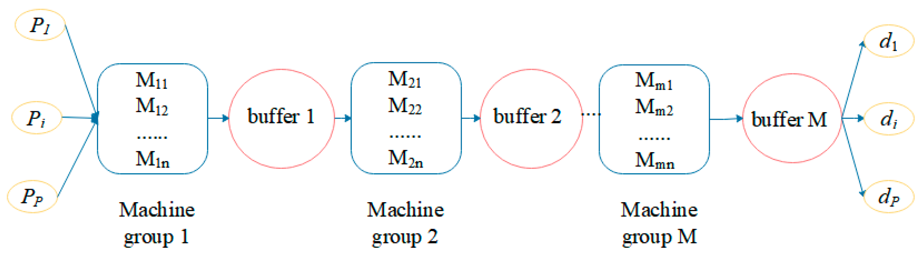
The production model of the manufacturing system studied in this paper is shown in Figure 1. It contains M different machine groups and M buffers, and it produces P product types. The machine groups are connected on a serial production line. Each machine group contains N identical parallel machines and has a buffer downstream, which is used to store work-in-process (WIP) or finished products, and the buffers are shared between the product types. Each machine has a different production capacity for each product type, but the production capacity of the machine is shared by the product types—that is, if a machine is produced with the full production capacity of a product type for the product type, then other product types cannot be produced at the same time by the machine.

The discrete manufacturing system in this paper uses the Flow-Shop scheduling [22] mode for processing; that is, the machine groups on the production line execute the different processes to complete the production order of the products, the processing procedure of the product types is the same, and they are processed only once in each machine group on the production line. The Flow-Shop scheduling model is a simplified model of many actual pipeline production scheduling problems, and it is also a typical non-deterministic polynomial hard (NP-hard) problem. Although the process constraints of Flow-Shop are relatively simple compared with Job-Shop scheduling (the processing route of each product type is not the same, and each product can be processed at most once on each machine), it is still a very complicated and difficult combinatorial optimization problem. Due to its NP-hard characteristics and strong engineering background, it has always been a hot issue in the theoretical and engineering fields. Therefore, the research on the Flow-Shop scheduling model has important theoretical significance and engineering value.

The production process of the system is as follows. All buffers are empty in the initial state; when the raw materials or semi-finished products of the products enter a machine group, one or more free and available machines are selected from the machine group to process. When the processing procedure is completed, the WIP or finished products are sent to the downstream buffer of the machine group for storage, waiting for the downstream machine group to take them away for processing in the next production stage. After all the processing procedures are completed, the finished products are sent to the last buffer for storage; when the demand order arrives, the finished products will be taken away from the last buffer corresponding to the demand.

Here are some assumptions for the manufacturing system:

(1)

It is assumed that the machines in the first machine group will not be hungry due to a lack of raw materials; that is, as long as the machines can process normally, raw materials are unlimitedly supplied.

(2)

It is a highly automated manufacturing system; therefore, the reassignment of production capacity costs little time, that is, the warm-up and cool-down time for each machine can be omitted.

(3)

The buffer capacity between machine groups is finite [23,24], that is, the machine will stop working because of blockage.

(4)

The machines are unreliable, that is, the machines may fail, and the failure only occurs when the machine is working, the idle machine will not fail;

We list the parameters and variables in the manufacturing system in

Table 1. The system parameters in the manufacturing system. WIP: work-in-process.

Parameters	Meanings	Type
M	the amount of the machine groups and the buffers	integer
N	the amount of the machines in each machine group	integer
P	the amount of product types	integer
T	the total discrete simulation time	integer
$s_k^{+}$	the inventory cost factor of WIP or finished product of product k in each buffer per unit of time	integer
$s_k^{-}$	the penalty factor for under-production of the finished product k in the end buffer per unit of time	integer
${\lambda }_{ik}$	the cost for supplementing the unit production capacity of machine group i for product k	integer
${\mu }_{ik}$	the initial production capacity of the machine in machine group i for product k (when other product types are not produced by the machine)	integer
$b_i$	the capacity of buffer i	integer
p	the failure rate of the machines, which obeys exponential distribution	real number
r	the repair rate of the machines, which obeys exponential distribution	real number
t_f	the average available time of the machines, which obeys uniform distribution	integer
t_r	the average unavailable time of the machines, which obeys uniform distribution	integer

,

Table 2. The system variables in the manufacturing system.

Variables	Meanings	Type
$y_{ik}(t)$	the inventory level of WIP or finished products of product k in buffer i at time t	real number
$y_{ik}^{+}(t)$	the amount of product k in the buffer i at time t	real number
$y_{Mk}^{-}(t)$	the amount of under-production of product k at time t	real number
$d_k(t)$	the demand rate of product k at time t	real number
${\varphi }_{ij}(t)$	the working status of the j-th machine in machine group i at time t, it will be 0 when the machine fails, and it will be 1 when the machine has been repaired	integer
${\phi }_i(t)$	the available status of supplementary production capacity in machine group i, it will be 0 when the production capacity is unavailable, and it will be 1 when the production capacity is available	integer

and

Table 3. The decision variables in the manufacturing system.

Variables	Meanings	Type
$u_{ik}(t)$	the real productivity of machine group i for product k at time t	real number
${\delta }_{ijk}(t)$	the actual productivity of the j-th machine in machine group i for product k at time t	real number
$Z_{ik}$	the hedging point of product k in buffer i	real number
$t_1$	the start time of supplementing production capacities in the machine groups	integer
$t_2$	the end time of supplementing production capacities in the machine groups	integer
$\Delta {\mu }_{ik}$	the supplementary production capacity of machine group i for product k during production	real number
$t_u$	the proportion of the time of supplementary production capacities $\Delta {\mu }_{ik}$ in the total discrete simulation time T, where $t_u=(t_2-t_1)/T$	real number

according to their types; the system parameters are shown in Table 1, they are constant and will not change in the production process.

The system variables are shown in Table 2, they change over time and are decided by the system parameters or the production process.

The decision variables are shown in Table 3; they need to be obtained through the PSO algorithm and the integrated control policy proposed in this paper.

The objective function, dynamic equations, and constraints of the multiple machines and multiple product types manufacturing system are given below.

2.1. Objective Function

The objective function is the total production cost, which consists of two parts: the first part is the inventory-related cost, and the second part is the cost of supplementary production capacities. The objective function is

$$\mathrm{Min}\frac{1}{T}\left[{\displaystyle \sum _{t=1}^T{\displaystyle \sum _{i=1}^M{\displaystyle \sum _{k=1}^{P}r(y_{ik}(t))+{\displaystyle \sum _{i=1}^M{\displaystyle \sum _{k=1}^{P}s(\Delta {\mu }_{ik})}}}}}\right].$$

(1)

The first part of the objective function is the sum of the storage costs and the costs of penalties for under-production of the products per unit time, it can be expanded into Equation (2).

$$\frac{1}{T}{\displaystyle \sum _{t=1}^T{\displaystyle \sum _{i=1}^M{\displaystyle \sum _{k=1}^{P}r(y_{ik}(t))=}}}\frac{1}{T}\left[{\displaystyle \sum _{t=1}^T{\displaystyle \sum _{i=1}^M{\displaystyle \sum _{k=1}^P{y}_{ik}^{+}(t)\cdot s_k^{+}+{\displaystyle \sum _{t=1}^T{\displaystyle \sum _{k=1}^P{y}_{Mk}^{-}(t)\cdot s_k^{-}}}}}}\right]$$

(2)

In Equation (2), $y_{ik}(t)$ is a system variable that will change over time, and it is determined by the production process where $y_{ik}^{+}(t)=max(y_{ik}(t),0)$, $y_{Mk}^{-}(t)=max(-y_{Mk}(t),0)$.

The second part of the objective function is the production cost of the supplementary production capacities, which can be expanded into Equation (3).

$$\frac{1}{T}{\displaystyle \sum _{i=1}^M{\displaystyle \sum _{k=1}^{P}s(\Delta {\mu }_{ik})=\frac{1}{T}}}{\displaystyle \sum _{i=1}^M{\displaystyle \sum _{k=1}^P\Delta {\mu }_{ik}\cdot {\lambda }_{ik}\cdot t_u}}$$

(3)

It can be seen from Equation (3) that the objective function does not include the costs of the machines themselves (including the initial production capacities); when the demands cannot be met, we will supplement the production capacities for the machine groups in a production cycle, and the supplementary production capacities $\Delta {\mu }_{ik}$ (non-negative) and the supplementary percentage of time $t_u$ are considered in the objective function. Where ${\lambda }_{ik}$ is a constant that will be given in the production process, $t_u$ can be calculated by $t_1$ and $t_2$. $\Delta {\mu }_{ik}$, $t_1$, and $t_2$ are the decision variables that need to be optimized by the PSO algorithm.

2.2. Dynamic Equation

The discrete form of the dynamic equation of inventory is

$$y_{ik}(t+1)=\{\begin{array}{ll}{y}_{ik}(t)+u_{ik}(t)-u_{i+1,k}(t),& if 1\le i\le M-1;\\ y_{ik}(t)+u_{ik}(t)-d_k(t),& if i=M;& \end{array}, k=1,\dots ,P$$

(4)

where $d_k(t)$ will be given in the simulation, it changes over time, and the value at each time t is known, while $u_{ik}(t)$ will be obtained by the integrated control policy.

The dynamic equation starts with the processing of the first machine group, and all buffers are empty in the initial state. The WIP processed in machine group i at time t will be sent to buffer i at time t + 1 after processing it, and the corresponding number of WIP in buffer i (i = 1, …, M − 1) at time t will be sent to machine group i + 1 according to the productivity of machine group i + 1 at time t; the corresponding number of finished products in buffer M will be taken away according to the demands at time t. Every production stage needs one time step (but not one second). Therefore, through Equation (4), how the inventory for each product type in each buffer changes dynamically on the serial production line can be seen.

2.3. Restrictions

The productivity of the machines and inventory status are constrained by many factors, and the factors will directly affect the production process. The constraints in the dynamic equations of the system are given below.

The first constraint on the productivity of the machine group is

$$0\le u_{ik}(t)\le y_{i-1,k}(t), i=2,\dots ,M,k=1,\dots ,P.$$

(5)

That is, the first machine group processes raw materials with unlimited supply, while the other machine groups process WIP processed by the previous machine group on the production line; therefore, the productivity of the machine group (except for the first one) must be no greater than the inventory level of the WIP in the upstream buffer.

The second constraint on the productivity of the machine group is

$$0\le u_{ik}(t)\le {\displaystyle \sum _{j=1}^N{\mu }_{ik}·{\varphi }_{ij}(t)}+\Delta {\mu }_{ik}·{\phi }_i(t), i=1,\dots ,M,k=1,\dots ,P$$

(6)

where ${\varphi }_{ij}(t)$ and ${\phi }_i(t)$ are determined by the failure mechanism of the machines or the supplementary production capacities in the machine groups. Due to the characteristics and the processing procedures of the machines in the different machine groups, the types of failure that may occur during production are different. Some types of machines can be guaranteed to be free from failure within a certain period of time. Some machines have lower costs but will fail at a certain frequency and need a certain amount of time to repair. The more common case is that the failure time and repair time obey an exponential distribution or uniform distribution [25,26,27]. The fault types are comprehensively considered in the manufacturing system.

Take the failure rate p and the repair rate r of the machines obeying exponential distribution, for example. The time between failures is an exponentially distributed random variable with average 1/p; then, ${\varphi }_{ij}(t)$ will be 1 during this period. The repair time is also exponentially distributed with average 1/r; then, ${\varphi }_{ij}(t)$ will be 0 during this period. The failure mechanism of the supplementary production capacity is the same as the machine group that uses it.

Equation (6) indicates that the productivities of the machine groups at any time must be no greater than the maximum production capacities of the machine groups (including supplementary production capacity possible), and the productivities are not negative.

The constraint on inventory level is

$$y_{ik}(t)\ge 0, i=1,\dots ,M-1,k=1,\dots ,P.$$

(7)

The inventory of the finished product can be negative, which indicates the number of under-production, and the inventory of all other WIP cannot be negative, the minimum is 0.

The buffer capacity is finite, and each buffer will store all the product types at the same time. Therefore, the inventory level of the product types will be limited by the buffer capacity and must satisfy:

$${\displaystyle \sum _{k=1}^P{y}_{ik}(t)}\le b_i, i=1,\dots ,M.$$

(8)

That is, the sum of the inventory level of all product types in each buffer at each moment must be no greater than the buffer capacity.

3. Integrated Control Policy

The integrated control policy can be divided into two parts, the first part is about the determination of the productivities of the machine groups based on the relationship between $Z_{ik}$ and $y_{ik}(t)$ on the production line, and the second part is about the allocation of the productivities of multiple parallel machines in the machine groups.

3.1. Production Control Policy for the Machine Groups

The priority of each product type is different according to the PHP control policy, and the production method is also different for the product type with different priority. The production control policy for the highest priority product type (k = 1) is expressed as follows:

$$u_{11}(t)=\{\begin{array}{l}\min \{{\displaystyle \sum _{j=1}^N{\mu }_{11}{\varphi }_{1j}(t)}+\Delta {\mu }_{11}{\phi }_1(t),\\ b_1-y_{11}(t)+u_{2,1}(t)\}, if y_{11}(t)<Z_{11}\\ \min \{{\displaystyle \sum _{j=1}^N{\mu }_{11}{\varphi }_{1j}(t)}+\Delta {\mu }_{11}{\phi }_1(t),u_{2,1}(t),\\ b_1-y_{11}(t)+u_{2,1}(t)\}, if y_{11}(t)=Z_{11}\\ 0,otherwise,\end{array}$$

(9)

$$\begin{gathered} u_{i1}(t)=\{\begin{array}{l}\min \{{\displaystyle \sum _{j=1}^N{\mu }_{i1}{\varphi }_{ij}(t)}+\Delta {\mu }_{i1}{\phi }_i(t),\\ b_i-y_{i1}(t)+u_{i+1,1}(t)\}, if y_{i1}(t)<Z_{i1}\\ \min \{{\displaystyle \sum _{j=1}^N{\mu }_{i1}{\varphi }_{ij}(t)}+\Delta {\mu }_{i1}{\phi }_i(t),u_{i+1,1}(t),\\ b_i-y_{i1}(t)+u_{i+1,1}(t)\}, if y_{i1}(t)=Z_{i1}\\ 0,otherwise,\end{array} \\ i=2,\dots ,M-1 \end{gathered}$$

(10)

$$u_{M1}(t)=\{\begin{array}{l}\min \{{\displaystyle \sum _{j=1}^N{\mu }_{M1}{\varphi }_{Mj}(t)}+\Delta {\mu }_{M1}{\phi }_M(t),\\ b_M-y_{M1}(t)+d_1(t)\}, if y_{M1}(t)<Z_{M1}\\ \min \{{\displaystyle \sum _{j=1}^N{\mu }_{M1}{\varphi }_{Mj}(t)}+\Delta {\mu }_{M1}{\phi }_M(t),d_1(t),\\ b_M-y_{M1}(t)+d_1(t)\}, if y_{M1}(t)=Z_{M1}\\ 0,otherwise,\end{array}$$

(11)

For the product type with the highest priority, the production control policy means that when the inventory level of the WIP or finished products in the buffer is less than its hedging point, the productivity of the machine group should be the minimum of the current maximum production capacity of the machine group (including the supplementary production capacity possible) and the remaining storage of the downstream buffer; when the inventory level of the WIP or finished products in the buffer is equal to its hedging point, the productivity of the machine group shall be the minimum of the productivity of the downstream machine group or demand rate, the remaining storage of downstream buffer, and the maximum production capacity of the machine group (including the supplementary production capacity possible) at the current moment. In other cases, the productivity of the machine group is 0.

The production control policy for the product type with the k-th (k = 2, …, P) highest priority is

$$\begin{gathered} u_{1k}(t)=\{\begin{array}{l}\min \{\left(1-{\displaystyle \sum _{m=1}^{k-1}\frac{u_{1m}(t)}{N·{\mu }_{1m}}}\right)·{\displaystyle \sum _{j=1}^N{\mu }_{1k}{\varphi }_{1j}(t)}+\Delta {\mu }_{1k}{\phi }_1(t),\\ b_1+{\displaystyle \sum _{m=1}^{k-1}(u_{2,m}(t)-y_{1m}(t)})\}, if y_{1k}(t)<Z_{1k}\\ \min \{\left(1-{\displaystyle \sum _{m=1}^{k-1}\frac{u_{1m}(t)}{N·{\mu }_{1m}}}\right)·{\displaystyle \sum _{j=1}^N{\mu }_{1k}{\varphi }_{1j}(t)}+\Delta {\mu }_{1k}{\phi }_1(t),u_{2,k}(t),\\ b_1+{\displaystyle \sum _{m=1}^{k-1}(u_{2,m}(t)-y_{1m}(t))}\}, if y_{1k}(t)=Z_{1k}\\ \\ 0,otherwise\end{array} \\ j=1,\dots ,N,k=2,\dots ,P \end{gathered}$$

(12)

$$\begin{gathered} u_{ik}(t)=\{\begin{array}{l}\min \{\left(1-{\displaystyle \sum _{m=1}^{k-1}\frac{u_{im}(t)}{N·{\mu }_{im}}}\right)·{\displaystyle \sum _{j=1}^N{\mu }_{ik}{\varphi }_{ij}(t)}+\Delta {\mu }_{ik}{\phi }_i(t),\\ b_i+{\displaystyle \sum _{m=1}^{k-1}(u_{i+1,m}(t)-y_{im}(t)})\}, if y_{ik}(t)<Z_{ik}\\ \min \{\left(1-{\displaystyle \sum _{m=1}^{k-1}\frac{u_{im}(t)}{N·{\mu }_{im}}}\right)·{\displaystyle \sum _{j=1}^N{\mu }_{ik}{\varphi }_{ij}(t)}+\Delta {\mu }_{ik}{\phi }_i(t),u_{i+1,k}(t),\\ b_i+{\displaystyle \sum _{m=1}^{k-1}(u_{i+1,m}(t)-y_{im}(t))}\}, if y_{ik}(t)=Z_{ik}\\ \\ 0,otherwise\end{array} \\ i=2,\dots ,M-1,j=1,\dots ,N,k=2,\dots ,P \end{gathered}$$

(13)

$$\begin{gathered} u_{Mk}(t)=\{\begin{array}{l}\min \{\left(1-{\displaystyle \sum _{m=1}^{k-1}\frac{u_{Mm}(t)}{N·{\mu }_{im}}}\right)·{\displaystyle \sum _{j=1}^N{\mu }_{Mk}{\varphi }_{Mj}(t)}+\Delta {\mu }_{Mk}{\phi }_M(t),\\ b_M+{\displaystyle \sum _{m=1}^{k-1}(d_m(t)-y_{Mm}(t))}\}, if y_{Mk}(t)<Z_{Mk}\\ \min \{\left(1-{\displaystyle \sum _{m=1}^{k-1}\frac{u_{Mm}(t)}{N·{\mu }_{im}}}\right)·{\displaystyle \sum _{j=1}^N{\mu }_{Mk}{\varphi }_{Mj}(t)}+\Delta {\mu }_{Mk}{\phi }_M(t),d_k(t),\\ b_M+{\displaystyle \sum _{m=1}^{k-1}(d_m(t)-y_{Mm}(t)})\}, if y_{Mk}(t)=Z_{Mk} \\ \\ 0,otherwise\end{array} \\ j=1,\dots ,N,k=2,\dots ,P \end{gathered}$$

(14)

For the products with the k-th highest priority, the production control policy means that when the inventory level of the WIP or finished products in the buffer is less than its hedging point, after the production capacity assigned to the product types with higher priorities, the remaining production capacity of the machine group is all assigned to it, and the actual productivity should be the minimum available production capacity of the machine group (including the supplementary production capacity possible) and the remaining storage of downstream buffer. When the inventory level of the WIP or finished products in the buffer is equal to its hedging point, the actual productivity of the machine group should be taken as the minimum of the productivity of the downstream machine group or demand rate, the remaining storage of downstream buffer, and the remaining production capacity of the machine group (including the supplementary production capacity possible). In other cases, the productivity of the machine group is 0.

3.2. The Allocation of the Productivities

According to the control policy in Equations (9)–(14), the productivities of the machine groups for the product types at time t is obtained. Since each machine group contains N identical parallel machines, the productivities of the machines in the machine groups at time t are determined by Equations (15)–(17).

We number the machines without failure in machine group i at time t from 1, and the first distribution method can be expressed by

$$\begin{gathered} {\delta }_{ijk}(t)=\{\begin{array}{ll}{u}_{ik}(t),& if u_{ik}(t)\le {\mu }_{ik}\&{\varphi }_{i1}(t)=1\\ 0,& otherwise\end{array} \\ i=1,\dots ,M,j=1,\dots ,N,k=1,\dots ,P. \end{gathered}$$

(15)

For machine group i that produces product k at time t, when the productivity of the machine group is less than the production capacity of each machine in the machine group, one machine without failure numbered 1 will be chosen to produce, and the productivity of the machine will be $u_{ik}(t)$, while other machines in the machine group will not produce for product k at time t.

To illustrate the second distribution method, we define the operational symbol “//” as exact division (keep the integer part of the division), and the operational symbol “%” as remainder after division. Then, make $\theta =u_{ik}(t)//{\mu }_{ik}$, which represents the amount of the machines with full production capacity in machine group i for product k at time t, and $\sigma =u_{ik}(t)\%{\mu }_{ik}$, which represents after using the full production capacity of $\theta$ machines, the surplus productivity required to be output in machine group i. The second distribution method for machine group i that produces product k at time t can be expressed by

$$\begin{gathered} {\delta }_{ijk}(t)=\{\begin{array}{ll}{\mu }_{ik},& if{\mu }_{ik}<u_{ik}(t)\le N·{\mu }_{ik}\\ & \&j=1,\dots ,\theta \&{\varphi }_{ij}(t)=1\\ \sigma ,& if {\mu }_{ik}<u_{ik}(t)\le N·{\mu }_{ik}\\ & \& j=\theta +1\& {\varphi }_{ij}(t)=1\\ 0,& otherwise\end{array} \\ i=1,\dots ,M,j=1,\dots ,N,k=1,\dots ,P. \end{gathered}$$

(16)

When the productivity of machine group i for product k at time t is more than the production capacity of each machine in machine group i, but less than the total production capacity of the machines in machine group i, the productivity of the machines in machine group i numbered 1 to $\theta$ without failure will be its maximum production capacity, and the productivity of the machine numbered $\theta +1$ will be $\sigma$; the other machines in the machine group will not produce for product k at time t.

The third distribution method can be expressed by

$$\begin{gathered} {\delta }_{ijk}(t)=\{\begin{array}{ll}{\mu }_{ik},& if N·{\mu }_{ik}<u_{ik}(t)\le N·{\mu }_{ik}+\Delta {\mu }_{ik}\\ & \&{\varphi }_{ij}(t)=1\\ 0,& otherwise\end{array} \\ i=1,\dots ,M,j=1,\dots ,N,k=1,\dots ,P. \end{gathered}$$

(17)

Equation (17) shows that when the productivity of machine group i for product k at time t is more than the total production capacity of the machines in machine group i, the productivity of all machines without failure in machine group i will be at their maximum production capacity, and the insufficient productivity is provided by the supplementary production capacity $\Delta {\mu }_{ik}$; the supplementary productivity by $\Delta {\mu }_{ik}$ will be $\min (\Delta {\mu }_{ik}·{\phi }_i(t),u_{ik}(t)-{\displaystyle \sum _{j=1}^N{\delta }_{ijk}(t)·{\varphi }_{ij}(t)})$ at time t.

3.3. The Decision Variables

In order to prevent the situation in which the production capacities of the machines cannot meet the constantly changing demands, considering the problems caused by the frequent supplement of the production capacities, such as credit and the movement and maintenance of the equipment, the production capacities are supplemented only once in one production cycle. According to the initial production capacities of the machines and the demands, the supplementary production capacities for the product types in the machines groups and the supplementary start and end time need to be optimized.

The production process can be divided into three stages and separated by the start time $t_1$ and end time $t_2$ of the supplementing production capacities in the machine groups. The decision variables are composed of the supplementary production capacities for the product types $\Delta {\mu }_{ik}$(i = 1, …, M, k = 1, …, P), the hedging points of the product types in the buffers at three stage $Z_{ik}$(i = 1, …, M, k = 1, …, P), and the start time $t_1$ and end time $t_2$ of supplementing production capacities.

The decision variables in the integrated control policy need to be optimized in order to minimize the objective function, and they are considered to be optimized by an intelligent optimization algorithm, such as genetic algorithm, ant colony algorithm, or PSO algorithm. These algorithms have different characteristics and application directions. The genetic algorithm mainly simulates the crossover, reproduction, and gene mutation phenomena in the genetic process and natural selection. The parameters of the combination, crossover, and mutation in the algorithm are mostly based on experience, and there are lots of parameters to be adjusted. It is mainly used to solve continuous function problems and combinatorial optimization problems. Ant colony algorithm is inspired by the behavior of observing how ants find their paths in the process of searching for food, it is a probability algorithm used to find the optimal path in the graph, and it is mainly used to solve graph coloring problems and vehicle routing problems.

The PSO algorithm is a search algorithm that has loose requirements for the function shape and has memory. Its iteration is updated on the basis of the optimal solution that has been found. It has a fast convergence speed and does not have lots of parameters that need to be adjusted. At present, the PSO algorithm has been widely used in the discrete optimal control problem of single-objective function and neural network training. In view of the multi-constraint, multi-variable, and single-objective optimization characteristics of the manufacturing system studied in this article, through the adjustment of the inertia weight parameters in the PSO algorithm, we first use the global PSO algorithm to search for the approximate range of the optimal solution quickly. Then, we use the local PSO algorithm to avoid falling into the local optimal solution. It is easier to obtain the optimal solution with PSO than with the genetic algorithm or ant colony algorithm. In summary, this paper uses the PSO algorithm to obtain the decision variables, combined with the integrated control policy given by Equations (9)–(17) to optimize the objective function, and the simulation process is implemented by Matlab.

4. Numerical Experiments

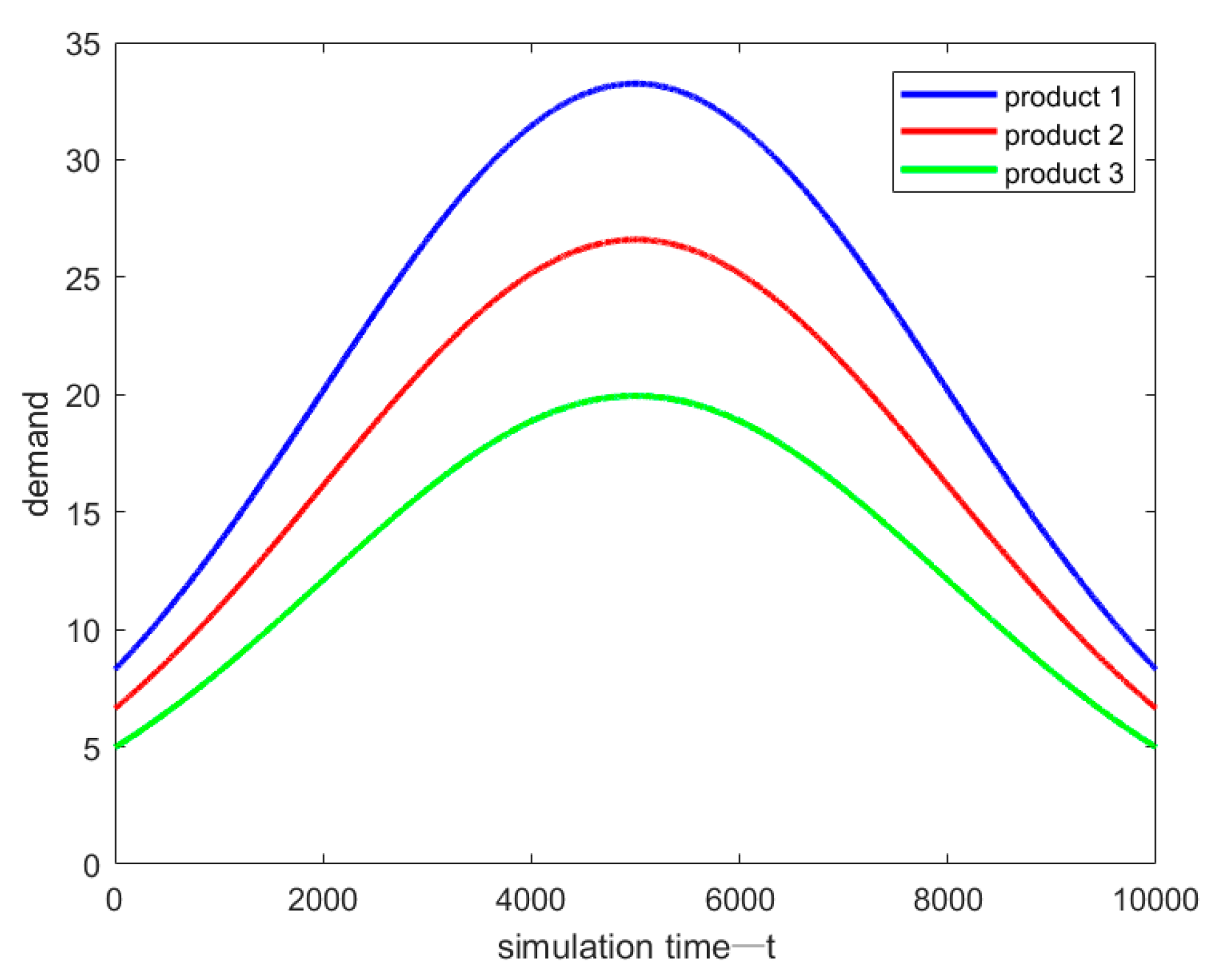
According to the PHP control policy, the priorities of the product types need to be sorted; it is comprehensively considered by their demands, storage costs, and penalty costs for under-production per unit time and the delivery times. Suppose that the storage costs and penalty costs of the product types are the same, and the delivery times of the product types are also the same. In order to obtain a more universal control policy, we assume that the demands are normally distributed in the simulation, and the curve of the demands of the product types over time is shown in Figure 2. According to the demands and assumption of the product types, product 1 can be designated as the highest priority product, followed by product 2 and product 3.

4.1. Simulation Experiments

Before conducting the simulation experiments, it is necessary to explain the various parameter settings of the manufacturing system. The objective function does not include the costs of the initial production capacities of the machines, but the initial production capacities of the machines will affect the objective function. As the initial production capacities of the machines increase, the probability of under-production and the objective function will decrease, but the initial production capacities of the machines cannot be too large, as they are limited by the practical manufacturing system. Therefore, the initial production capacities of the machines in the machine groups for the product types per unit time are taken as μ_i1 = 40, μ_i2 = 30, and μ_i3 = 20 (i = 1, …, M).

Assume that the amount of the machine groups in the manufacturing system M is 3, the amount of the machines in the machine groups N is 2, and the amount of product types P is 3. One simulation cycle T has 10,000 time units; the cost of storage of product k per unit time $s_k^{+}$ is 1, the penalty cost for an under-production of product k per unit time $s_k^{-}$ is 10 (k = 1, …, P); and the costs of supplementing the unit production capacity for the product types in the machine groups are taken as ${\lambda }_{1k}$ = 50,000, ${\lambda }_{2k}$ = 40,000, and ${\lambda }_{3k}$ = 30,000 (k = 1, …, P).

Most of the machines in the manufacturing system are unreliable. Within a simulation cycle, it is assumed that the machines in the first machine group will not fail, and the stability of the machines in the production process can be guaranteed by inspection during the gap between production cycles. The failure rate p and the repair rate r of the machines in the second machine group obey exponential distribution; then, 1/p and 1/r are the average time to failure and the average time to repair of the machines in the second machine group. The available time of the machines in the third machine group is uniformly distributed on the interval from t_f − 0.1t_f to t_f + 0.1t_f, and the unavailable time of the machines in the third machine group is uniformly distributed on the interval from t_r − 0.1t_r to t_r + 0.1t_r, then t_f and t_r are the average available time and the average unavailable time of the machines in the third machine group. For the machines in the second machine group, the failure rate p = 0.001 and the repair rate r = 0.1; for the machines in the third machine group, the average available time t_f = 2000, and the average unavailable time t_r = 20.

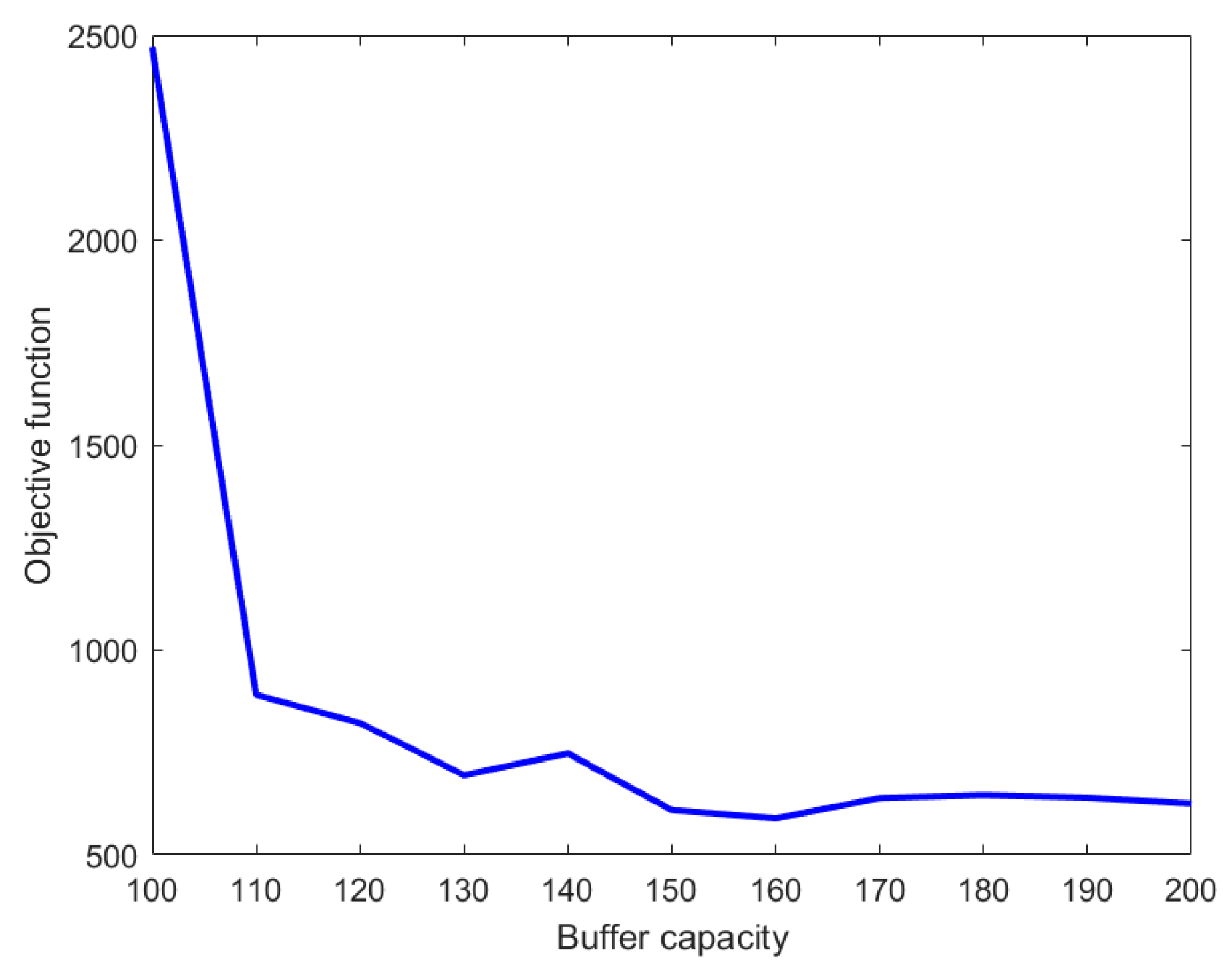
In order to clarify the impact of the buffer capacity on the objective function, under the assumption that the capacity of each buffer is identical and the system parameters given above, the simulation experiment on different buffer capacities is performed, and the experimental result is shown in Figure 3.

According to Figure 3, the objective function is decreasing with the increase of the buffer capacity. It becomes stable when the buffer capacity continues to increase, and there is almost no effect on reducing the objective function when the buffer capacity is bigger than 150. In order to minimize the impact of the buffer capacity on the objective function, the buffer capacities are taken as 150.

The simulation experiments are performed based on the integrated control policy and the system parameters given above, and the decision variables are optimized by the PSO algorithm to minimize the objective function. Since the production cost to be optimized in this article includes two parts, inventory cost and the cost of additional production capacity, in the process of group optimization by PSO algorithm, a cost objective is selected to calculate the particle fitness according to the principle of minimizing cost. Each generation of operations uses a strategy similar to dictionary sorting to optimize a goal. Through multiple experiments, the particle range and parameter settings that can minimize the total cost are determined. The values of the decision variables and each cost in the objective function are presented in

Table 4. The hedging points of the product types in the buffers at stage 1.

${\mathit{Z}}_{\mathit{i}\mathit{k}}$ at Stage 1	Product 1	Product 2	Product 3
Buffer 1	22.18	38.00	35.62
Buffer 2	20.54	27.85	28.11
Buffer 3	32.08	29.90	27.43

,

Table 5. The hedging points of the product types in the buffers at stage 2.

${\mathit{Z}}_{\mathit{i}\mathit{k}}$ at Stage 2	Product 1	Product 2	Product 3
Buffer 1	49.95	30.08	34.00
Buffer 2	37.44	43.01	46.37
Buffer 3	22.78	37.68	36.47

,

Table 6. The hedging points of the product types in the buffers at stage 3.

${\mathit{Z}}_{\mathit{i}\mathit{k}}$ at Stage 3	Product 1	Product 2	Product 3
Buffer 1	17.45	28.99	25.68
Buffer 2	33.20	34.07	11.64
Buffer 3	35.51	41.37	21.99

,

Table 7. The supplementary production capacities in the machine groups for the product types.

$\mathsf{\Delta }{\mathit{\mu }}_{\mathit{i}\mathit{k}}$	Product 1	Product 2	Product 3
Machine group 1	25.94	16.98	11.30
Machine group 2	13.11	16.34	22.38
Machine group 3	10.89	20.64	28.32

and

Table 8. The supplementary time of the production capacities and the costs.

Start Time t1	End Time t2	The Inventory Cost	The Cost of the Supplementary Production Capacities	The Total Production Cost
3329	6475	403.17	207.00	610.17

.

The experiment result shows that when $t<3329$, the hedging points for the product types in the buffers are shown in Table 4. When 6475 > t ≥ 3329, the production capacities of the machine groups are supplemented once for the product types to reduce the cost of under-production, the supplementary production capacities are presented as $\Delta {\mu }_{ik}$ (i = 1, … 3, k = 1, … 3) in Table 7, and the hedging points for the product types in the buffers are shown in Table 5. When t ≥ 6475, the production capacities of the machine groups return to the initial status, and the hedging points for the product types in the buffers are shown in Table 6. The production cost including the inventory cost and the supplementary production capacities cost are optimized and shown in Table 8.

4.2. Comparison with the PHP Control Policy

In order to illustrate the effectiveness of the integrated control policy proposed in this paper, based on the different initial production capacities of the machines, the control effect of the integrated control policy is compared with the PHP control policy adopted in [10] on the production line of different lengths. We compared the production cost under the two control policies when the length of the production line (the amount of the machine groups) is 3, 5, and 10 respectively, assuming that the system parameters of the even numbered machine group are the same as the second machine group, and the parameters of the odd numbered machine group (except the first machine group) are the same as the third machine group.

4.2.1. Experiment 1

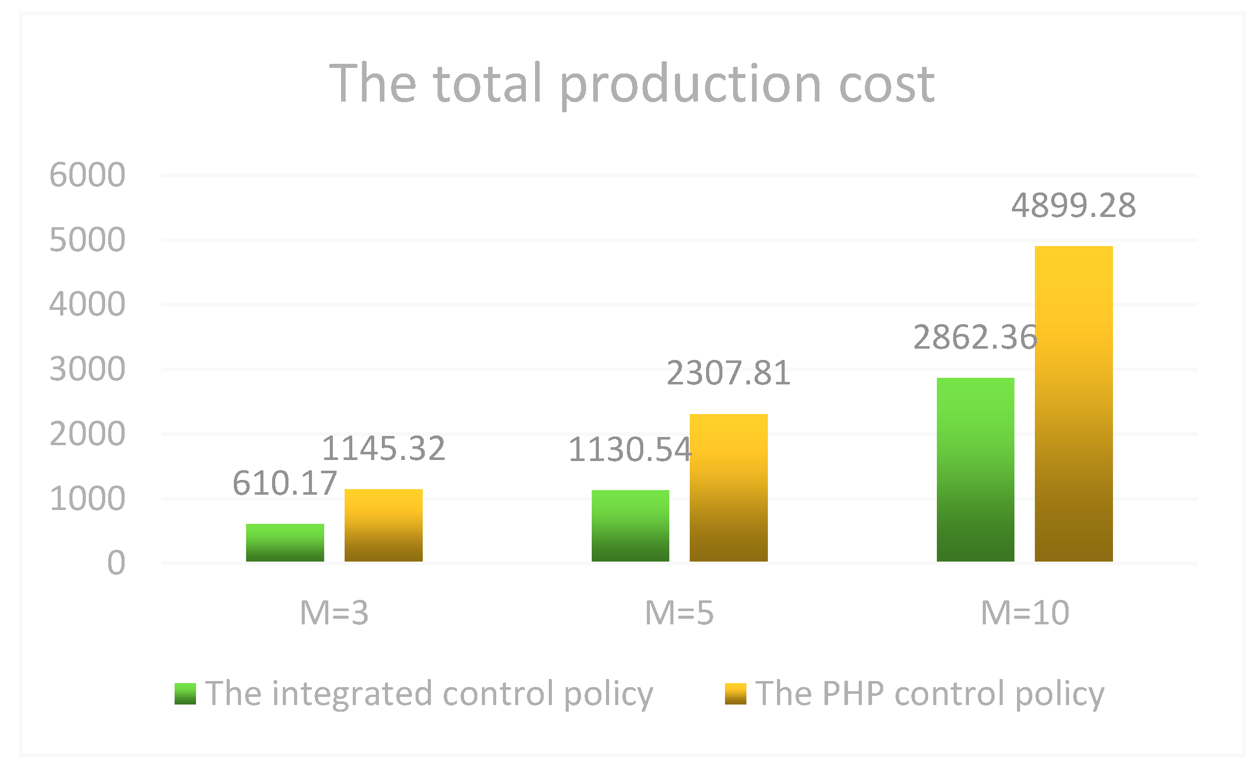
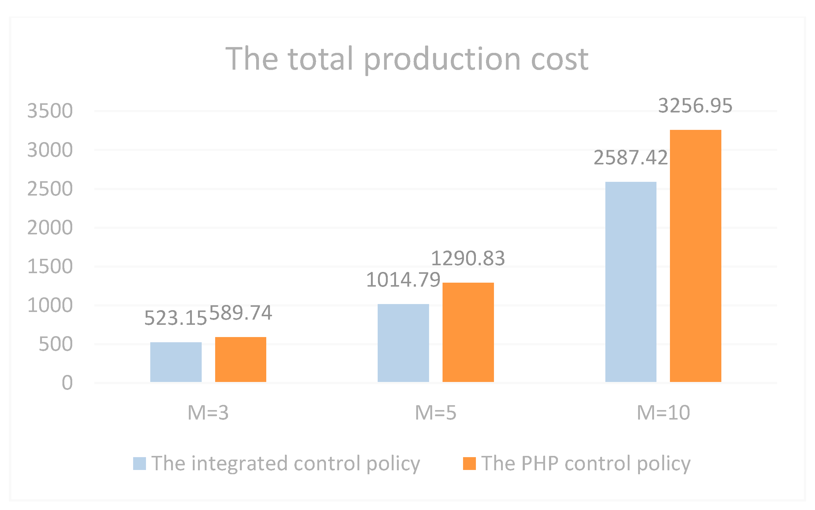
In Experiment 1, the initial production capacities of the machines on the production line are identical to 4.1; that is, ${\mu }_{i1}$ = 40, ${\mu }_{i2}$ = 30, ${\mu }_{i3}$ = 20 (i = 1, …, M). The experiment result is shown in Figure 4. From the data of the integrated control policy, when the length of the production line increases from 3 to 5, the total production cost is nearly doubled (increased from 610.17 to 1130.54), and when the length of the production line increases from 5 to 10, the total production cost has almost doubled (increased from 1130.54 to 2862.36), too. The experimental result shows that the integrated control policy has high stability in production cost control with the increase of the length of the production line. Meanwhile, under different lengths of the production line, the production costs of the integrated control policy are almost half of the PHP control policy adopted in [10]. It shows that for the multiple machines and multiple product types manufacturing system, when the initial production capacities of the machines cannot meet the demands in the production process, the integrated control policy shows obvious advantages compared with the PHP control policy adopted in [10] in production cost control.

4.2.2. Experiment 2

When the initial production capacities of the machines increase but still cannot meet the changing demands in the production process, in this case, we conducted another contrastive experiment in the production cost control of the two control policies. The initial production capacities increase from ${\mu }_{i1}$ = 40, ${\mu }_{i2}$ = 30, ${\mu }_{i3}$ = 20 (i = 1, …, M) to ${\mu }_{i1}$ = 45, ${\mu }_{i2}$ = 35, ${\mu }_{i3}$ = 25 (i = 1, …, M), and the other parameters are the same as those in Experiment 1; the experiment result is shown in Figure 5. When the initial production capacities of the machines increase, the probability of under-production and the cost of under-production will decrease in the production process. As a result, the total production cost under both policies has decreased compared with Experiment 1.

At the same time, as the initial production capacities of the machines increase, the production capacities that need to be supplemented in the production process to meet the demands will decrease; therefore, under the length of different production lines, the gap in production cost between the two control policies in Experiment 2 is reduced compared with Experiment 1. When the initial production capacities of the machines can fully meet the constantly changing demands during the production process, the control effects of the two control policies are almost the same (as the production capacities are no longer needed to be supplemented).

The experimental results in Experiment 1 and Experiment 2 show that for the multiple machines and multiple product types manufacturing system, when the initial production capacities of the machines can not meet the constantly changing demands, the control effect of the integrated control policy proposed in this paper is obviously better than the PHP control policy adopted in [10].

5. Conclusions and Further Research

In this paper, we analyze the problem of the production cost control for the multiple machines and multiple product types manufacturing system with uncertain fault. In order to reduce the occurrence of under-production and minimize the production cost under the constantly changing demands, an integrated control policy that combines the PHP control policy and the production capacity planning is proposed. The simulation experiments are conducted and show that when the initial production capacities of the machines can not fully meet the constantly changing demands during the production process, the integrated control policy proposed in the paper can reduce the production cost effectively compared with the PHP control policy adopted in [10]. For the production line with different lengths, the integrated control policy has shown high stability in production cost control. The integrated control policy proposed in this paper will provide a new research direction for the optimization in production cost control of the complex manufacturing systems.

The control policy proposed in this paper is studied on the mode of Flow-Shop system, in which the processing procedures and paths of each product are the same. In the practical manufacturing system, there are many cases where the processing paths of products are not identical and each product may pass through the same machine more than once. For this kind of manufacturing system, whether the optimization method proposed in this paper will be effective to control the production cost will be an interesting issue for further research.

References

- Kimemia, J.; Gershwin, S.B. An algorithm for the computer control of a flexible manufacturing system. IIE Trans. 1983, 15, 353–362. [Google Scholar] [CrossRef]
- Gershwin, S.B. Design and operation of manufacturing system control and system theoretical models and issues. In Proceedings of the 1997 American Control Conference, Albuquerque, NM, USA, 4–6 June 1997; pp. 1909–1913. [Google Scholar] [CrossRef]
- Perkins, J.R.; Srikant, R. Scheduling multiple part-types in an unreliable single-machine manufacturing system. IEEE Trans. Autom. Control 1997, 42, 364–377. [Google Scholar] [CrossRef]
- Kenne, J.P.; Gharbi, A. A simulation optimization based control policy for failure prone one-machine, two-product manufacturing systems. Comput. Ind. Eng. 2004, 46, 285–292. [Google Scholar] [CrossRef]
- Shu, C.; Perkins, J.R. Optimal PHP production of multiple part-types on a failure-prone machine with quadratic buffer costs. IEEE Trans. Autom. Control 2001, 46, 541–549. [Google Scholar] [CrossRef]
- Gharbi, A.; Kenne, J.P. Maintenance scheduling and production control of multiple-machine manufacturing systems. Comput. Ind. Eng. 2005, 48, 693–707. [Google Scholar] [CrossRef] [Green Version]
- Chan, F.T.S.; Wang, Z.; Zhang, J. Two-level hedging point control of a manufacturing system with multiple product-types and uncertain demands. Int. J. Prod. Res. 2008, 46, 3259–3295. [Google Scholar] [CrossRef]
- Senanayake, C.D.; Subramaniam, V. Analysis of a two-stage, flexible production system with unreliable machines, finite buffers and non-negligible setups. Flex. Serv. Manuf. J. 2013, 25, 414–442. [Google Scholar] [CrossRef]
- Mok, P. Evolutionary Optimisation of Production-Control Systems. Ph.D. Thesis, University of Hong Kong, Hong Kong, China, 2002. [Google Scholar] [CrossRef]
- Yan, H.S.; Jiang, T.H.; Meng, X.G. Hedging-point control policy for a failure-prone manufacturing system. Proc. Inst. Mech. Eng. B J. Eng. 2015, 231, 1479–1487. [Google Scholar] [CrossRef]
- Chen, W.; Wang, Z. Integrated capacity planning and production control of a parallel-machine manufacturing system. In Proceedings of the 2016 IEEE International Conference on Automation Science and Engineering (CASE), Fort Worth, TX, USA, 21–25 August 2016; pp. 401–406. [Google Scholar] [CrossRef]
- Kenne, J.P.; Boukas, E.K.; Gharbi, A. Control of production and corrective maintenance rates in a multiple-machine, multiple-product manufacturing system. Math. Comput. Model. 2003, 38, 351–365. [Google Scholar] [CrossRef]
- Filho, O.S.S. A constrained stochastic production planning problem with imperfect information of inventory. In Proceedings of the 16th IFAC World Congress, Prague, Czech Republic, 4–8 July 2005. [Google Scholar]
- Stephan, H.A.; Gschwind, T.; Minner, S. Manufacturing capacity planning and the value of multi-stage stochastic programming under Markovian demand. Flex. Serv. Manuf. J. 2011, 22, 143–162. [Google Scholar] [CrossRef]
- Mifdal, L.; Hajej, Z.; Dellagi, S. Joint optimization approach of maintenance and production planning for a multiple-product manufacturing system. Math. Probl. Eng. 2015, 2015, 1–17. [Google Scholar] [CrossRef]
- Ji, Q.; Wang, Y.; Hu, X. Optimal production planning for assembly systems with uncertain capacities and random demand. Eur. J. Oper. Res. 2016, 253, 383–391. [Google Scholar] [CrossRef]
- Liu, H.; Zhao, Q.; Huang, N. Production line capacity planning concerning uncertain demands for a class of manufacturing systems with multiple products. IEEE/CAA J. Autom. Sin. 2015, 2, 217–225. [Google Scholar] [CrossRef]
- Zhen, L. Optimization models for production and procurement decisions under uncertainty. Syst. Man Cybern. 2015, 46, 370–383. [Google Scholar] [CrossRef]
- Aghezzaf, E.; Sitompul, C.; Najid, N.M. Models for robust tactical planning in multi-stage production systems with uncertain demands. Comput. Oper. Res. 2010, 37, 880–889. [Google Scholar] [CrossRef]
- Ho, J.W.; Fang, C.C. Production capacity planning for multiple products under uncertain demand conditions. Int. J. Prod. Econ. 2013, 141, 593–604. [Google Scholar] [CrossRef]
- Huang, K.; Ahmed, S. A stochastic programming approach for planning horizons of infinite horizon capacity planning problems. Eur. J. Oper. Res. 2010, 200, 74–84. [Google Scholar] [CrossRef]
- Hermelin, D.; Shabtay, D.; Talmon, N. On the parameterized tractability of the just-in-time flow-shop scheduling problem. J. Sched. 2019, 22, 663–676. [Google Scholar] [CrossRef] [Green Version]
- Liu, C.; Zhu, Q.; Wei, F.; Rao, W.; Liu, J.; Hu, J.; Cai, W. A review on remanufacturing assembly management and technology. Int. J. Adv. Manuf. Tech. 2019, 105, 4797–4808. [Google Scholar] [CrossRef]
- Liu, C.; Cai, W.; Dinolov, O. Emergy based sustainability evaluation of remanufacturing machining systems. Energy 2018, 150, 670–680. [Google Scholar] [CrossRef]
- Vogl, G.W.; Weiss, B.A.; Helu, M. A review of diagnostic and prognostic capabilities and best practices for manufacturing. J. Intell. Manuf. 2019, 30, 79–95. [Google Scholar] [CrossRef] [PubMed]
- Kim, J.; Hwangbo, H. Real-Time Early Warning System for Sustainable and Intelligent Plastic Film Manufacturing. Sustainability 2019, 11, 1490. [Google Scholar] [CrossRef] [Green Version]
- Liu, C.; Zhu, Q.; Wei, F.; Rao, W.; Liu, J.; Hu, J.; Cai, W. An integrated optimization control method for remanufacturing assembly system. J. Clean. Prod. 2019, 248, 119261. [Google Scholar] [CrossRef]
Figure 1.
The production model of the multiple machines and multiple product types manufacturing system.
Figure 2.
The demands of three product types.
Figure 3.
Impact of the buffer capacity on the objective function.
Figure 4.
The total production cost under two control polities in Experiment 1.
Figure 5.
The total production cost under two control polities in Experiment 2.