Performance of Optimization Algorithms in the Model Fitting of the Multi-Scale Numerical Simulation of Ductile Iron Solidification

Abstract

The use of optimization algorithms to adjust the numerical models with experimental values has been applied in other fields, but the efforts done in metal casting sector are much more limited. The advances in this area may contribute to get metal casting adjusted models in less time improving the confidence in their predictions and contributing to reduce tests at laboratory scale. This work compares the performance of four algorithms (compass search, NEWUOA, genetic algorithm (GA) and particle swarm optimization (PSO)) in the adjustment of the metal casting simulation models. The case study used in the comparison is the multiscale simulation of the hypereutectic ductile iron (SGI) casting solidification. The model fitting criteria is the value of the tensile strength. Four different situations have been studied: model fitting based in 2, 3, 6 and 10 variables. Compass search and PSO have succeeded in reaching the error target in the four cases studied, while NEWUOA and GA have failed in some cases. In the case of the deterministic algorithms, compass search and NEWUOA, the use of a multiple random initial guess has been clearly beneficious.

1. Introduction

Today, numerical simulation of metal casting processes at macro scale is a well-known technology. Although new approaches based for example in dynamic mesh techniques are being currently investigated [1], the use of commercial programs based on the finite element method (FEM) or on the finite volume method (FVM) is quite widespread in the industry. However, the agreement between the obtained predictions and the actual results obtained at the foundry plant, is not always the desired one. This agreement is more difficult even in the case of multiscale simulation. For this reason, the model fitting is of high interest to improve the confidence in the predictions. Even more in the present context where, in one side the integrated computational materials engineering and in other side the hybrid prognostic models combining numerical simulation and data-driven models applied to the Industry 4.0 movement of the manufacturing industry, appear as two of the most promising and challenging research trends [2].

The obtaining of reliable predictions in metal casting processes is not a trivial task. The results do not only depend on numeric codes in which they are based. The use of the appropriate values of the thermophysical parameters along with the proper establishment of boundary conditions, is essential to avoid poor results or even erroneous ones. In fact, the ASM Committee [3] remarks that each manufacturing process has unique boundary conditions that can be even equipment specific, which must be identified and characterized for the specific application being simulated.

The characterization of the material properties for the whole range of temperatures involved in the metal casting processes is very difficult. Additionally, the determination of the values of some boundary conditions, as for example the heat transfer coefficients (HTC) between the alloy and the mold, is even more complex. The limitations of bibliographic data and the extreme difficulty of the direct determination of these values have inspired the application of inverse methods to avoid these difficulties.

The inverse methods can be considered a subset of the field of numerical optimization where the objective is to minimize one objective function, which represents the error between the simulation results and the experimental measurements. The challenge is that the corresponding objective function can be highly nonlinear or non-monotonic, may have a very complex form or its analytical expression may be unknown. Moreover, in the case of metal casting inverse problems, the effect of changes in boundary conditions are normally damped or lagged, i.e., the varying magnitude of the interior temperature profile lags behind the changes in boundary conditions and is generally of lesser magnitude. Therefore, such a problem would be a typically ill-posed and would normally be sensitive to measurement errors. Additionally, the uniqueness and stability of the solution are not generally guaranteed [4,5,6].

This type of optimization problems is usually solved using iterative strategies. The methodology consists basically in an iterative process where several parameters of the model are modified until the simulation predictions agree with the experimental measurements. Different strategies can be applied to advance in the iterative process depending on the selected optimization method.

In general, it is not possible to establish which optimization methods are the best between the high number of alternatives that exist. The performance of the optimization methods is completely related with the problem type to be tackled. Therefore, for each problem type, the most appropriate method should be searched.

The use of optimization algorithms to correlate the numerical models with experimental values has been applied in other fields different from the metal casting. The sector where possibly more efforts have been done in this sense, is the space industry. The correlation of the spacecraft thermal mathematical models with the results of the thermal tests is mandatory, which has encouraged the evaluation of different solutions. Some authors have explored the use of deterministic methods, as Klement, who used several quasi-newton type algorithms based on the Broyden methods [7,8] or Torralbo et al. who used a generalized iterative pseudo-inverse algorithm [9,10]. But most of them have studied and compared different stochastics methods. For example Dudon [11] use the Latin hypercube sampling (LHS), the self-adaptive evolution (SAE) and the branch and bound methods; Beck [12] use the adaptive particle swarm optimization (APSO); Van Zijl [13] use the Monte Carlo, the genetic algorithm (GA) and the APSO methods; Trinoga and Frey et al. [14,15] use the simulated annealing (SA), the threshold accepting (TA) and the GA; Anglada et al. work mainly with GA [16,17] but also made some comparisons with Klement algorithms [18] and with the deterministic algorithms TOLMIN, NEWUOA, BOBYQA and LINCOA [19]. In addition, works about the use of hybrid algorithms combining deterministic and stochastic methods can also be found, as the works of De Palo [20] where the downhill simplex is combined with the LHS or the work of Cheng et al. [21] where the Broyden–Fletcher–Goldfarb–Shanno (BFGS) is combined with the Monte Carlo method.

In contrast, the efforts done in the field of metal casting are much more limited. The number of bibliographic references devoted to the application of optimization algorithms to the adjustment of metal casting simulation models is quite reduced. Most of them [22,23,24,25] use the maximum A posteriori (MAP) algorithm, which is a variation of the least-square technique explained in reference [26]. Others perform the adjustment manually [27] or combining the manual adjustment with the MAP algorithm [28,29,30,31,32]. Moreover, some authors have tested different methods as Ilkhchy et al. [33] which use a nonlinear estimation technique similar to that stated by Beck in [34]; Dong et al. [35] that use a combined function specification and regularization method; Zhang et al. [36] with a neural network or Zhang et al. [37] that use a globally convergent method (GCM).

The authors of the present study believe that a deeper study in the performance of different optimization methods may contribute to give a step forward in the state of art of the model fitting applied to the metal casting. It would make possible to obtain adjusted models in less time and moreover will open the door to the future integration of automatic model fitting algorithms in prognostic models to be used in the framework of the industry 4.0.

The work presented henceforward compares the performance of several algorithms, deterministic and stochastic, in the adjustment of the multiscale simulation model of the solidification of a ductile iron casting, with the objective of contributing to the development of this research line in the search of a methodology solid enough to be used in the adjustment of metal casting simulation models.

2. Methodology

The methodology used for the adjustment of the simulation model is summarized in Figure 1.

The multiscale simulation model of the metal casting process was done with the commercial finite element software ProCAST 2018.0 (ESI Group, Paris, FRANCE), focused on metal casting simulation [38]. The fitness function represents the error between the simulation model predictions and the experimental results, that in this case are the alloy tensile strength. The parameters modification is guided by the optimization method used in each case, which was implemented by means of the PyGMO (Parallel Global Multiobjective Optimizer) library. PyGMO is a scientific library for massively parallel optimization developed in the context of the European Space Agency to evolve interplanetary spacecraft trajectories as well as designs for spacecraft parts and more [39].

2.1. Simulation Model

2.1.1. The Physics

Different approximations have been studied for the prediction of the tensile strength of cast alloys, as the use of machine learning algorithms [40] or analytical approximations as the Equation (1) stated by [41]. In this case, this last approximation, Equation (1), has been used by the simulation model to predict the tensile strength at room temperature $({\sigma }_{ULT})$, where $f_g$ is the graphite fraction, $n$ is the shape factor for graphite nodules which is related with their sphericity (maximum value, that is a perfect sphere, is unity), $f_{\alpha }$ is the ferrite fraction, $f_p$ the perlite fraction, and $\left(dT/dt\right){ }_{850}$ is the cooling rate at 850 °C. Therefore, the microstructure and the cooling rate must be previously calculated.

$${\sigma }_{ULT}=\left(1-f_g^n\right)\left(482.2f_{\alpha }+991.5f_p\right)+50\left[\left(dT/dt\right){}_{850}-0.5\right],$$

(1)

In cast irons the carbon and silicon contents are high, compared with steels, which origins a rich carbon content phase in their structure. When the alloy graphitization potential is high, which is determined by its composition and melt treatment, the iron solidifies according to the stable Fe-graphite system and the rich carbon phase is graphite, a hexagonal-close-pack form of carbon. In addition, the presence of magnesium makes the graphite structure be spheroidal instead of lamellar. One of the main melt treatments is the inoculation, which consists in the deliberate addition of elements that promote more active graphite nucleation sites (usually ferrosilicon enriched with Sr, Ba, Al, Zr, Ca and with very reduced and well calculated quantities of rare earths). The matrix structure is essentially determined by the composition and the cooling rate through the eutectoid temperature range. The eutectoid reaction leads to the decomposition of austenite into ferrite and graphite for the case of the stable eutectoid and to pearlite for the metastable eutectoid transformation. Slower cooling rates result in more stable eutectoid structure promoting a more ferritic matrix. If the complete transformation of austenite is not achieved when the metastable temperature is reached, pearlite forms and grows in competition with ferrite.

In the metal casting model used in this case, the influence of the chemical composition is managed by means of the thermodynamic database for multicomponent iron-based alloys developed by CompuTherm, PanFe 2017 (CompuTherm LLC, Middleton, WI, USA) [42]. This thermodynamic database is based on the calculation phase diagrams (CALPHAD) methodology, also called computer coupling of phase diagrams. CALPHAD is a materials genome method which plays a central and fundamental role in materials design, see reference [43] for more information. This method develops models to represent thermodynamic properties for various phases. The thermodynamic properties of each phase are described through the Gibbs free energy, based on the experimental and theoretical information available on phase equilibria and thermochemical properties in a system. Following this, it is possible to recalculate the phase diagram, as well as the thermodynamic properties, of all the phases and the system as a whole. It allows to reliably predict the set of stable phases and their thermodynamic properties in regions without experimental information and for metastable states during simulations of phase transformations together with the properties of multicomponent systems from those of binary and ternary subsystems. This is accomplished by considering the physical and chemical properties of the system in the thermodynamic model. In this case, the “lever” micro-segregation model, which assumes a complete mixing of the solute in the solid, was applied.

The influence of the melt treatment is managed by means of the nucleation parameters which must be specified/adjusted for each case, as they are not an intrinsic property of the material.

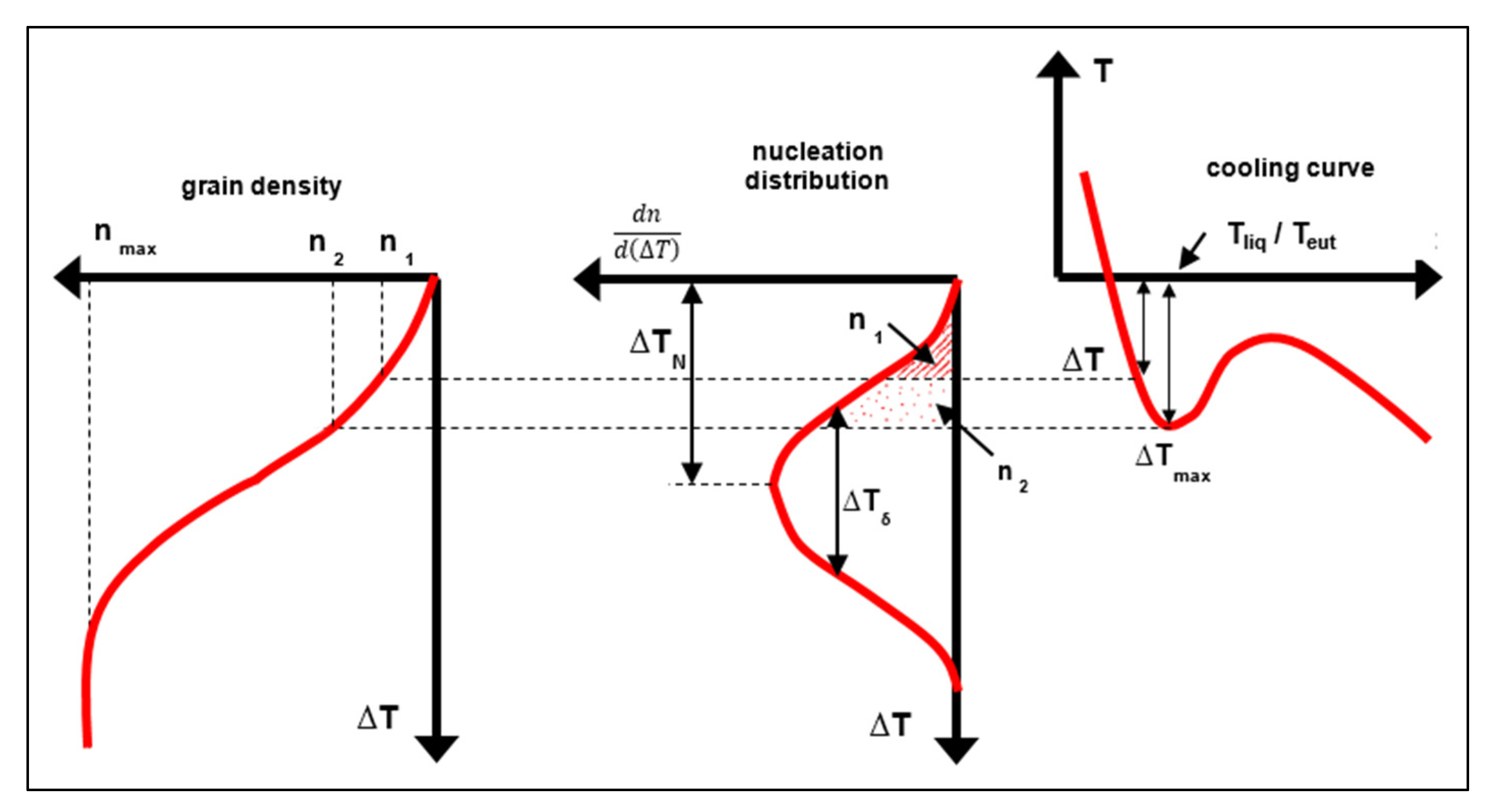
• The nucleation of the primary dendritic phase, austenite, is modeled following the gaussian distribution model proposed by [44]. This model defines the relationship between the number of nuclei and the undercooling ($∆T$) following Equation (2), where $n_{max}$ is the maximum grain nuclei density, $∆T_{\delta }$ the undercooling standard deviation and $∆T_n$ the average undercooling (see Figure 2):

  $$n\left(∆T\left(t\right)\right)=\frac{n_{max}}{\sqrt{2\pi }·∆T_{\delta }}{{\displaystyle \int }}_0^{∆T\left(t\right)}exp\left(-\frac{{\left(∆T\left(t\right)-∆T_n\right)}^2}{2∆T_{\delta }^2}\right)d\left(∆T\left(t\right)\right),$$

  (2)
• The nucleation of the graphite nodules is calculated as a power law of the undercooling following Equations (3) and (4) of the model proposed by [45], where $A_e$ and $n$ are the nucleation constants. This model assumes bulk heterogeneous nucleation at foreign sites which are already present within melt or intentionally added to the melt by inoculation:

  $$N_{eut}=A_e{\left(∆T\right)}^n,$$

  (3)

  $$\frac{d{N}_{eut}}{dt}=-n{A}_e{\left(∆T\right)}^{n-1}\frac{dT}{dt} ,$$

  (4)
• The graphite nodules growth is calculated with a quadratic power of the undercooling following Equation (5), where ${\mu }_e$ is the eutectic growth coefficient:

  $$\frac{d{R}_g}{dt}={\mu }_e{\left(∆T\right)}^2,$$

  (5)

Relating to the cooling rates, the governing equations of the physics involved in the mold filling, and in the alloy cooling and solidification, are the energy conservation, Equation (6), the mass conservation or continuity, Equation (7), and the Boussinesq form of the Navier–Stokes equation for incompressible Newtonian fluids, Equation (8), where $\rho$ is the density; $h$ is the specific enthalpy; $t$ is the time; $\upsilon$ is the velocity; $k$ is the thermal conductivity; ${\dot{R}}_q$ is the heat generation per unit mass; ${\rho }_0$ is density at reference temperature and pressure; $\widehat{p}$ is the modified pressure $\left(\widehat{p}=p+{\rho }_{0}gh\right)$; ${\mu }_l$ is the shear viscosity; $g$ is the gravity; ${\beta }_T$ is the volumetric thermal expansion coefficient; $T$ is the temperature and $T_0$ is the boundary temperature. More detailed information about them can be found at references [46,47].

$$\mathsf{\rho }\frac{\partial h}{\partial t}+\rho \upsilon ·\nabla h=\nabla ·\left(k\nabla T\right)+\rho {\dot{R}}_q,$$

(6)

$$\frac{\partial \rho }{\partial t}+\nabla ·\left(\rho \upsilon \right)=0$$

(7)

$${\rho }_0\left(\frac{\partial \upsilon }{\partial t}+\upsilon ·\nabla \upsilon \right)=-\nabla \widehat{p}+{\mu }_l{\nabla }^2\upsilon -{\rho }_{0}g{\beta }_T\left(T-T_0\right)$$

(8)

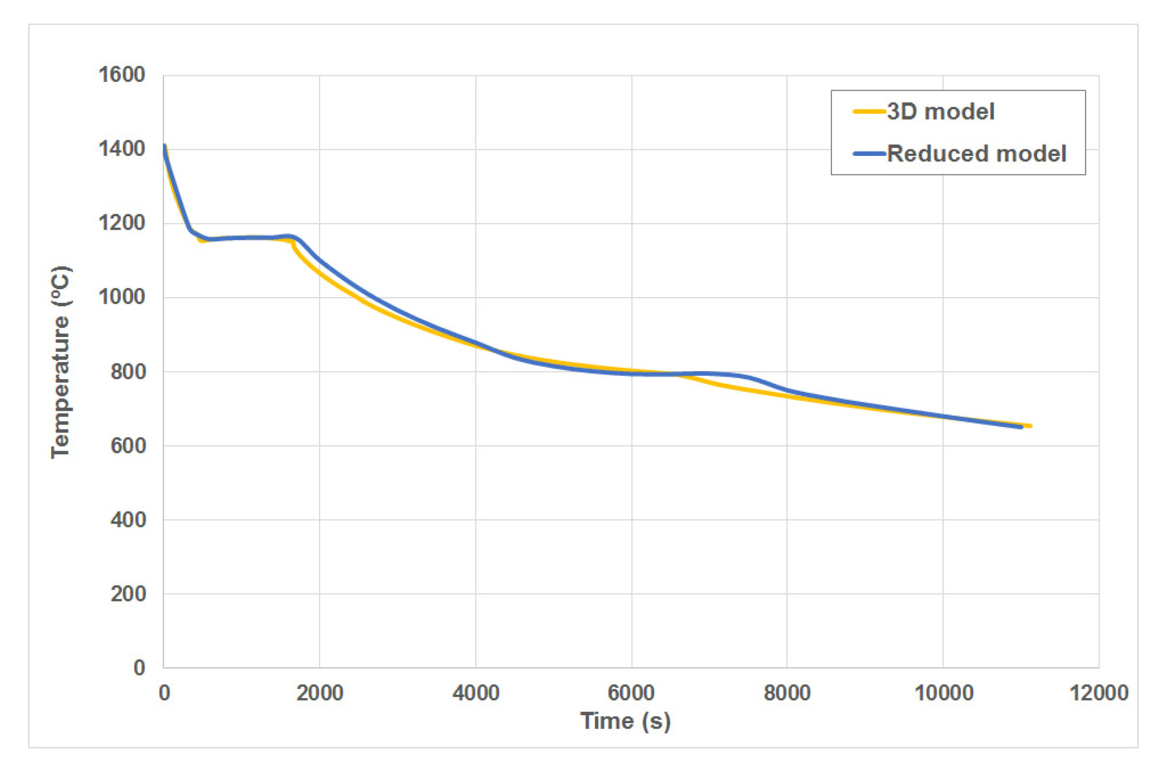
2.1.2. Model Reduction

A preliminary detailed 3D model has been developed. As can be observed in Figure 3a, it represents the complete geometry of the cast parts. The two similar, but different cast parts, the feeding systems formed by two risers, one for each cast part, the filling system and the mold. This 3D model is formed by 1,148,327 tetrahedral elements and 199,031 nodes. In this first attempt the complete simulation has been performed, that is, the part filling and the cooling and solidification process together with the microstructural calculations. The time step has taken values between 1 × 10⁻³ (during filling) and 50 s (during the last cooling) depending on the calculation evolution. The resolution of all the equations, shown in last section, for a transient analysis from pouring temperature (1410 °C) down to values below the eutectoid transformation temperature (738 °C), with the mentioned mesh and time steps, requires a high CPU time. In this case, the simulation has required about 5 h using a computer with 64 Gb of RAM using 8 cores Intel-Xeon CPU E5-2630 v3 @ 2.4 GHz (Dell Inc., Round Rock, TX, USA).

As it has been previously introduced, the model adjustment is an iterative procedure where the simulation model must be solved each time to get the predictions needed to calculate the fitness function. Therefore, it is highly advised to employ simulation models whose calculation times are as reduced as possible.

For this reason, due to the long calculation times of this model, a model reduction strategy was followed to reduce the high CPU time for the fitness function calculation. In first place the mold filling was suppressed from the calculation. As in this case the mold used was manufactured in resin bonded sand, the temperature drop during filling is not very pronounced. Therefore, the assumption of a mold completely filled of alloy at uniform temperature at the initial step of the simulation, is admissible. In second place the 3D geometry was replaced by a slice of the central area where the tensile test bar was extracted (see Figure 3b and Figure 5). This pseudo-2D geometry assumes that the heat flows mainly across the mold walls.

This model reduction presents some differences in the cooling rate (see Figure 4) which implies an error of 3.6% in the tensile strength prediction (433.64 MPa in the full 3D model and 418.14 MPa in the 2D model). However, the CPU time required to solve this 2D model is of only 29 s (620 times less). Therefore, regarding the CPU time saving, the error level is considered acceptable.

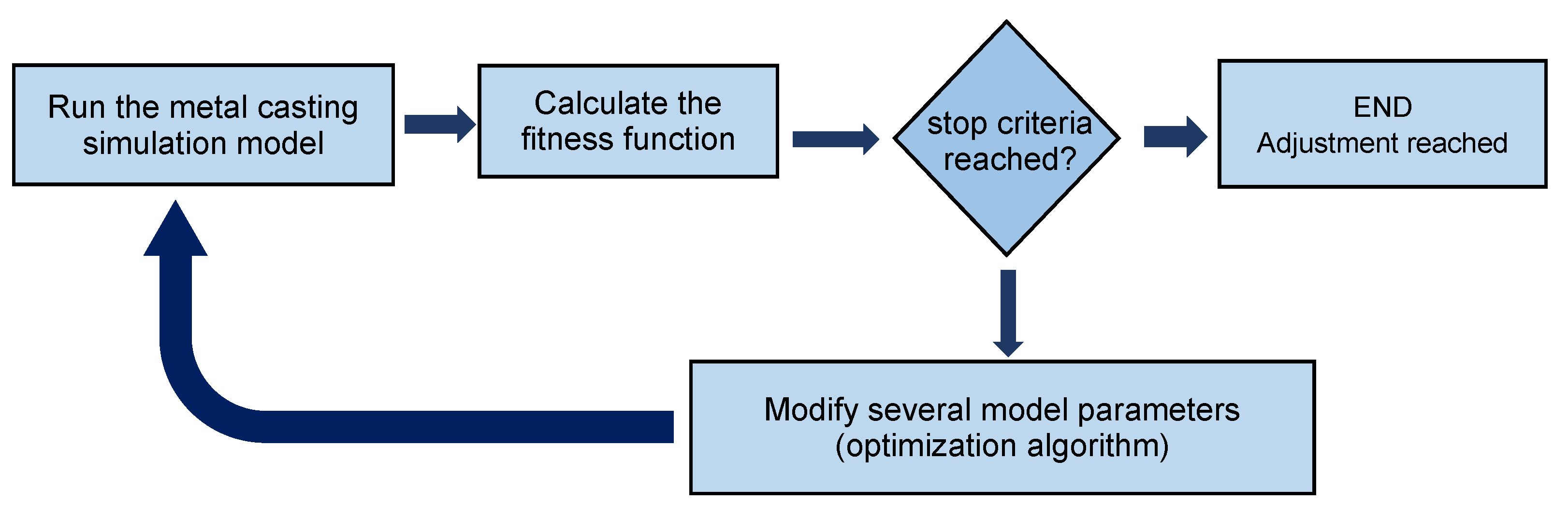
2.2. Fitness Function

The fitness function—also called cost function or objective function—is the mathematical representation of the aspect under evaluation which will be minimized. Therefore, it is the function that represents the difference between the hypothesis (model predictions) and the real results (experimental measurements), that is, the error. The expression used in this case, is the relative error between the predicted tensile strength (${\sigma }_{predicted}$) and the measured tensile strength (${\sigma }_{reference}$), following Equation (9). Note that absolute value of the difference is used.

$$fitness=\frac{\left|{\sigma }_{predicted}-{\sigma }_{reference}\right|}{{\sigma }_{reference}},$$

(9)

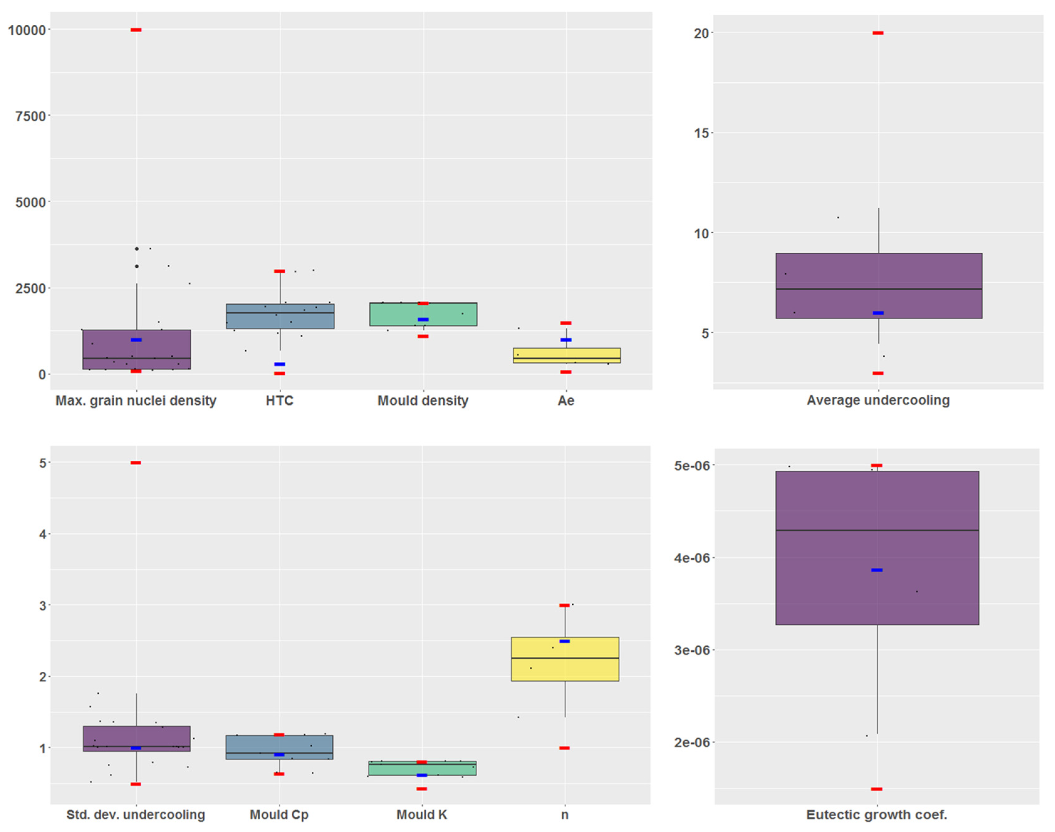
2.3. Variables Selection

The variables selection that is the parameters of the model that will be modified by the algorithm to adjust the model, was selected in a supervised mode based on the expert’s knowledge about the physics involved.

It is advised to select those variables which have more influence in the fitness function. Moreover, among them, those whose values are more uncertain. As it has been previously introduced, the tensile strength prediction is mainly related with the chemical composition of the alloy, the melt treatment and the cooling rate.

In this case the influence of the chemical composition is managed by the thermodynamic database, which calculates the material properties and the different phases that appears during the solidification. CALPHAD is a well-known methodology widely used in computational materials engineering, therefore, although new updated databases are continuously developed, we can assume its predictions as reliable.

The melt treatment can be modeled by means of the parameters that control the nucleation of the austenite: the maximum grain nuclei density $n_{max}$, the undercooling standard deviation $∆T_{\delta }$ and the average undercooling $∆T_n$; those that control the nucleation of the graphite nodules: $A_e$ and $n$; and, finally, the parameter that controls the graphite nodules growth, the eutectic growth coefficient ${\mu }_e$. All these parameters are very difficult to estimate, so they are good candidates to be included in the parameters group to be modified by the optimization method.

The cooling rate is mainly determined by the material properties of the alloy and the mold and for the heat transfer coefficient (HTC) between them. As said, the material properties of the alloy are calculated by the thermodynamic database, so they can be considered reliable. Resin bonded sand molds are manufactured mixing together clean and dry sand, with a binder and a catalyst in a continuous mixer. Different granulometries and types of sand can be used together with different binders and catalysts from several manufacturers, which can be also mixed in different proportions, so the resin bonded sand molds may present differences in their properties. Therefore, they can be also included in the parameters group to be modified by the optimization method. The heat transfer coefficient (HTC) between the alloy and the mold is difficult to estimate. When the metal enters in the mold, the macroscopic contact between the alloy and the mold is good because of the conformance of the molten metal. In this period the HTC presents high values, typically between 100 and 3000 W/m² K depending on different factors (surface roughness, pressure, wettability, etc.). Once a solidified layer with enough strength has grown, the contraction suffered by the alloy, together with the mold distortion caused by the mold heating, are likely to start a gap between them. In this phase, the HTC will mainly depend on the gas conductivity and the gap size, and its values may drop to values 10 times lower (10–100 W/m² K). In the ductile iron case, the expansion that takes place in the alloy during the graphite precipitation tends to reduce that gap but makes even more difficult the estimation of the HTC value. Therefore, the HTC is also a good candidate to be modified during the adjustment. However, in order to facilitate the implementation of the algorithm designed to perform the model fitting, a constant value was used for the HTC.

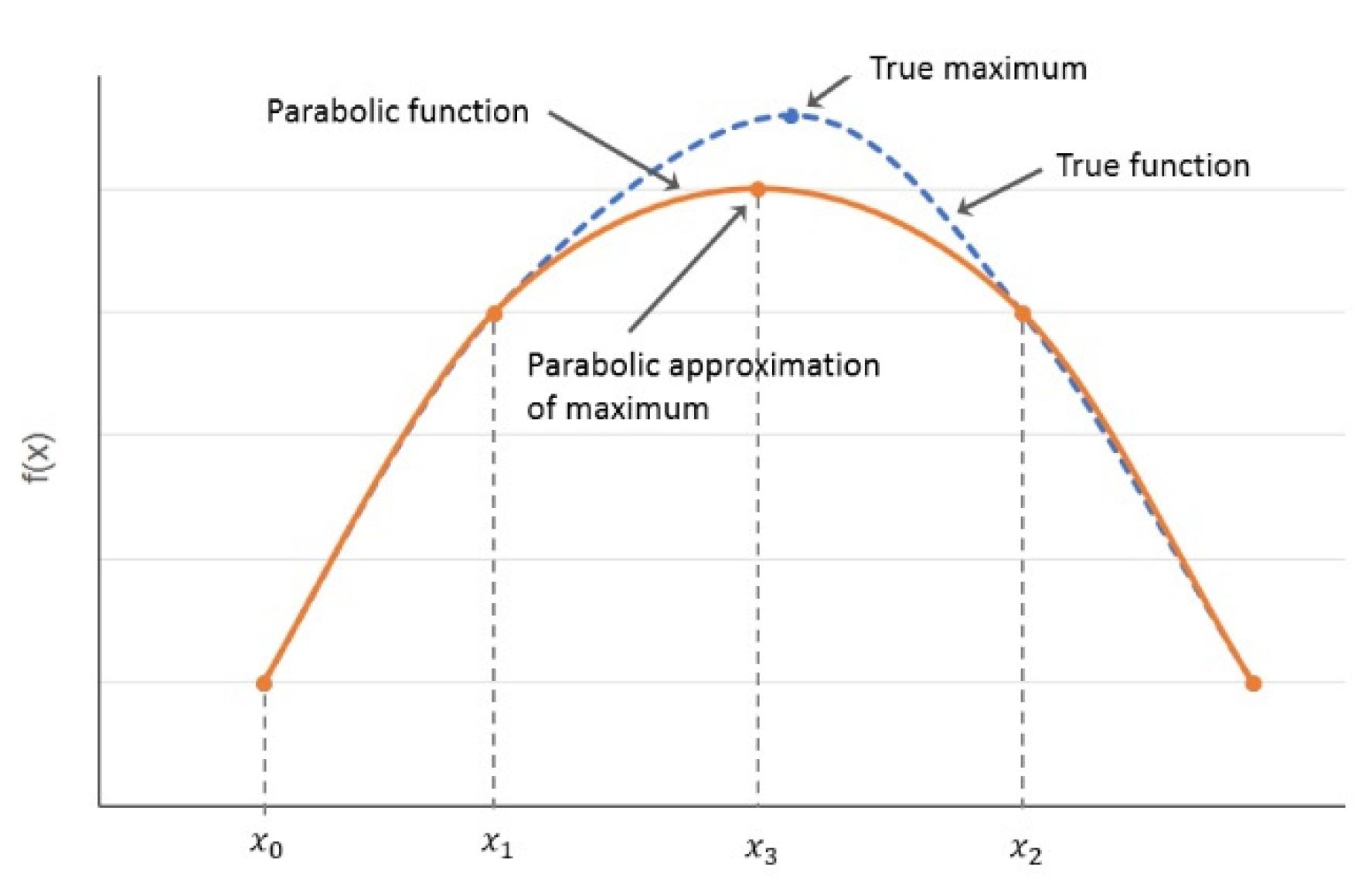
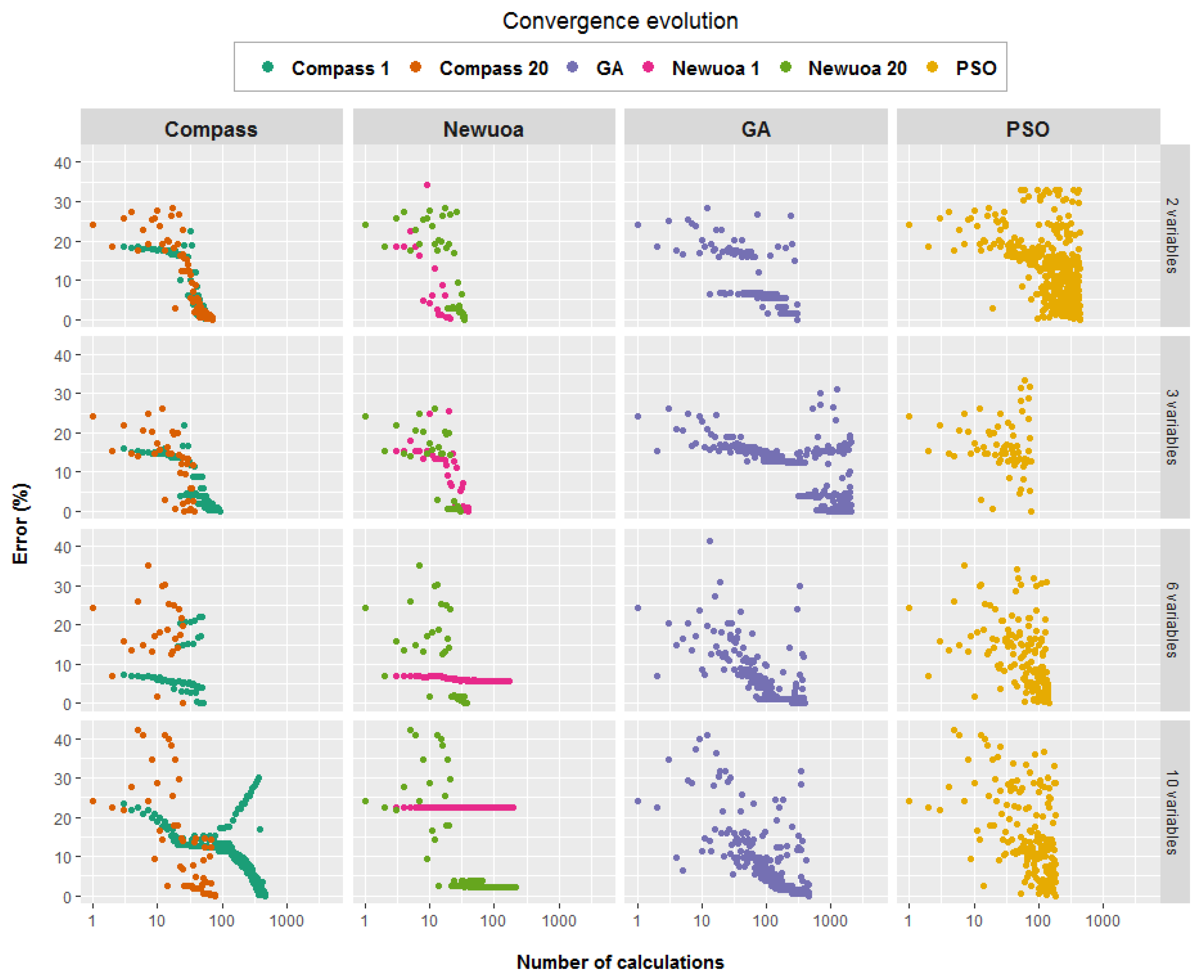
2.4. Optimization Methods

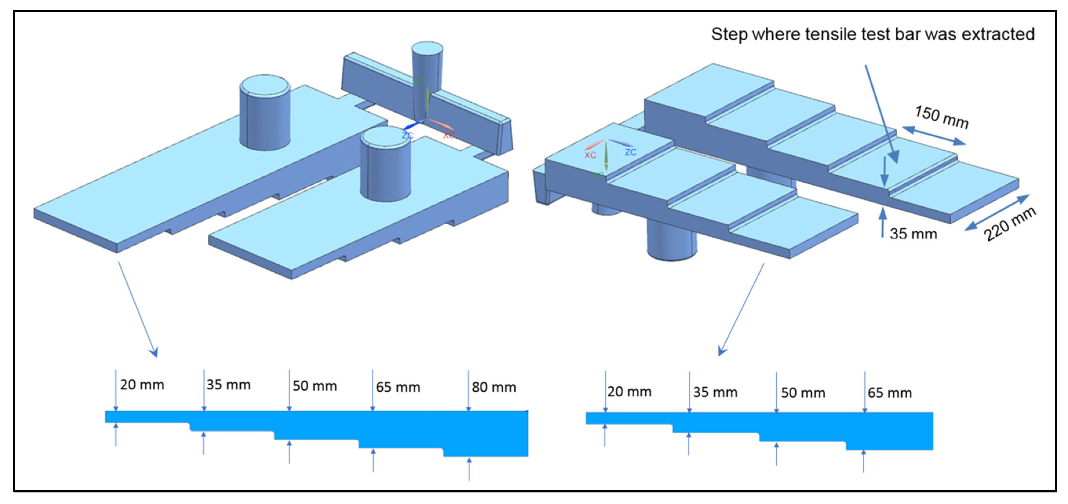
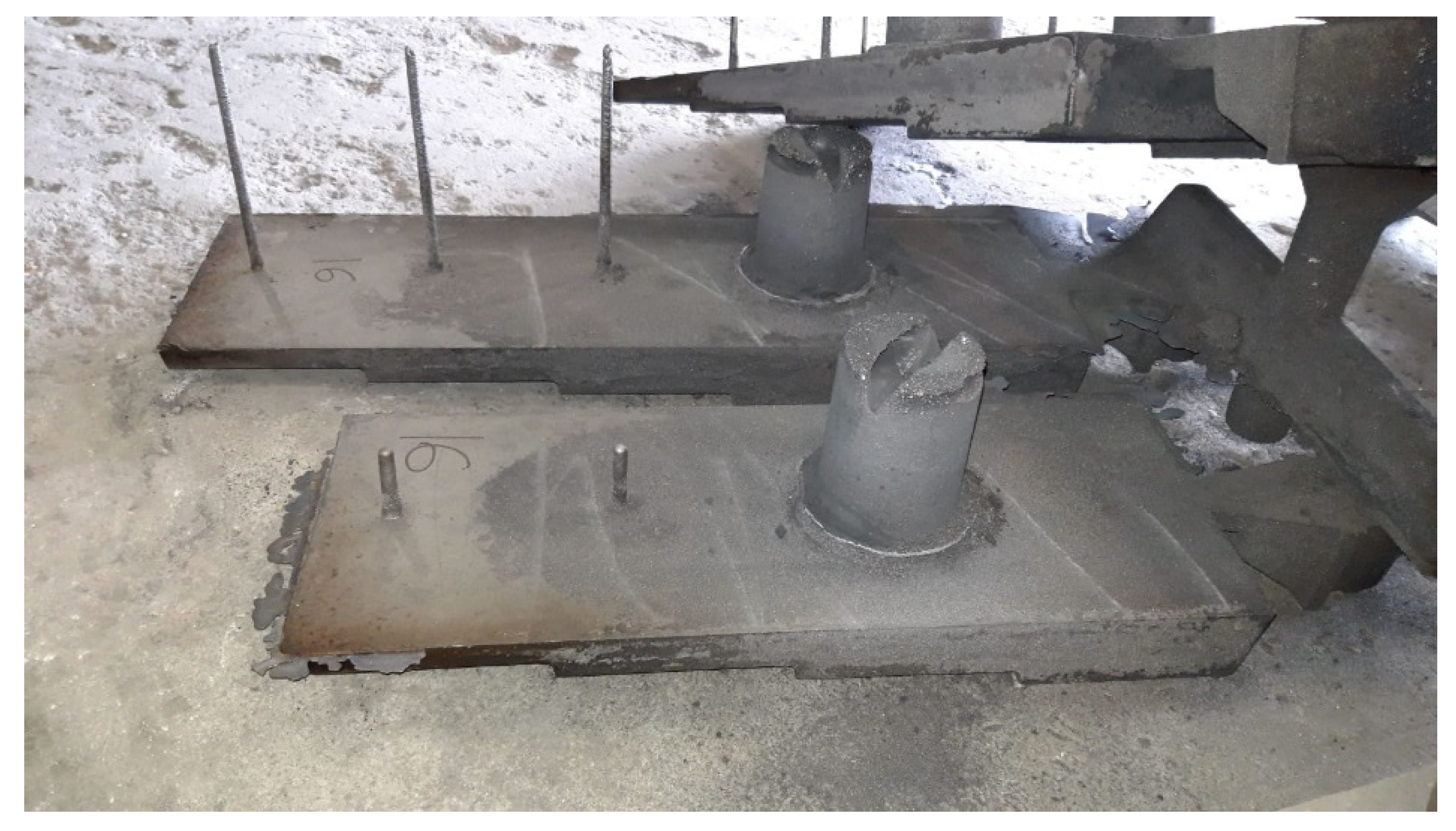
In the model fitting procedure followed, the parameters modification is guided by the optimization method. The performance of four different methods was compared. Two of them are deterministic methods, the compass search and the NEWUOA. The other two are heuristic methods, the particle swarm optimization (PSO) and the genetic algorithm (GA).

Compass search is a deterministic local optimization algorithm. It uses a simple and slow, but very sure procedure. The algorithm advances varying one of the parameters that form the solution vector at a time by steps of the same magnitude and when no such increase or decrease in any one parameter further improves the fit to the experimental data, they halve the step size and the process is repeated until the steps are deemed sufficiently small. For example, in a minimization problem with only two variables, the algorithm can be summarized as follows: Try steps to the East, West, North and South. If one of these steps yields a reduction in the function, the improved point becomes the new, iterate. If none of these steps yields improvement, try again with steps half as long. More details about this algorithm can be found in [48].

NEWUOA is also a deterministic local optimization algorithm. It seeks the least value of a function F without constraints and without derivatives. A quadratic approximation Q of the F function is used to obtain a fast convergence ratio, using a trust region strategy (see Figure 5). In this type of strategy, a model which represents a behavior similar to the objective function in a point $x_k$ is generated. The search of the optimum is restricted to the surroundings to that point, which is called trust region. As the optimization progress, successive approximations of Q are used. More details about this algorithm can be found in [49].

Particle swarm optimization (PSO) is a heuristic bioinspired algorithm for global optimization. A number of particles are placed in the search space of some problem or function and each evaluates the objective function at its current location. Each particle then determines its movement through the search space by combining some aspects of the history of its own current and best (best-fitness) locations with those of one or more members of the swarm, with some random perturbations. The next iteration takes place after all particles have been moved. Each individual in the particle swarm is composed of three D-dimensional vectors, where D is the dimensionality of the search space. The first vector is the current position $x_i$, which can be considered as a set of coordinates describing a point in space that is evaluated as a problem solution. Second vector is formed by the coordinates of previous best position $p_i$. The value of the best global position so far is stored in a variable for comparison on later iterations. The third vector is the velocity $v_i$, which can effectively be seen as a step size. In this way, new points are chosen by adding $v_i$ coordinates to $x_i$ and the algorithm operates by adjusting $v_i$. Each particle communicates with some other particles and is affected by the best point found by any member of its neighborhood. More details about this type of algorithm can be found in reference [50].

Genetic algorithms (GA) are heuristic search algorithms of general purpose inspired in the genetic processes that take place in biologic organisms and in the principles of the natural evolution of the populations. The basic idea consists in the generation of a random population of individuals or chromosomes and the advance to better individuals by means of the application of genetic operators, which are based in the genetic processes that takes place in the nature. Each of the individuals represents a possible solution to the problem, so the population represents the solutions search space. During the successive iterations, called generations, the individuals of the population are evaluated depending on their adaptation as solution. To do that, each one has associated a fitness value which measures how of good or bad is the possible solution that represents. The new population of individuals is created by selection mechanisms and by crossover and mutation operators. In this way, with the successive iterations or generations the algorithm converges to better solutions until reaching the optimum or the maximum number of iterations. More information about this type of algorithms can be found in reference [51].

3. Case Study

The case study is a part with a stepped geometry, cast in a sand mold bonded with resin where two similar parts are cast simultaneously. The reference value used for the model fitting is the tensile strength measured experimentally. Three tensile test bars were extracted from the central area of the 35-mm high step of the longer part, shown in Figure 6. The mean tensile strength obtained is equal to 552 MPa and the standard deviation equal to 4 MPa. The material is ductile iron, also called spheroidal gray iron (SGI), whose slightly hypereutectic composition is shown in

Table 1. Ductile iron chemical composition.

C (wt%)	Si (wt%)	Mn (wt%)	Cr (wt%)	Cu (wt%)	Mg (wt%)	CE	Tensile Strength (MPa)
3.53	2.65	0.27	0.037	0.37	0.04	4.404	552

, together with the tensile strength value measured experimentally. The mold was manufactured with silica sand mixed with a phenolic urethane resin (Pep-Set) and the corresponding catalyst. Figure 7 shows the manufactured cast part.

One important aspect in the performance of optimization algorithms is the dimensionality problem—that is, the number of variables that can be modified by the algorithm. Typically, classical optimization algorithms, as compass search or NEWUOA in this case, performs better in low dimensional problems, but when the number of variables increases it may require too long calculation times. Instead, the advantage of the heuristic algorithms, as PSO and GA in this case, takes place when the problem dimensionality is high. For this reason, the performance of the four optimization algorithms was evaluated for different numbers of variables included in the model fitting. The cases of 2, 3, 6 and 10 variables were studied. The corresponding variables considered in each case are detailed in

Table 2. Variables included in the model fitting cases.

Number of Variables	Variables
2	Parameters that control the nucleation of the graphite nodules: $A_e$ and $n$.
3	Parameters that control the nucleation of the graphite nodules: $A_e$ and $n$. HTC between the alloy and the mold
6	Parameters that control the nucleation of the graphite nodules: $A_e$ and $n$. HTC between the alloy and the mold. Density, thermal conductivity and specific heat of the mold
10	Parameters that control the nucleation of the graphite nodules: $A_e$ and $n$. HTC between the alloy and the mold. Density, thermal conductivity and specific heat of the mold. Parameters that control the nucleation of the austenite: Maximum grain nuclei density $n_{max}$, undercooling standard deviation $∆T_{\delta }$ and average undercooling $∆T_n.$Parameters that control the graphite nodules growth (eutectic growth coefficient ${\mu }_e$)

.

Table 3. Default values and ranges of the variables included in model fitting.

Parameter	Default Value	Minimum Value	Maximum Value
$A_e$	1.0 × 103	71.5	1500
$n$	2.5	1.0	3.0
HTCalloy-mold (W/m2 K)	300	30	3000
${\rho }_{mold}$ (kg/m3)	1590	1113	2067
$k_{mold}$ (W/mK)	0.621	0.435	0.808
${\left(C_p\right)}_{mold}$ (J/kgK)	914.0	640.0	1188.0
$n_{max}$	1.0 × 103	100	1.0 × 104
$∆T_{\delta }$ (°C)	1.0	0.5	5.0
$∆T_n$ (°C)	6.0	3.0	20.0
${\mu }_e$	3.87 × 10−6	1.5 × 10−6	5.0 × 10−6

summarize the default values used for these variables together with their ranges.

The optimization algorithms were used as they are implemented in the PyGMO library previously mentioned, using quite standard values for their internal parameters. Compass search was defined with a start range equal to 0.1, a stop range equal to 0.001 and a reduction coefficient equal to 0.5. In the case of NEWUOA, no additional parameters were setup. In order to compare both algorithms in similar conditions, the same seed were used in both cases.

Compass search and NEWUOA are local optimization algorithms, for this reason the selection of the initial guess may have influence in the final solution of the algorithm. For this reason, two different configurations were used for both. In the first configuration the algorithms are initialized with only one random guess. In the second one, they are initialized with 20 random guesses. In this last case, after the first iteration with those 20 individuals, the best of them is selected and the algorithms continue iterating from that point.

PSO and GA are stochastic population-based algorithms. In both cases a population size of 20 individuals were used. The canonical version of PSO based on the constriction coefficient velocity update formula was used. In addition, in this case quite standard values were used: constriction factor equal to 0.7298, social component equal to 2.05, a cognitive component equal to 2.05, maximum allowed particle velocities normalized respect to the bounds width equal to 0.5 and 4 individuals considered as neighbors. In the GA case, an exponential crossover operator with a probability equal to 0.90, a polynomial mutation operator with a probability equal to 0.02 and a tournament selection operator were used.

More details about the algorithm parameters can be found in [39].

4. Results and Discussion

The simulation model solved for the default parameters shown in Table 3, predicts a tensile strength value equal to 418.14 MPa, which corresponds to a relative error equal to 24% (see Equation (10)). The objective is to evaluate the ability of the algorithms to reduce that error to values below 0.1%, modifying the variables shown in Table 2.

$$\mathrm{Error}=\frac{\left|418.14-552\right|}{552}=0.2425,$$

(10)

Figure 8 collects the convergence evolution of each algorithm for the different cases studied. The behavior of the deterministic algorithms was uneven. The performance of the compass search was very good, reducing the error to values below the 0.1% in all cases with a reasonable number of calculations. The use of 20 initial random points has improved the algorithm performance reducing the number of calculations, especially in the 10 variables case where the difference is clear.

NEWUOA algorithm instead, failed in reaching the error target in several cases. Using an initialization based on only one point, the algorithm has failed in the 6 and 10 variables cases with error values equal to 22.62% and 5.77%, respectively. The use of 20 random initial points clearly has improved the behavior of the algorithm making possible to reach the target in the 6 variables case and to reduce the error value to 2.07% in the 10 variables case.

The heuristic algorithms, GA and PSO, have succeeded in reaching the error target in all the cases, with the exception of the GA in the 3 variables case, where the minimum error value was equal to 0.124%. The number of calculations needed to reach the target error was lower for PSO than for GA, except for the 2 variables case.

Therefore, the best options were the compass search algorithm with 20 random initial points, followed by the PSO algorithm.

A priori, it can be thought that as higher the number of variables, larger the search domain and higher the difficulty of the algorithm to reach the target. However, a higher number of variables may also imply a bigger number of solutions that fulfil the target value, making easy to find one of them. On the other side, a reduced number of variables may be too restrictive limiting the number of possible solutions and making difficult to reach the target. The results obtained are not clear in this sense. There is a tendency in the deterministic algorithms to find more difficulties in cases with higher number of variables in contrast with the heuristics, which have found more difficulties in cases with a lower number of variables. However, the obtained results are not conclusive in this sense.

Relating to the values assigned to the variables, as it was explained in the introduction, it does not exist a unique solution of the problem. Therefore, the model may be fitted assigning different combinations of the values assigned to the variables. The risk of this fact is that sometimes, the values assigned to the variables by the algorithm may cause a certain loss in the physical sense of the model although the results are accurate from the mathematical point of view. However, this is a common difficulty of this type of approximation that has not been solved by now.

Figure 9 shows the distribution of the values assigned to the different variables in boxplot form. Black points represent the values assigned for each variable jittered, the blue line corresponds to the value assigned for each variable in the initial model and red lines to the bounds fixed for each of them (In the case of NEWUOA no bounds are used). As can be observed the distribution is quite different depending on the adjusted variable.

Figure 10 collects the values assigned grouped by the number of variables included in the fitting and colored by the algorithm used in each case. Colored bars represent the values assigned to the variables by the different optimization algorithms, the dotted red lines represent the bounds fixed for the corresponding variable and the dotted blue line the value initially assigned.

As expected, the higher the number of variables included in the adjustment, the higher the variability in the values assigned. This can be observed in the cases of the maximum grain nuclei density, the undercooling standard deviation and the heat transfer coefficient. Otherwise, the variability of the values assigned to the variable seems also related with the algorithm used. For example, compass search presents a bigger tendency to adjust the variable to higher values. However, as the “true” value of each variable is actually unknown, it is difficult to evaluate if any of the algorithms has a better performance in assigning more reliable values to the variables.

5. Conclusions

Only compass search and PSO have succeeded in reaching the error target in the four cases studied (2, 3, 6 and 10 variables). The NEWUOA and GA algorithms have failed in some case.

In the case of the deterministic algorithms, compass search and NEWUOA, the use of a multiple random initial guess was clearly beneficious.

Compass search with an initial 20 random points has presented the best performance, reaching the error target in all cases with the lower number of calculations.

The known problem related with the absence of a unique solution was found, obtaining different combinations of the values assigned to the variables. However, as the ‘true’ value of each variable is actually unknown, it is difficult to evaluate if any of the algorithms has a better performance in assigning more reliable values to the variables.

Future works. The authors believe that the research line focused in the fitting of metal casting models by means of optimization algorithms is very interesting, as the advances in this area may contribute to reduce the time needed to adjust the metal casting models improving the confidence in their predictions and contributing to reduce tests at laboratory scale. In fact, some of the future works planned are:

▪

Model fitting based on several properties, for example ultimate and yield strengths. It would be a very interesting improvement in this type of technique, although it would imply to tackle a multi-objective optimization, much more challenging that the classical optimization presented in this work;

▪

Evaluate the results obtained in this study for a completely different type of material (for example some aluminum alloy or superalloy) and/or for a different manufacturing casting process (for example die casting or investment casting);

▪

Include the possibility of using temperature dependent variables in the model fitting.

References

1. Horr, A.M.; Kronsteiner, J. On numerical simulation of casting in new foundries: Dynamic process simulations. Metals 2020, 10, 886. [Google Scholar] [CrossRef]
2. Diez-Olivan, A.; Del Ser, J.; Galar, D.; Serra, B. Data fusion and machine learning for industrial prognosis: Trends and perspectives towards Industry 4.0. Inf. Fusion 2019, 50, 92–111. [Google Scholar] [CrossRef]
3. ASM. International Handbook Committee ASM Handbook, Metals Process Simulation, 1st ed.; Furrer, D.U., Semiatin, S.L., Eds.; ASM International: Novelty, OH, USA, 2010; Volume 22B, ISBN 978 1 61503 005 7. [Google Scholar]
4. Gadala, M.S.; Vakili, S. Assesment of Various Methods in Solving Inverse Heat Conduction Problems. In Heat Conduction—Basic Research; Vikhrenko, V., Ed.; InTech: Rijeka, Croatia, 2011; pp. 37–62. ISBN 978-953-307-404-7. [Google Scholar]
5. Beck, J.V.; Blackwell, B.; St. Clair, C.R. Inverse Heat Conduction: Ill-Posed Problems; John Wiley & Sons Inc: Hoboken, NJ, USA, 1985; ISBN 0-471-08319-4. [Google Scholar]
6. Özisik, M.N.; Orlande, H.R.B. Inverse Heat Transfer: Fundamentals and Applications; Taylor & Francis: New York, NY, USA, 2000; ISBN 1-56032-838-X. [Google Scholar]
7. Klement, J. On using quasi Newton algorithms of the Broyden class for model-to-test correlation. In Proceedings of the 28th European Space Thermal Analysis Workshop, Noordwijk, The Netherlands, 14–15 October 2014; ESA, Ed.; ESA Publications Division: Noordwijk, The Netherlands, 2014; pp. 213–228. [Google Scholar]
8. Klement, J. On Using Quasi-Newton Algorithms of the Broyden Class for Model-to-Test Correlation. J. Aerosp. Technol. Manag. 2014, 6, 407–414. [Google Scholar] [CrossRef] [Green Version]
9. Torralbo, I.; Perez-Grande, I.; Sanz-Andrés, A.; Piqueras, J. Correlation of Thermal Mathematical Models to test data using Jacobian matrix formulation. In Proceedings of the 48th International Conference on Environmental Systems ICES-2018, Alburquerque, NM, USA, 8–12 July 2018. [Google Scholar]
10. Torralbo, I.; Perez-Grande, I.; Sanz-Andres, A.; Piqueras, J. Correlation of spacecraft thermal mathematical models to reference data. Acta Astronaut. 2017. [Google Scholar] [CrossRef] [Green Version]
11. Dudon, J.P.; Pasquier, H.M. Evaluation of stochastic & statistics methods for spacecraft thermal analysis. In Proceedings of the 25th European Workshop on Thermal and ECLS Software, Noordwijk, The Netherlands, 8–9 November 2011; ESA, Ed.; ESA Publications Division: Noordwijk, The Netherlands, 2011; pp. 319–335. [Google Scholar]
12. Beck, T.; Bieler, A.; Thomas, N. Numerical thermal mathematical model correlation to thermal balance test using adaptive particle swarm optimization (APSO). Appl. Therm. Eng. 2012, 38, 168–174. [Google Scholar] [CrossRef]
13. Van Zijl, N.; Zandbergen, B.; Benthem, B. Correlating thermal balance test results with a thermal mathematical model using evolutionary algorithms. In Proceedings of the 27th European Space Thermal Analysis Workshop, Noordwijk, The Netherlands, 3–4 December 2013; ESA, Ed.; ESA Publications Division: Noordwijk, The Netherlands, 2013; pp. 89–108. [Google Scholar]
14. Trinoga, M. Development of an automated thermal model correlation tool. In Proceedings of the 28th European Space Thermal Analysis Workshop, Noordwijk, The Netherlands, 14–15 October 2014; ESA, Ed.; ESA Publications Division: Noordwijk, The Netherlands, 2014; pp. 201–212. [Google Scholar]
15. Frey, B.; Trinoga, M.; Hoppe, M.; Ebeling, W.D. Development of an Automated Thermal Model Correlation Method and Tool. In Proceedings of the 45th International Conference on Environmental Systems, ICES 2015, Washington, DC, USA, 12–16 July 2015; ICES STEERING COMMITTEE, Ed.; Texas Tech University: Lubbock, TX, USA, 2015; pp. 1–14. [Google Scholar]
16. Anglada, E.; Garmendia, I. Correlation of thermal mathematical models for thermal control of space vehicles by means of genetic algorithms. Acta Astronaut. 2015, 108, 1–17. [Google Scholar] [CrossRef]
17. Garmendia, I.; Anglada, E. Thermal mathematical model correlation through genetic algorithms of an experiment conducted on board the International Space Station. Acta Astronaut. 2016, 122, 63–75. [Google Scholar] [CrossRef]
18. Klement, J.; Anglada, E.; Garmendia, I. Advances in automatic thermal model to test correlation in space industry. In Proceedings of the 46th International Conference on Environmental Systems, ICES 2016, Vienna, Austria, 10–14 July 2016; ICES STEERING COMMITTEE, Ed.; Texas Tech University: Lubbock, TX, USA, 2016; pp. 1–11. [Google Scholar]
19. Anglada, E.; Martinez-Jimenez, L.; Garmendia, I. Performance of Gradient-Based Solutions versus Genetic Algorithms in the Correlation of Thermal Mathematical Models of Spacecrafts. Int. J. Aerosp. Eng. 2017, 2017, 1–12. [Google Scholar] [CrossRef]
20. De Palo, S.; Malosti, T.; Filiddani, G. Thermal Correlation of BepiColombo MOSIF 10 Solar Constants Simulation Test. In Proceedings of the 25th European Workshop on Thermal and ECLS Software, Noordwijk, The Netherlands, 8–9 November 2011; ESA, Ed.; ESA Publications Division: Noordwijk, The Netherlands, 2011; pp. 271–284. [Google Scholar]
21. Cheng, W.; Liu, N.; Li, Z.; Zhong, Q.; Wang, A.; Zhang, Z.; He, Z. Application study of a correction method for a spacecraft thermal model with a Monte-Carlo hybrid algorithm. Chin. Sci. Bull. 2011, 56, 1407–1412. [Google Scholar] [CrossRef] [Green Version]
22. Opstelten, I.J.; Rabenberg, J.M. Determination of the thermal boundary conditions during aluminium DC casting from experimental data using inverse modelling. In Essential Readings in Light Metals; Grandfield, J.F., Eskin, D.G., Eds.; Springer: Berlin/Heidelberg, Germany, 2016; p. 7. [Google Scholar]
23. Leder, M.O.; Gorina, A.V.; Kornilova, M.A.; Tarenkova, N.Y.; Kondrashov, E.N. Determination of the Thermophysical Properties of Titanium Alloys from Liquid Bath Profiles. Russ. Metall. 2015, 12, 964–969. [Google Scholar] [CrossRef]
24. Torroba, A.J.; Koeser, O.; Calba, L.; Maestro, L.; Carreño-Morelli, E.; Rahimian, M.; Milenkovic, S.; Sabirov, I.; LLorca, J. Investment casting of nozzle guide vanes from nickel-based superalloys: Part I—Thermal calibration and porosity prediction. Integr. Mater. Manuf. Innov. 2014, 3–25. [Google Scholar] [CrossRef] [Green Version]
25. Jin, H.; Li, J.; Pan, D. Application of inverse method to estimation of boundary conditions during investment casting simulation. Acta Metall. Sin. (Engl. Lett.) 2009, 22. [Google Scholar] [CrossRef] [Green Version]
26. Rappaz, M.; Bellet, M.; Deville, M. Inverse Methods. In Numerical Modeling in Materials Science and Engineering; Springer Series in Computational Mathematics; Springer: Berlin/Heidelberg, Germany, 2010; pp. 447–477. [Google Scholar]
27. Long, A.; Thornhill, D.; Armstrong, C.; Watson, D. Determination of the heat transfer coefficient at the metal-die interface for high pressure die cast AlSi9Cu3Fe. Appl. Therm. Eng. 2011, 31, 3996–4006. [Google Scholar] [CrossRef]
28. Anglada, E.; Meléndez, A.; Vicario, I.; Arratibel, E.; Aguillo, I. Adjustment of a High Pressure Die Casting Simulation Model against Experimental Data. Procedia Eng. 2015, 132, 966–973. [Google Scholar] [CrossRef] [Green Version]
29. Meléndez, A.; Anglada, E.; Maestro, L.; Dominguez, I. More robust processes and more added value for foundries based on inverse modelling and tailor-made software tools. In Proceedings of the 71st World Foundry Congress—Advanced Sustainable Foundry, Bilbao, Spain, 19–21 May 2014; Tabira Foundry Institute, WFO, IK4 Azterlan: Bilbao, Spain, 2014. [Google Scholar]
30. Meléndez, A.; Anglada, E.; Rodriguez, P.P.; Armenteros, A. Investment Casting Moulds Optimisation by means of Advanced Simulation and Instrumented Fibre-wrapped Moulds. In Proceedings of the European Investment Casters’ Federation (EICF). Technical Workshop for Foundry Engineers—Method Engineering & Process Modelling, Rotherham, UK, 12–13 May 2015. [Google Scholar]
31. Anglada, E.; Meléndez, A.; Maestro, L.; Dominguez, I. Adjustment of Numerical Simulation Model to the Investment Casting Process. Procedia Eng. 2013, 63, 75–83. [Google Scholar] [CrossRef] [Green Version]
32. Anglada, E.; Meléndez, A.; Maestro, L.; Dominguez, I. Finite Element Model Correlation of an Investment Casting Process. Mater. Sci. Forum. Adv. Mater. Process. Technol. MESIC V 2014, 797, 105–110. [Google Scholar] [CrossRef] [Green Version]
33. Ilkhchy, A.F.; Jabbari, M.; Davami, P. Effect of pressure on heat transfer coefficient at the metal/mold interface of A356 aluminum alloy. Int. Commun. Heat Mass Transf. 2012, 39, 705–712. [Google Scholar] [CrossRef] [Green Version]
34. Beck, J. V Nonlinear estimation applied to the nonlinear inverse heat conduction problem. Int. J. Heat Mass Transf. 1970, 13, 703–716. [Google Scholar] [CrossRef]
35. Dong, Y.; Bu, K.; Dou, Y.; Zhang, D. Determination of interfacial heat-transfer coefficient during investment-casting process of single-crystal blades. J. Mater. Process. Technol. 2011, 211, 2123–2131. [Google Scholar] [CrossRef]
36. Zhang, L.; Li, L.; Ju, H.; Zhu, B. Inverse identification of interfacial heat transfer coefficient between the casting and metal mold using neural network. Energy Convers. Manag. 2010, 51, 1898–1904. [Google Scholar] [CrossRef]
37. Zhang, W.; Xie, G.; Zhang, D. Application of an optimization method and experiment in inverse determination of interfacial heat transfer coefficients in the blade casting process. Exp. Therm. Fluid Sci. 2010, 34, 1068–1076. [Google Scholar] [CrossRef]
38. ProCAST. Version 2018.0. ESI Group: Paris, France. Available online: https://www.esi-group.com/products/casting (accessed on 1 July 2020).
39. Biscani, F.; Izzo, D. Esa/Pagmo2: Pygmo 2.15.0 (Version v2.15.0). Zenodo. Available online: https://ui.adsabs.harvard.edu/abs/2019zndo...2529931B/abstract (accessed on 2 April 2020).
40. Fragassa, C.; Babic, M.; Perez Bergman, C.; Minak, G. Predicting the Tensile Behaviour of Cast Alloys by a Pattern Recognition Analysis on Experimental Data. Metals 2019, 9, 557. [Google Scholar] [CrossRef] [Green Version]
41. Stefanescu, D.M.; Catalina, A.V.; Guo, X.; Chuzhoy, L.; Pershing, M.A.; Biltgen, G.L. Prediction of room temperature microestructure and mechanical properties in ductile iron castings. In Proceedings of the 4th Decennial International Conference on Solidification Processing, Sheffield, UK, 7–10 July 1997; p. 7. [Google Scholar]
42. PanFe. Version 2017. CompuTherm LLC: Middleton, WI, USA. Available online: https://computherm.com (accessed on 1 July 2020).
43. Chen, Q. CALPHAD and Beyond—The True Story of Materials Genome. In Proceedings of the International Forum on Advanced Materials, IFAM 2016, Nanjing, China, 24–26 September 2016; p. 22. [Google Scholar]
44. Rappaz, M.; Thevoz, P.H. Solute diffusion model for equiaxed dendritic growth: Analytical solution. Acta Metall. 1987, 35, 2929–2933. [Google Scholar] [CrossRef]
45. Oldfield, W. Freezing of Cast Irons. ASM Trans. 1966, 59, 945–959. [Google Scholar]
46. Dantzig, J.A.; Rappaz, M. Solidification; Dantzig, J.A., Rappaz, M., Eds.; CRC Press: Boca Raton, FL, USA, 2009; ISBN 978 0 8493 8238 3. [Google Scholar]
47. Lewis, R.W.; Ravindran, K. Finite element simulation of metal casting. Int. J. Numer. Methods Eng. 2000, 47, 29–59. [Google Scholar] [CrossRef]
48. Kolda, T.G.; Lewis, R.M.; Torczon, V. Optimization by Direct Search: New Perspectives on Some Classical and Modern Methods. SIAM Rev. 2003, 45, 385–482. [Google Scholar] [CrossRef]
49. Powell, M.J.D. The NEWUOA software for unconstrained optimization with derivatives. In Large-Scale Nonlinear Optimization; Di Pillo, G., Roma, M., Eds.; Springer: New York, NY, USA, 2006; pp. 255–297. ISBN 978-0387-30063-4. [Google Scholar]
50. Poli, R.; Kennedy, J.; Blackwell, T. Particle swarm optimization. Swarm Intell. 2007, 1, 33–57. [Google Scholar] [CrossRef]
51. Herrera, F.; Lozano, M.; Verdegay, J.L. Tackling Real-Coded Genetic Algorithms: Operators and Tools for Behavioural Analysis. Artif. Intell. Rev. 1998, 12, 265–319. [Google Scholar] [CrossRef]
Figure 1. Flowchart of the model adjustment procedure.
Metals 10 01071 g001
Figure 2. Undercooling definition.
Metals 10 01071 g002
Figure 3. (a) Mesh used in the 3D simulation model; (b) mesh used in the pseudo-2D model.
Metals 10 01071 g003
Figure 4. Cooling curve comparison between the pseudo-2D model and the 3D model.
Metals 10 01071 g004
Figure 5. Quadratic approximation of a function
Metals 10 01071 g005
Figure 6. Top and bottom view of the part geometry.
Metals 10 01071 g006
Figure 7. Manufactured cast part.
Metals 10 01071 g007
Figure 8. Convergence evolution.
Metals 10 01071 g008
Figure 9. Distribution of the values assigned to the different variables in boxplot form.
Metals 10 01071 g009
Figure 10. Values assigned to variables grouped by the number of variables included in the fitting and colored by the algorithm.
Metals 10 01071 g010