Exploratory Data Analysis and Data Envelopment Analysis of Urban Rail Transit


1
Computer Architecture Group, CITIC, Universidade da Coruña, Campus de Elviña, 15071 A Coruña, Spain
2
Department of Computing and Mathematics, Manchester Metropolitan University, Manchester M1 5GD, UK
*
Author to whom correspondence should be addressed.
Electronics 2020, 9(8), 1270; https://doi.org/10.3390/electronics9081270
Submission received: 6 July 2020
/
Revised: 4 August 2020
/
Accepted: 5 August 2020
/
Published: 7 August 2020
(This article belongs to the Special Issue Advances in Public Transport Platform for the Development of Sustainability Cities)
Abstract
:This paper deals with the efficiency and sustainability of urban rail transit (URT) using exploratory data analytics (EDA) and data envelopment analysis (DEA). The first stage of the proposed methodology is EDA with already available indicators (e.g., the number of stations and passengers), and suggested indicators (e.g., weekly frequencies, link occupancy rates, and CO2 footprint per journey) to directly characterize the efficiency and sustainability of this transport mode. The second stage is to assess the efficiency of URT with two original models, based on a thorough selection of input and output variables, which is one of the key contributions of EDA to this methodology. The first model compares URT against other urban transport modes, applicable to route personalization, and the second scores the efficiency of URT lines. The main outcome of this paper is the proposed methodology, which has been experimentally validated using open data from the Transport for London (TfL) URT network and additional sources.
1. Introduction
Rail is one of the most energy-efficient transport modes [1], accounting for approx. 8% of global freight and motorized passenger movements but only 2% of transport energy use, being the transport mode with highest percentage of electric penetration. Thus, the continuous decarbonization of power production will allow zero-emission rail transport in the medium term. This is especially relevant for urban environments, where fuel-based transport modes impact the most on people’s health. For these reasons, urban rail transit (URT) plays a key role in a context of a significant rise of urban population, particularly in emerging economies, which increases pollution, congestion, and city-center traffic restrictions.
URT is ideally suited for high passenger throughput, and although investment is especially high per kilometer, costs per throughput capacity are lower than for urban road infrastructure [2]. Shifting passengers from private cars to public transport, particularly in large cities, is key to reducing net energy use and emissions to be able to meet the mobility challenges within the sustainable development goals (SDG) [3].
Nearly 200 cities worldwide have metro systems (URT with the highest capacity), whose length exceed 32,000 km, whereas around 400 cities have light rail systems (URT with less investment requirements, less speed, and more modest capacity). Most recent (in the 2010s decade) URT developments have been, in the case of metro, which requires the highest investments, in Asia (34 of 46 new cities with metro). In the case of light rail, 28 new projects have been developed in Europe and another 37 new projects roughly equally among Asia, North America, the Middle East, and North Africa.
URT, on the one hand, has multiple benefits such as mitigating CO2 emissions and local air pollution, and wider social and economic benefits. One of these is reducing commuting time, therefore expanding the urban/suburban areas to those directly communicated by URT. This way, labor force can live at a higher distance from the city center in new urban developments, which are more cost-effective (less expensive).
On the other hand, one of the limitations of URT networks, the high infrastructure investment and its capillarity degree, could be partially addressed through multi-modal communication, using URT for the main journey combined with another communication mode, typically walking for distances up to 1 km, cycling, bus, or private car from a park-and-ride facility. However, there is still room for improvement as living more than 1 km away from an URT station requires either a frequent bus service network or private car ownership and confronting parking costs.
The objective of this paper is to characterize the efficiency and sustainability of URT using a proposed methodology based on exploratory data analysis (EDA) [4] and data envelopment analysis (DEA) [5,6]. First, the available data is explored using EDA to identify the main factors influencing URT for, secondly, derive efficiency scores, both across different transport modes and different lines within a rail network.
The reminder of the paper is structured as follows: the current state of the research field is presented in Section 2 and our methodology for assessing the efficiency and sustainability of URT using EDA and DEA is explained in Section 3. Section 4 experimentally validates the approach using open data from Transport for London (TfL) URT, particularly its underground network data. Section 5 discusses how additional big-data sources can improve the efficiency and sustainability of URT. In Section 5, we draw the main conclusions, stressing the main contributions of this work.
2. State of the Art
The recent increase in quantity and quality of data in public transport systems has fueled the adoption of data-driven solutions, mainly based on EDA or artificial intelligence (AI)/machine learning, to make public transport systems more intelligent, green, and safe. However, research in this area is, compared to applications in roads and private services/vehicles, more challenging due to the scarcity of available data, and the difficulties in testing research hypotheses in the real world. Thus, it is relatively common to have projects such as TEMA Big-Data Platform [7], which monitored 28,000 fuel vehicles with on-board GPS in Modena and Firenze (Italy) for one month to obtain 4.5 million trips and parking events, whereas most public transport analysis are based on significantly lower data records.
In an earlier study [8] a method and a software has been developed to estimate an URT passenger origin–destination trip matrix using an automatic data collection system. The method was experimentally assessed with automatic fare collection (AFC) origin-only data from Chicago Transport Authority (CTA), inferring the destination to replace the manual and costly origin–destination surveys. TfL, although it has a different fare collection scheme, an origin–destination system vs. the origin-only of CTA, collaborated in this research. In [9] smart-card bus data (metro was not included), travel surveys, and passengers’ addresses have been used to measure commuting efficiency in Beijing in 2008–2010 as a function of commuting time, and residence/work location. In [10] public transport users’ behaviors have been explored, whereas [11] analyzes individual mobility choices in carpooling. In [12] multi-modal transportation systems are presented as a way to increase efficiency through economies of scale, claiming that a multi-modal system combining a fast and efficient URT with other mobility options can provide more potential gains than optimizing single modal transport systems. These early works are EDA or data mining single cases studies using only a few data sources.
As the available data has been increasing during the last decade, particularly thanks to the integration of sensors in intelligent transportation systems (ITS) [13], especially in roads and connected vehicles, the number of projects started growing exponentially. A recent review paper [14] presents almost a hundred EDA, data mining, AI, and machine-learning applications, challenges, and limitations, particularly for management, traffic safety, public transportation, and urban mobility. However, when it comes to public transport only tackles route planning, aviation, on-demand bus, and shared mobility, but no references to URT. Another reference paper [15] covers big-data projects and technologies in transportation and mobility, highlighting the scarcity of references in maritime and rail transport systems, with only a few works on predictive maintenance, risk management, and railway accidents.
URT, especially underground, faces important capacity limitations, especially in city centers at peak times. This has been the focus of [16] for forecasting passenger flows using Artificial Neural Networks (ANN) on a single metro line in Naples with a simulated dataset. Short-term forecasting on urban metros has also been studied along with other methods, such as Kalman filter in [17] and ARIMA (autoregressive integrated moving average) models in [18]. Li et al. [19] proposed a Multi-Scale Radial Basis Function (MSRBF) for forecasting short-term metro passenger flows on special occasions, such as sporting events and concerts. In this case, passenger flow is very irregular, and predictions are more difficult to obtain. Ling et al. [20] used smart-card data for predicting passenger flows in the subway of Shenzhen (China); they analyzed four predictive models: a historical average model, ANN, regression model, and a gradient-boosted regression tree model. Liu et al. [21] proposed a deep learning method for short-term forecasting of metro inbound/outbound passenger flows, while Wang et al. [22] proposed a Novel Markov-Grey model for solving the same problem.
A novel model of Multi-scale Mixture Feedback Wavelet Neural Network (MMFWNN) has been proposed in [23] to predict the short-term entrance flow of Shanghai subway stations, distinguishing passengers into commuter (more predictable) and non-commuter (more dependent on the weather). In [24] the factors affecting Seoul Metro boarding have been analyzed using regression analyses against the station environment (density, employment, commercial/office area), external connectivity (through metro and roads) and intermodal (bus and metro). This, and previous models, can predict highly accurately the short-term entrance flow, as it corresponds with regular patterns. However, the lack of historical data limits the behavior in special situations/events.
Relevant research works on other transportation modes are [25], where four classification algorithms have been used to model the relationship in London between weather and short cycling journeys using docked bikes. In addition, [26], proposing the application of deep learning methods to a Bus Rapid Transit (BRT) system (Xiamen, China) to forecast the hourly flow, adopting a three-stage architecture. This paper also analyses the literature, identifying four different approaches: (1) traditional classical algorithms; (2) regressive models; (3) machine-learning-based models, including ANNs; (4) hybrid models. In [27] a novel Context Neural Network framework has been proposed for the prediction of road traffic flow showing better long-term predictions than previous well-established models. All studied cases, however, refer to short-term or long-term time periods, without considering the spatial dimension.
The relevant number of references of the application of DEA to different public transport modes [28], contrasts with the scarcity of research on the efficiency of rail networks, [29], especially URT. These references in rail transport systems generally compare different public transport agencies at regional or national levels. In [30] 17 European URT networks have been evaluated using a two-stage methodology focusing on the relationship between the operational performance and their socioeconomic contexts. In [31] urban public transport systems of 652 Chinese cities have been analyzed, highlighting the high efficiency of URT. In [32] DEA has been used to assess the efficiency of 31 railway companies across multiple countries. In [33] the efficiency of 20 representative URT systems, among them London, Hong Kong, and New York, have been analyzed concluding that the higher the number of stations, the higher the efficiency. This conclusion is also supported by a recent study [34] on Chinese URT.
In [35] DEA has been used to assess the performance of the bus lines of a single transport authority in a suburban area in California Central Coast. In [36] the efficiency of Seoul Arterial Bus Route has been analyzed using DEA considering a wide variety of factors, including total rides, service satisfaction, and CO2 emissions. This latter work was expanded in [37] with a network DEA model, also validated with bus companies in Seoul. In addition, finally, in [38], DEA has been used to compare different transport options and investments on a single route.
The selection of input and output variables in DEA is regarded as an important step that is normally conducted before the DEA model is implemented. Available techniques are, on the one hand, based on expert intervention, using heuristic decision-making, and expert judgement (e.g., using Delphi), and, on the other hand, fully automatic approaches [39] which in turn maximize efficiencies and lose discrimination power without a full understanding of the domain. There is a lack of data-based methodologies and use cases that avoid bias of experts and at the same time provide useful, repeatable, and interpretable results. The proposed methodology in this paper, using EDA for a thorough selection of a limited number of variables, addresses this need by combining both approaches.
A review of the related literature on efficiency analysis in urban public transport [28] shows a quite homogenous selection of input and output variables, guided by experts, with a fairly narrow perspective. Thus, state-of-the-art variables are (in parenthesis the percentage of the papers in the literature that reported each variable):
- Input (physical measure): number of vehicles (61%), number of employees (40%), fuel consumption (36%), worked hours (11%), drivers (3%), non-driving employees (2%), seat capacity (total seats of the fleet) (2%), and number of depots (1%).
- Input (CAPEX): Price of capital (21%), and investment (4%).
- Input (OPEX): Price of labor (39%), price of fuel (29%), OPEX (12%), material costs (11%), fuel costs (9%), operating cost of vehicles (11%), maintenance costs (6%), and operating labor expenses (4%).
- Output (Service supply): overall traveled kilometers by all vehicles (53%), seats offered multiplied by overall traveled kilometers (26%), vehicles multiplied by hours of operation (4%), and revenue-vehicle kilometer (3%).
- Output (Service consumption): passengers multiplied by traveled kilometers (24%), number of passengers (17%), and number of trips (6%).
- Output (revenue): operating revenues (11%).
Furthermore, in the literature there are additional variables, neither considered inputs nor outputs, but sometimes considered external variables, which characterize public transport systems. Representative examples of these variables are (listed together with their presence, in percentage, in the analyzed related literature):
- Quality and characteristics of service: length of the network (24%), average commercial speed (21%), average fleet age (15%), service frequency (7%), and number of stops (6%).
- Socio/demographic: population density (16%), location (13%), car ownership (7%), population served (7%), and area served (5%).
- Managerial: public company (15%), contract type of the operator (11%), size of the company (3%).
- Subsidies: subsidies from public funds (10%), subsidies to operating expenses (8%), local subsidy (2%).
- Externalities: number of accidents (7%), and emissions (4%).
With regards to URT, the variables used in the related literature are:
- In [30] the network length, the number of stations and cars are the inputs (CAPEX), whereas the number of employees is considered the only input (OPEX), due to the scarcity of materials and energy consumption information, two relevant inputs (OPEX). Additional variables considered to be inputs are ratios between these variables (e.g., the network length divided by the number of cars), historical data, as well as socioeconomic variables, such as area, population density of the core city, average household size, unemployment rate, GDP (Gross Domestic Product) per capita, and diesel pump price. In [30] two models are computed: (i) efficiency, using the number of cars-kilometers produced as output, and (ii) effectiveness, considering the number of transported passengers. The large number of variables and the limited number of analyzed URT networks (17) ends up with most of the evaluated systems considered highly efficient (here most URT networks excel in some, disjoint parameters, increasing its efficiency). The impact (elasticity) of the variables has also been considered, but the work fails in selecting the most representative ones.
- In [32] six inputs have been considered, the annual cost of operation as input (OPEX), and the network length, and the number of employees, traction vehicles, passenger cars, and cargo cars as inputs (CAPEX). Additionally, five outputs have been defined, revenues earned, transported passengers, transported passengers per kilometer, transported cargo tons, and transported cargo tons per kilometer.
- In [33] the number of employees and the labor costs are the selected inputs (OPEX), whereas the number of cars in operation and non-labor costs are used as inputs (both OPEX and CAPEX). The selected outputs are car-kilometers and transported passengers. Historical data has also been considered. Furthermore, additional variables have been used in the Tobit models phase, after DEA, such as population density, the number of stations, distance between stations, geographic location, and the type of URT (light/rapid or heavy).
So far, the use of input and output variables in DEA URT models relies on a wide range of state-of-the-art variables from the related literature, generally with limited selection and statistical analysis. Moreover, the access to these variables incurs relevant collection costs, such as accessing to unstructured reports, limiting the viability of comparing additional URTs.
This paper overcomes these latter limitations through:
- Selecting a limited number of representative variables through EDA, both state-of-the-art and new variables, increasing the discrimination power of DEA by bringing forward the statistical and visual analysis, prior to the variable selection (previous works [40] only suggested EDA after DEA, to understand the impact of variables on the models, so using EDA as first stage is one of the key contributions of this work).
- Automating data collection from public sources (e.g., open-data and online services), thus supporting the direct comparison across different URT systems.
- Comparing, for the first time, to the best of our knowledge, a single URT system at the line level, and also against other transport models from the traveler perspective, focusing on the efficiency and sustainability, and skipping the wide range of sociodemographic variables that require two-step modeling, as for [30,33].
Thus, the combination of EDA and DEA will be able to monitor, understand, and improve URT management.
3. Methods and Materials
Despite the relevance of URT for the development of sustainable cities, there is a lack of research on the efficiency and sustainability of URT systems and their management. The increasing availability of data, both personal (e.g., GPS location) and Internet-of-Things (IoT) big data, is expected to play a key role in the development of tailor-made mobility solutions, also known as Mobility-as-a-Service (MaaS) [41], based on convenience, sustainability, and resource efficiency to meet passengers’ individual needs.
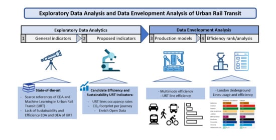
This paper introduces a methodology for assessing the efficiency and sustainability of an URT network based on large-scale data analytics consisting of four stages: (1st) EDA using state-of-the-art indicators; (2nd) EDA using new proposed indicators that deepen the analysis; (3rd) DEA using several original transport models, and (4th) rank transport modes and URT network elements according to efficiency measures, analyzing the results. Figure 1 summarizes graphically the methodology.
As URT systems, particularly in large cities, are a combination of complex interrelations, the proposed methodology aims at better capturing the most relevant efficiency and sustainability indicators to optimize transport infrastructures, from planning to real-time operation. Furthermore, as an additional outcome of this methodology, open-data repositories could be enriched with new data sources such as occupancy rates, queueing times, URT network elements capacities (e.g., stations) as well as CO2 footprints.
3.1. Exploratory Data Analysis (EDA) of URT Data
The first stage of the proposed methodology uses EDA for deriving state-of-the-art quantitative indicators [30]: network length, number of stations, the number of trains, the number of frequencies, the number of employees, the number of operated kilometers, and the number of passengers. This data is usually publicly available at transport operator level, useful for comparing operator’s efficiency, but it is more difficult to find at line level, limiting the analysis of the efficiency of rail network elements. However, thanks to big-data technologies (e.g., logging API requests/responses, queueing transport events, and web scraping) these indicators can be potentially estimated using models at a more fine-grained level. In the absence of data from operators (according to [28] only 9% of the research papers in this area has access to official data, generally open data) relying on big data is a much more scalable and cost-effective solution than ad hoc surveys. This approach will contribute to deepening the analysis of transport operators, thus increasing the limited number of research papers with city coverage (only 6% in [28]).
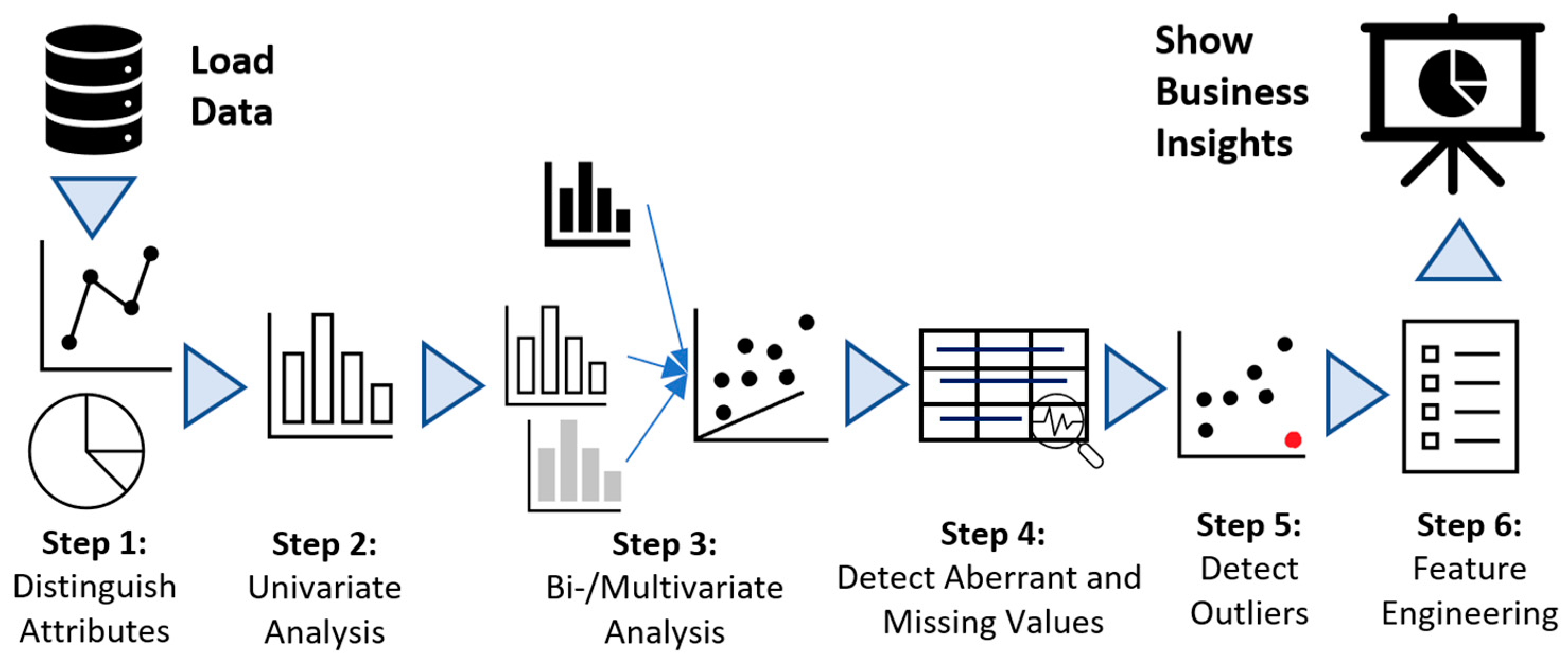
EDA, also known as Visual Analytics, is a heuristic search technique for finding significant relationships between variables in large datasets. Its simplicity and efficiency are key to derive insights from big data, in fact, it is usually the first technique when approaching data, particularly unstructured. According to Tufféry [42] EDA usually consists of six steps (see Figure 2) namely: (i) Distinguish/Identify Attributes; (ii) Univariate Data Analysis to characterize the data of the dataset; (iii) Detect Interactions Among Attributes performing bivariate and multivariate analysis; (iv) Detect and minimize impact of Missing and Aberrant Values; (v) Detect Outliers (further analysis or errors), and finally (vi) Feature Engineering, where features are transformed or combined to generate new features.
There is a large number of tools for performing EDA (50 of them are analyzed in [43]) with different functionalities to assist both with the identification of hidden patterns and correlations among attributes, but also with the formulation of hypotheses from the data and their validation. EDA can also be performed using R, python (used in our research work, programming ELTs—Extract, Load, and Transforms—followed by Datawrapper visualization) or any other programming language oriented to data preparation and exploration. Additionally, due to the geographical dimension of transport it is relevant that the tool includes Geographical Information Systems (GIS) support and a strong set of visualization capabilities.
3.2. Efficiency and Sustainability Key Performance Indicators (KPIs) for URT
The output of EDA is the estimation of state-of-the-art Key Performance Indicators (KPIs), as well as defining new ones based on large-scale data. For instance, new KPIs that can be defined are the number of trains per line that could be estimated based on the travel time and the rail frequencies. Moreover, another KPI, the number of passengers per line, can be estimated from the number of trains and the entry/exit numbers at the stations of a line. Finally, URT CO2 footprint can be estimated from the annual supply (in GWh) and the breakdown by source of the consumed electricity and their CO2 respective footprints.
Additional candidate KPIs that can be modeled after big-data sources are:
- Occupancy ratio: considering 100% occupancy ratio equals to all seated places plus 4 standing people per m2.
- Trains Per Hour (TPH): the number of trains that enter and leave a given station per hour, monitoring real-time traffic conditions.
- Travel time: from origin to destination, involving an URT journey.
- Excess Journey Time: is the additional time on top of scheduled time.
The definition, measurement, and analysis of the evolution of KPIs is key to improve the efficiency, security, convenience, and sustainability of existing URT. In fact, the public availability of these KPIs might support that personalized preferences for route selection can be expanded to, for instance, the occupancy rate, for ensuring the availability of seating space, CO2 footprint, or risk of an excess journey time higher than 10 min. Currently the preferences for route selection are quite rigid, the faster route, or manifest preference for a transport mode, although eventually passengers are considering additional factors, as seen when analyzing, anonymously, their routes using Wi-Fi data.
3.3. Data Envelopment Analysis (DEA) for Assessing Efficiency and Sustainability of Public Transport
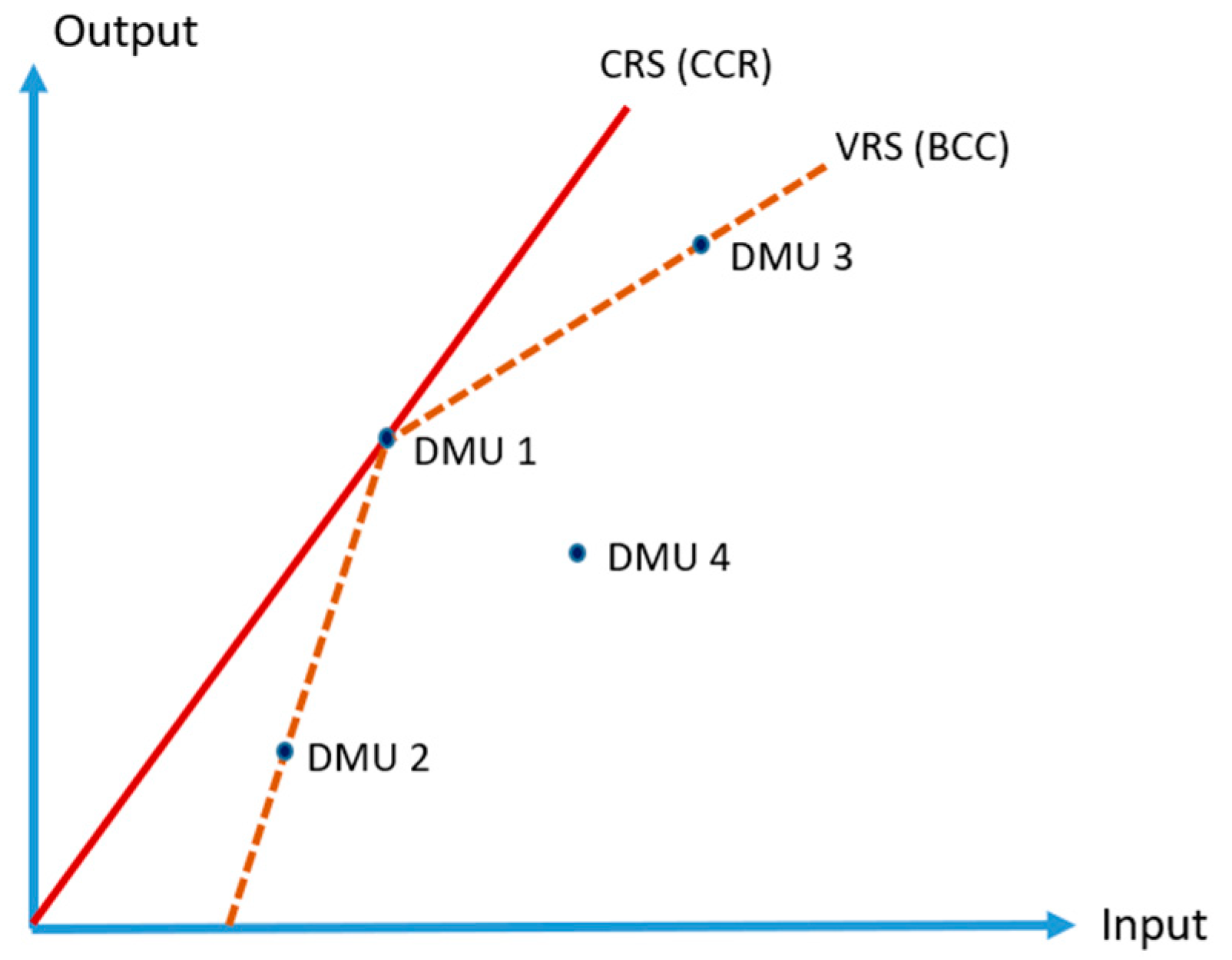
DEA is a non-parametric method to measure the performance of entities, called Decision-Making Units (DMUs). A DMU can be a factory, a bank branch, a hospital and, as in our paper, a transport mode, an URT line, or an URT station. The initial DEA models consider Constant Return to Scale (CRS or CCR for Charnes, Cooper, and Rodhes), which ignores the fact that different DMUs could be operating at different scales. In our scenario, it would not make any distinction between two URT lines, one with 6 stations and another with 60 stations. To overcome the drawback the Variable Returns to Scale (VRS or BCC for Banker, Charnes, and Cooper) mode [44] was introduced, ensuring that DMUs are only benchmarked against DMUs of similar size. Figure 3 presents an example of four DMUs and both CRS and VRS efficiency frontiers. DMU 1 is the only one in CRS efficiency frontier (the only efficient in CRS), maximizing the output/input ratio, whereas DMUs 1, 2 and 3 are in VRS efficiency frontier (the three are efficient in VRS, DMU 2 in low input values and DMU 3 in high input values). Further to VRS, a wide range of DEA models have been designed for measuring efficiency and capacity specializing the original models into different types of problems.
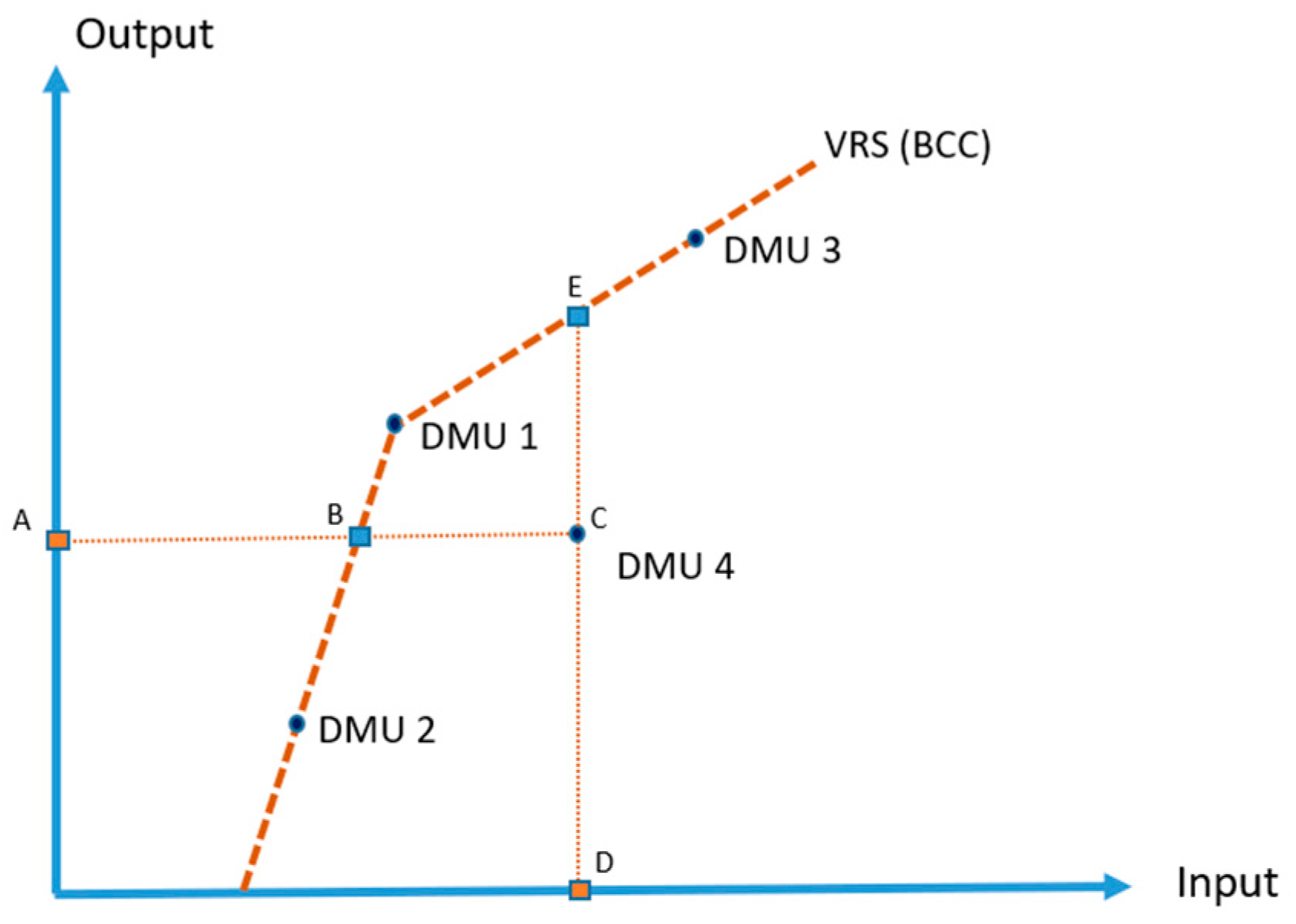
DEA models can be classified in either input-oriented or output-oriented models. Figure 4 shows an inefficient DMU (DMU 4 or C) to exemplify both approaches. Input-oriented efficiency is BA/CA. Output-oriented efficiency is CD/ED. With input-oriented DEA, a DMU computes the potential savings of inputs in case of operating efficiently (in Figure 4 reducing the inputs from C to B while providing the same output). In contrast, with output-oriented DEA, a DMU measures its potential output increase given its inputs do not vary (in Figure 4 increasing the outputs from C to E while using the same amount of input, D. If C were in the frontier, so C = B = E, the efficiency would be 1.
The bad/undesirable outputs, in our case CO2 emissions, have been treated as inputs reversing traditional DEA models [45,46]. This technique is based on the fact that undesirable outputs can be treated as inputs when there is a combination of undesirable and desirable outputs. The objective is to minimize the undesirable output, so considering it as input the function looks for its minimization.
A DEA model is a particular selection of inputs and outputs to analyze the efficiency of DMUs. In previous DEA assessments of transit lines, labor, capital, and energy have been used as inputs and vehicle-kms and passenger-kms have been used as outputs. In the absence of actual costs of labor, fuel/energy, and other operational expenses for individual transport lines, it is reasonable to assume that the cost of operating a line is related to its travel time, round-trip distance, and the number of stations/bus stops [35]. Additional, when alternative transport options are being considered, the cost is usually the single input whereas travel time savings, patronage (people for each transport mode), and car trips removed are outputs, as shown in [38], a study that implemented a constant returns of scale–output-oriented (CRS–O) model.
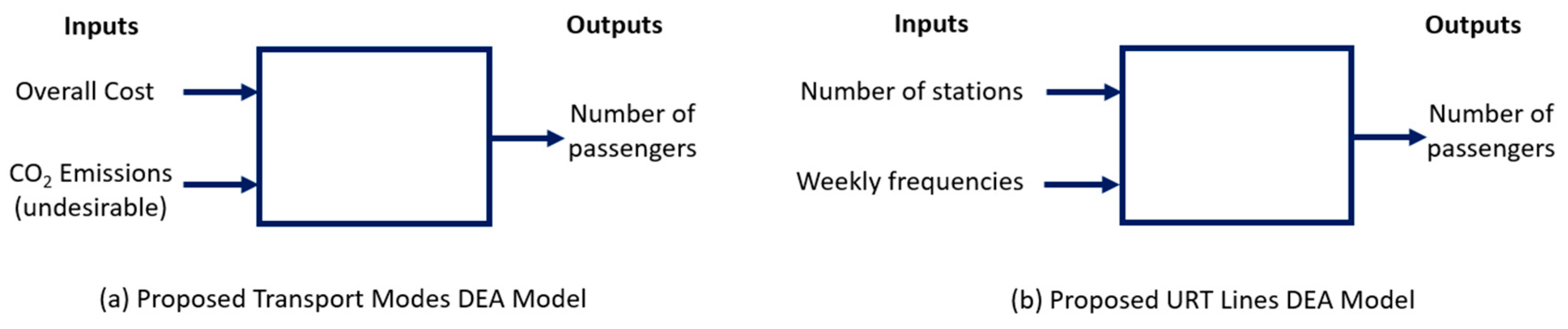
Figure 5 presents our candidate DEA models for: (a) assessing different transport modes from the traveler’s viewpoint (for route planning), and (b) analyzing URT lines from the operator/local authority perspective. The analyzed DMUs are the available transport modes (e.g., URT, bus, car, taxi, walking, and cycling) for the first model, and the available URT lines, usually in the range of 1 to 24 lines (e.g., New York has the highest number of metro lines, 24, followed by Beijing 23, Seoul 23, Shanghai 17, Paris 16, Moscow 14, and Tokyo 13). CRSs are considered for both models, in the transport modes model because route planning is generally used for one traveler (or a small group) and DMUs operate in the same scale, whereas URT lines, for a given URT network, are usually directly comparable.
The selection of inputs and outputs is especially relevant in this scenario due to the large number of available variables and the modest sample size. Following the cardinality constraints introduced in [39], the recommended number of variables for these two CRS models is 3 (in case of considering VRS it would be 2). The selected variables depend eventually on EDA on the available data; however, a tentative output is the number of passengers, and the models can be considered input-oriented, designed for minimizing inputs when moving a given number of people.
In the first model CO2 emissions, an undesirable output, have been treated as input, as already mentioned, while considering the overall cost the only true input [38]. Here, as the model is from the passenger viewpoint, the overall cost is the transport fare (or the direct costs incurred) plus the monetary value of the passenger time. As most of the mobility is associated with commuting to work, the passenger time value can be estimated at the cost of unskilled working time, although this can be configured on a per-passenger basis for personalized route planning. The selection of these two inputs, which combined with the output reaches the recommended number of variables (3), is original, selected after using EDA on the available data, which contrasts with state-of-the-art indicators for route planning such as travel time and fare cost.
With regards to the URT lines model, two tentative inputs, subject to change due to EDA conclusions on the available data for a given URT network, are considered: (1) the number of stations per line as estimate of the capital costs (CAPEX); and (2) weekly frequencies as operating costs (OPEX).
The related literature in public transport generally uses the actual investment as CAPEX; however, when considering URT lines it is neither directly disaggregated per lines, nor comparable across the time (e.g., 20th century vs. 21st century URT lines). The number of stations per line has been selected as input due to the wide availability of this KPI, although generally indirectly, derived from the longest URT route obtained from online route planning/maps services and applications. The line length, although it is a more popular metric and it is also widely available, has not been selected after EDA on the available data (data sourced from [47]) as long lines usually have generally lower investment due to a higher ratio of above-ground to underground construction, especially in suburban areas where distance between stations tend to be higher. In fact, in [47], a reference paper in CAPEX in Urban Rail only considers costs per kilometer, a state-of-the-art KPI, which shows a higher variability than the cost per station (e.g., in 16 European URT projects, after discarding 3 outliers, the cost per kilometer ranges from 26.7 to 88.3 M USD$, whereas the cost per station ranges, for the same projects, from 39.4 M to 83.1 USD$), with lower standard deviation. Additionally, stations have a share of 25–30% of the infrastructure costs, which favors the selection of the number of stations versus line length as CAPEX.
Regarding OPEX inputs, the related literature in public transport generally uses the price of labor and the price of fuel. However, they are not particularly useful for comparing different lines within the same URT system, as they are set at the operator level. Labor and energy consumption can vary per line, although this level of detailed data is generally not available. Nevertheless, a variable directly related to OPEX that is generally available per line is the number of weekly frequencies. EDA on route planning data shows different patterns for weekdays and for weekends, so the week is the selected period. This input, in combination with the number of stations (the other input), are the selected variables for this DEA model after EDA on publicly available data from URT systems.
The shortlisted inputs (e.g., number of stations and weekly frequencies) have a relevant positive correlation with most of the state-of-the-art inputs, such as the line length, labor force, and number of URT cars, as shown from EDA on [47] and validated in Section 4 (e.g., using LU lines key parameters), thus making it a highly representative selection, with higher discriminatory power and simplicity thanks to minimizing redundancy. Furthermore, the shortlisted inputs are directly obtained from route planning services and applications (e.g., Apple Maps, Bing Maps, Google Maps, and services such as Rome2rio.com that, as of today, includes worldwide 176,885 rail lines from 4151 operators), significantly easier than collecting data from other sources, some of them not available publicly. Finally, in case of availability of data, our candidate inputs for a more representative model would be car capacities, consider line branches, and breakdown passengers into time bands (a.m./p.m. peak versus off-peak). The selection of these additional candidate inputs, which add relevant information about URT efficiency, is one of the outcomes of the previous step, defining new indicators from EDA.
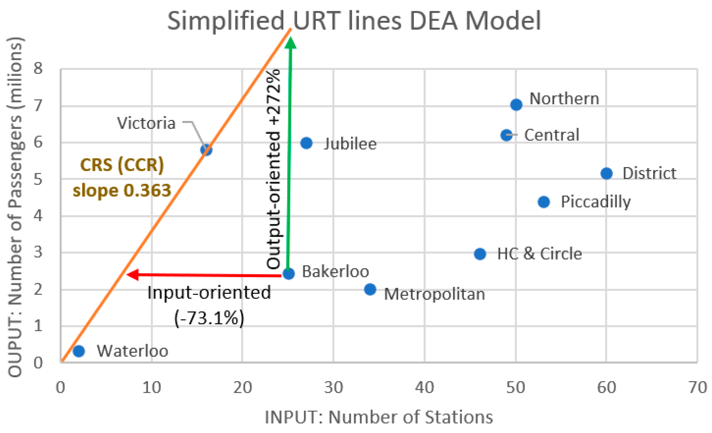
These DEA models have been computed using the solver software that comes with the reference DEA book by Cooper [6]. To illustrate DEA concepts this subsection concludes with an example of DEA analysis, computing the efficiency of London Underground (LU) lines, the use case to validate the proposed models, using for clarity purposes a simplified URT lines DEA model, with a single input, the number of stations, and a single output, the number of passengers. Table 1 summarizes the input and output data, as well as the results provided by the solver. As there is a single input/output the resolution is direct.
The DMU Victoria maximizes the production function (weekly passengers per station), 363,000, so it scores 1. Compared to the first DMU of the list, Bakerloo, with 98,000 passengers per station, 26.9% of 363,000, thus scoring 0.269. This is a CRS model, similar to the two proposed models, so the production function is the same for all DMUs, not varying at scale (as for VRS). Since there is a fixed number of stations, the key parameter is the number of passengers that maximizes the efficiency for each line, so the model has been computed as output-oriented. In fact, the highest ratio, 363,000 passengers per station, has been used to compute the projection of passengers, presented in Table 1, as well as the difference between the projection and the actual line passengers. Thus, for Bakerloo, ranking 6th in Efficiency, the projection is 9.08 million passengers, +272% over the actual number of passengers, 2.44 million passengers. Alternatively, models can be computed following an input-oriented approach, thus minimizing the required number of stations to achieve the maximum ratio. Thus, for Bakerloo line, it would need to carry 2.44 million passengers with 6.7 stations (2.44/0.353), which is 73.1% less stations (1 minus its efficiency score, 0.269).
Figure 6 represents graphically the 10 DMUs (URT LU lines) using their coordinates (number of passengers as y axis and number of stations as x axis). The production function, CRS, achieves its maximum value for Victoria, thus scoring 1 in efficiency. Please note that the CRS function starts at the origin (0,0). The remaining DMUs score below 1, depending on its ratio passengers/station compared to the optimal. The least efficient is Metropolitan, graphically it can be seen that it has the minimum slope to the origin. The figure also helps to understand how to measure inefficiency. Using Bakerloo as a sample, on the one hand, for input-oriented, the CRS optimal function requires 73,1% less stations (6.7 stations) for moving 2.44 million passengers. On the other hand, for output-oriented, CRS optimal function can move 9.08 million passengers, +272%, with 25 stations.
3.4. Ranking DEA Models URT Lines According to Efficiency Indicators
The fourth and later stage of our methodology is to rank both transport modes and URT lines using the results of the DEA models. The efficiency of the transport models, from the traveler’s viewpoint, can be used for personalized route planning, suggesting different transport modes depending on the time band, the travel distance and the user preferences (e.g., their own estimate of its value of time, and the usage of new mobility solutions such as private electric scooter, or bike/moto/car-sharing).
With regards to URT lines, ranking them according to their efficiency scores instead of less sustainable metrics, such as the number of car-kilometers or the increase in the number of passengers, contributes to align the public transport operation with sustainability goals. In fact, the most efficient URT lines will be those with a reduced number of stations and weekly frequencies that are able to transport more passengers. This model/rank can be complemented with the personalized route planning, as the frequency between URT services could be modified (increased/decreased) up to a point where URT is still the preferred transport choice.
3.5. Big Data and Sustainable URT
Public transport services, particularly URT systems, due to the economies of scale, are among the most efficient activities. However, they confront huge initial capital investments, and variables such as the number of stations, length, speed, are determined by this capital investment. Therefore, it is key to characterize their efficiency and sustainability, key to monitor its management.
Big data can gather, store, and process large amounts of heterogeneous, large-scale data to assist regulators, cities, transport operators, and travelers to improve the efficiency, regulation enforcement, and sustainability of their mobility solutions. So far route planning (e.g., Masivo model [48]) and public transport timetable optimization [49] are based on simulation models which can greatly benefit from the incorporation of big-data analysis into their models. Additional big-data applications are personalized route planning and smart taxation (based in the polluters-pay principle) such as dynamic tolling depending on the specific CO2 footprint of cars and their usage (kilometers) in city centers, where air quality has one of the highest impacts on people’s health.
4. Case Study: Efficiency and Sustainability of London Underground (LU)
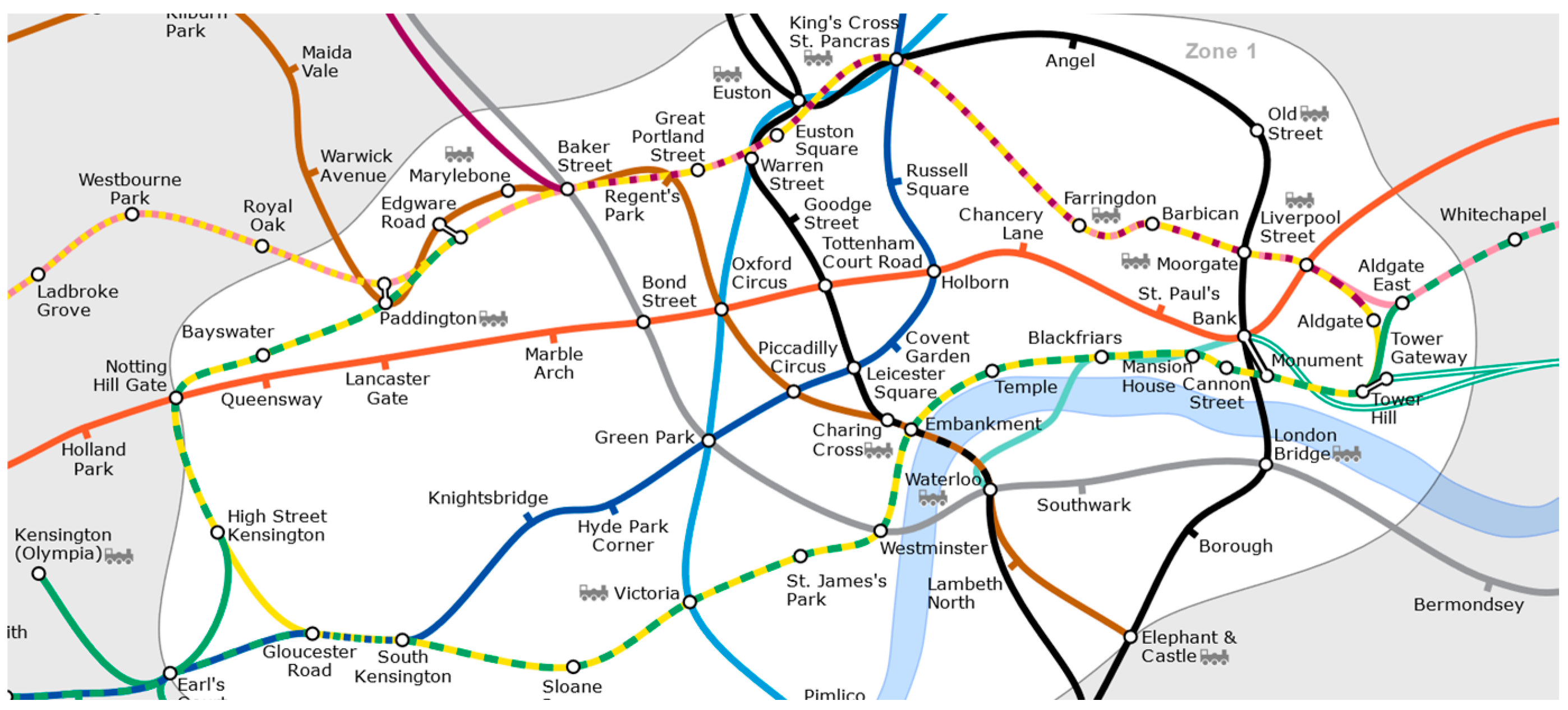
This section presents the validation of the proposed methodology by analyzing the efficiency and sustainability of a reference URT network, the LU, selected because of the complexity of its network (3 million daily journeys, served by 540 trains across 10 lines covering 402 Km and 263 stations. Figure 7 presents the core of the LU network), and its open-data NUMBAT database (see Appendix A), one of the few publicly available and successful [50] datasets on URT.
NUMBAT provides entry/exit/interchange passenger count for 263 stations and the number of trains per station every quarter hour. Additionally, it provides a 263 × 263 origin station–destination station matrix, covering all journeys and the annualized number of passengers for each line. However, NUMBA data is based on real data, but it is not real data. It is the output of a synthetic model used to research LU usage and travel patterns. Moreover, it assumes a perfect train schedule being operated and that all passengers board on the first train arriving at the station. This synthetic model is based on sampling real data from smartcards and gateline entry/exit totals for each station. Data is provided in quarter hours, grouped also by time bands (Early 3–7, AM Peak 7–10, Midday 10–16, PM peak 16–19, Evening 19–22, Late 22–3). Finally, data has been provided in a differentiated way for Fridays, Saturdays, Sundays and for the average of the remaining days (from Monday to Thursday).
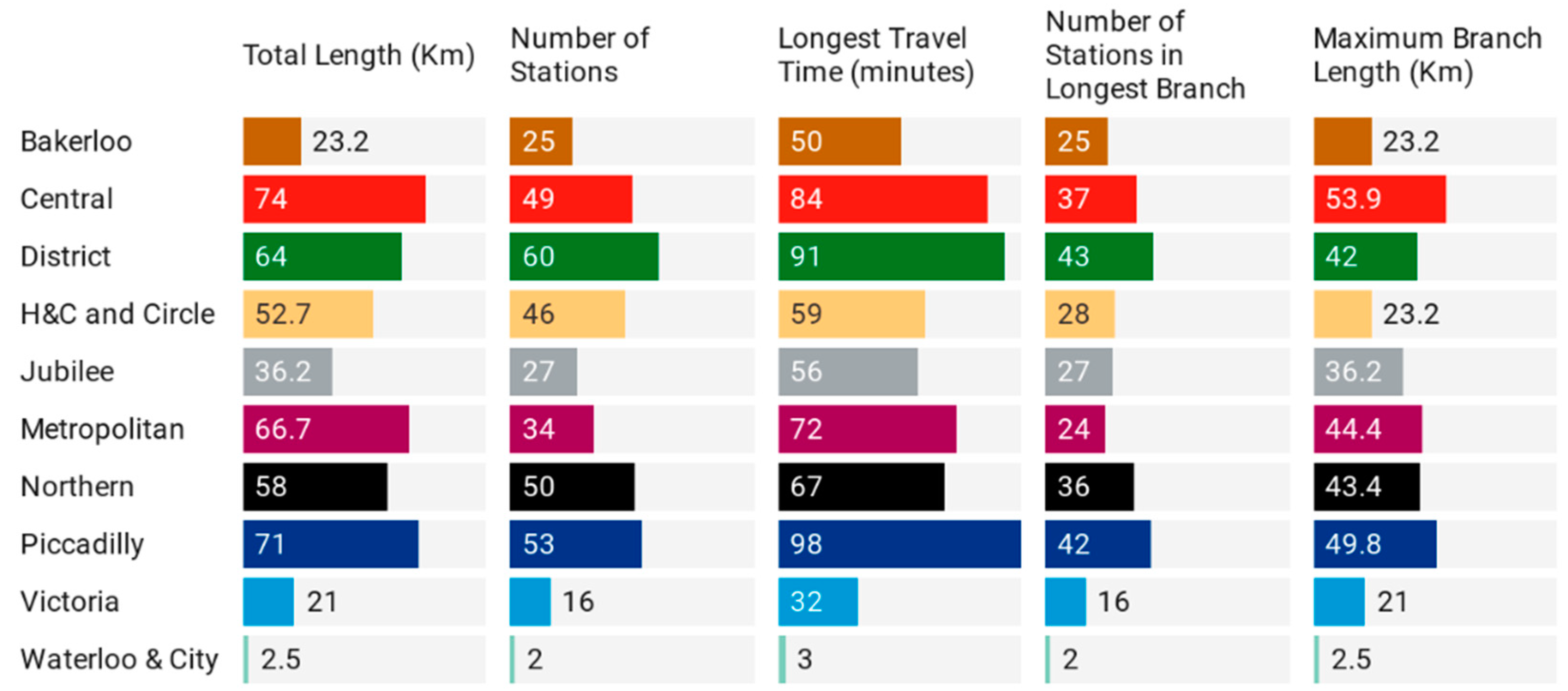
As NUMBAT is quite limited (e.g., there is no information about schedules and LU lines, neither descriptive, nor the stations that belong to a line nor the capacity of the trains), we have extended this database with four major data incorporations: (i) train schedules; (ii) a table that relates lines with all their stations; (iii) a table that relates lines with their capacity (seated plus standing at 4 passengers per m2), with data collected from TfL website (TfL open data does not include this data); and (iv) include GPS location for all the stations, obtained from Open StreetMap [51]. See Appendix A for further details. Figure 8 presents some key descriptive metrics of LU which are not originally available in its open-data repository.
4.1. Assessing the Efficiency and Sustainability of LU Using EDA
The first step of EDA is to distinguish attributes. Table 2 gathers LU key attributes: 3-letter LU line code (in the same order as Figure 8); the longest travel time in the line, it is the average scheduled time of the longest service, usually from the first until the last station of the line; and the length, in kilometers and stations, of the longest route. Additionally, the table contains the scheduled weekly LU frequencies at the station with the highest number of frequencies (usually stations at the middle part of the line), and the weekly passengers per line. A passenger counts as one passenger for each of the lines traveled. On average, a LU passenger uses 1.6 lines per journey (42.4 Weekly passengers in lines and 26 million weekly LU journeys).
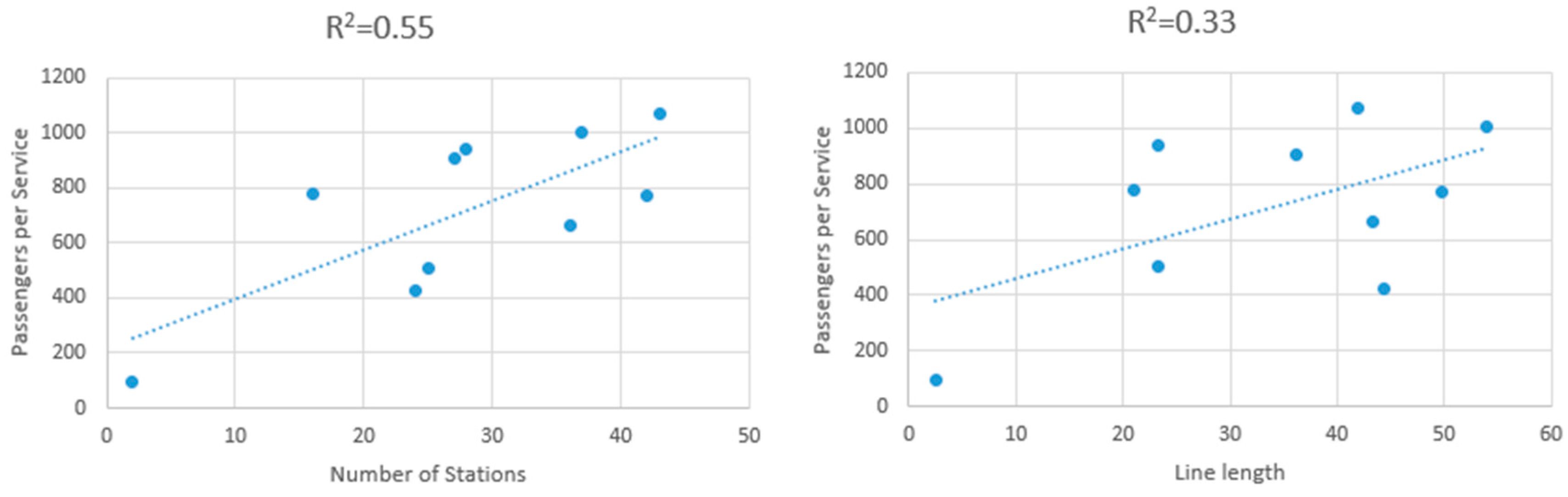
The next parameters in Table 2 are metrics/KPI derived from the previous data. Figure 9 presents the scatter plot graphs of the number of passengers versus the number of stations (left), two variables that correlate positively with R2 = 0.55 (the higher the number of stations, the more travelers it captures). Figure 9 also shows the number of passengers versus the line length (right), with R2 = 0.33 (a long LU line might be reaching areas with less population density, so this correlation is weaker than the previous one). Additional parameters are the average number of passengers per service and station (included as it contributes to explain the variability with R2 > 0.5, discarding the line length). Finally, Speed, in terms of km per hour and minutes per station is presented to illustrate key metrics of LU operation. Based on these analyses, two parameters, the number of stations of the longest route and the weekly frequencies, have been selected to be used in the second phase of the proposed methodology, efficiency scoring using DEA.
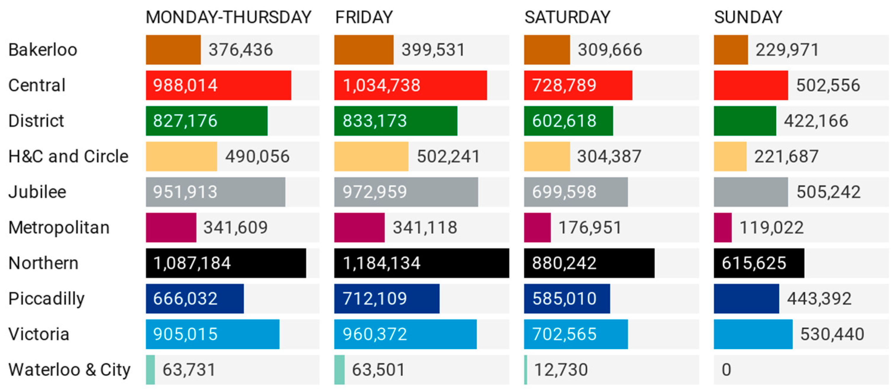
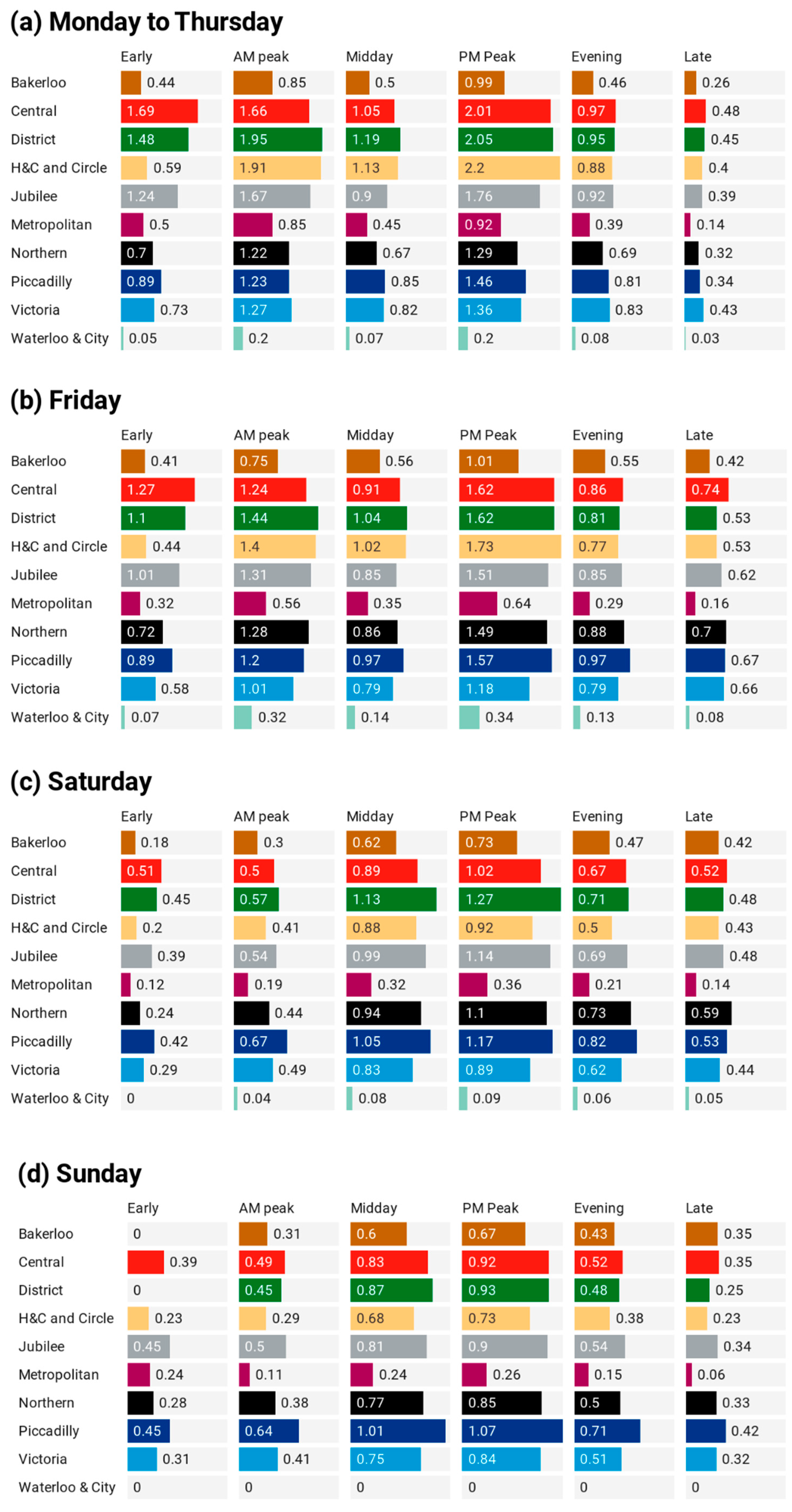
So far, the analyzed metrics are average numbers, not considering a relevant source of variability, the day of the week and especially the time band. Figure 10 presents the number of passengers per line and day of the week. The dataset provides an average number from Monday to Thursday. Fridays, except for the Metropolitan and Waterloo & City lines, is the busiest day, whereas Sundays is the day with the lowest number of passengers.
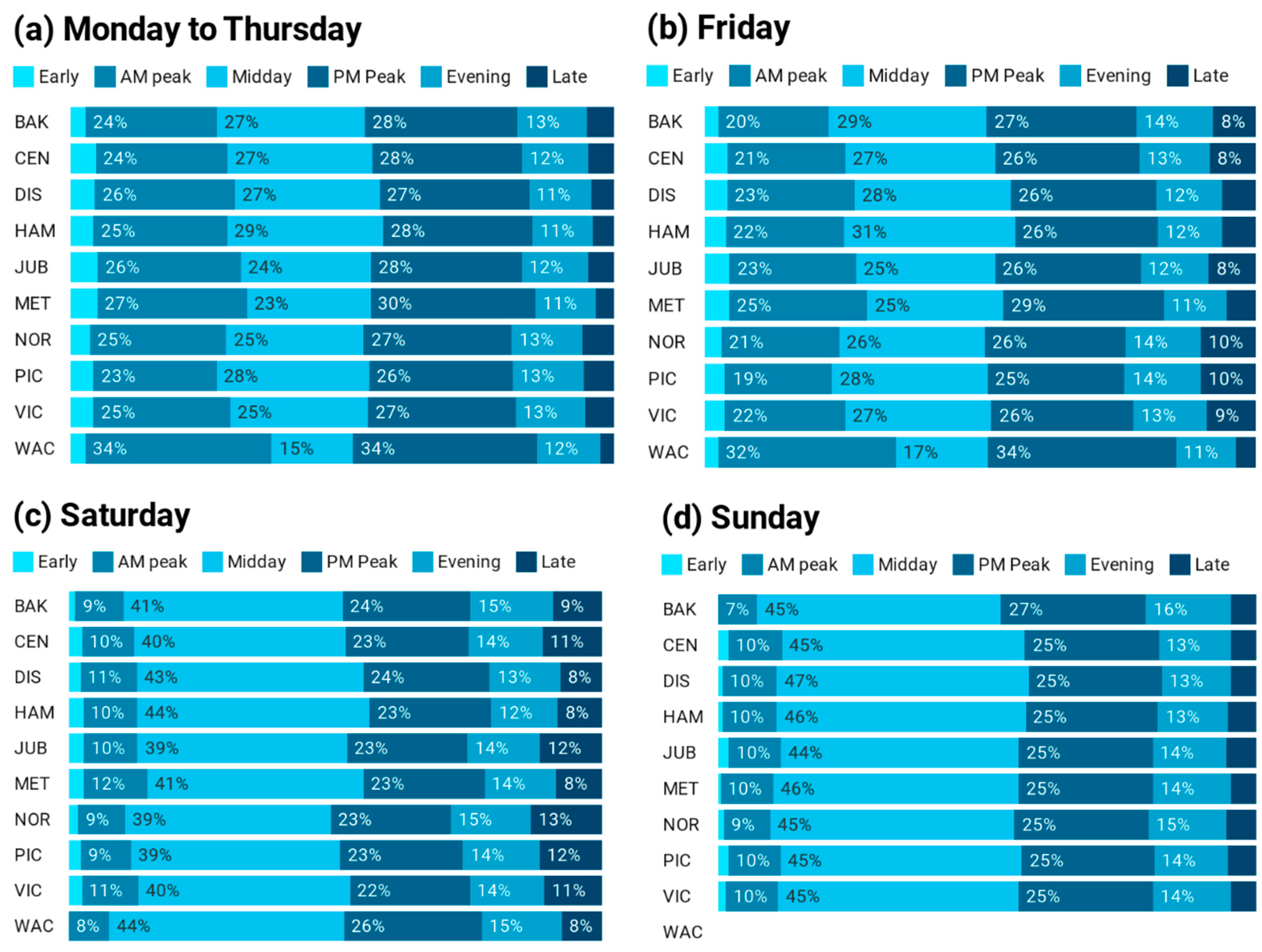
Figure 11 presents the distribution of passengers per day of week and time bands (Early 3–7, AM Peak 7–10, Midday 10–16, PM peak 16–19, Evening 19–22, Late 22–3). AM and PM peak hours (3 h each) concentrate most of the use from Monday to Friday, whereas Midday (6 h) is the preferred time band for weekend passengers. WAC (Waterloo & City) only operates from Monday to Saturday and has the highest use during Monday to Friday peak hours. Late traffic is higher on Saturday and also Friday, which motivates the different traffic pattern of Friday versus Monday to Thursday, and the higher number of passengers of Friday than Monday to Thursday (except MET and WAC lines, see Figure 10).
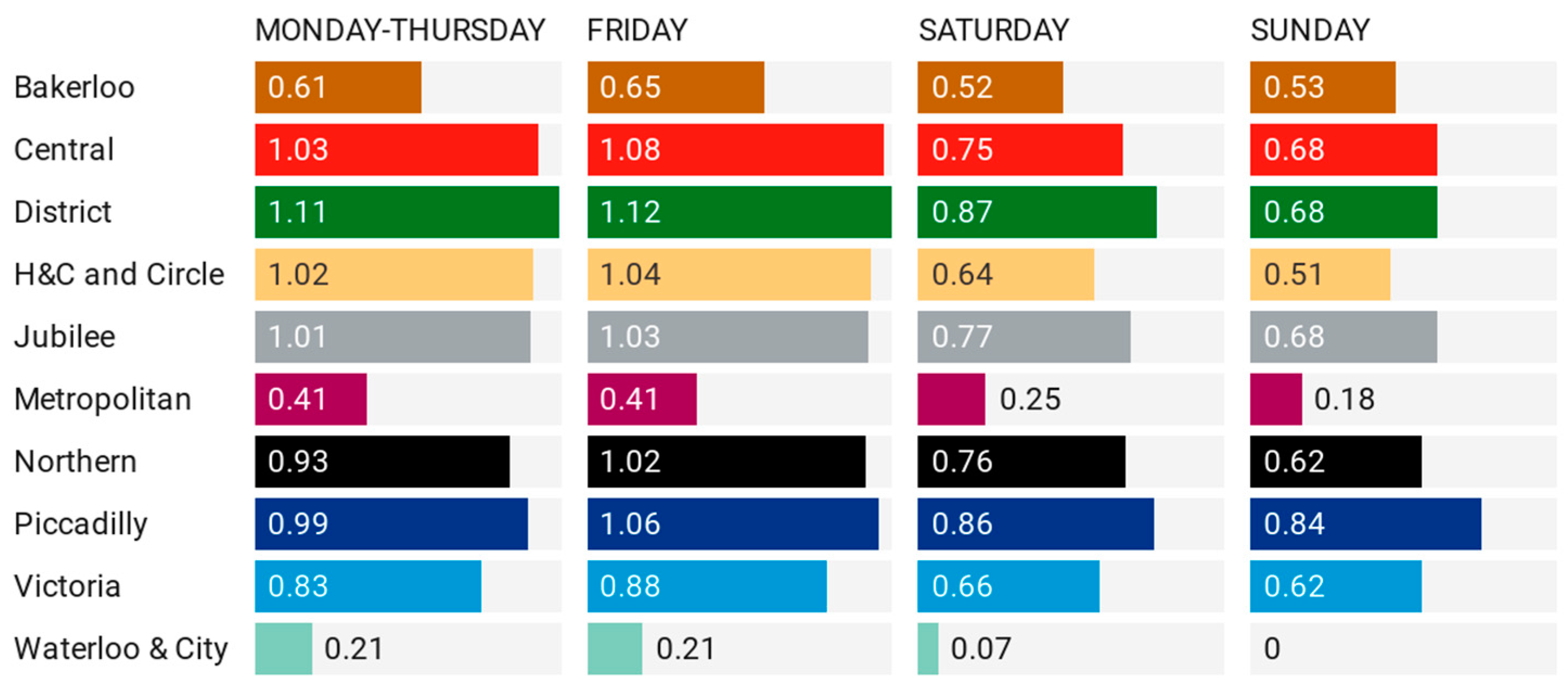
A new metric, occupancy rate (usually not reported by URT operators), has been computed dividing the number of passengers by the capacity of the line by time band. To compute this KPI the underground capacity has been considered (seated spaces plus 4 standing passengers per m2, see Appendix A). Figure 12 presents the occupancy rate, sometimes higher than 1 (e.g., Central and District lines). This means that a train, when going from the beginning to the end of the line, can move more passengers than its theoretical capacity. This is possible because these lines, Central and District, have branches and multiple exchanges with other lines, so each seat/standing space can be occupied by more than one passenger per service. A model that estimates the maximum capacity of a line based on an origin–destination trip matrix has been already suggested [52]. However, in our work we will capture these differences in the DEA efficiency model, without providing specific weights to the behavior of line travelers. However, the availability of actual origin–destination data (not the model-based NUMBAT dataset) would increase the interest of this research.
Figure 13 presents the occupancy rate by line, day of the week, and time band. On the one hand, the highest occupancy rates are in PM peak band (4–7 p.m.) from Monday to Thursday, particularly in Central, District and H&C and Circle lines, with rates over 2. As mentioned, on average a LU travel involves 1.6 lines, and these three lines cross Central London, so they might be capturing a relevant number of travels from/to an exchange to another line. In fact, the most crowded line, H&C at PM peak time, has lower traffic at Early time band (before 7 a.m.), which means that is a line close to weekday main destinations (Central London). On the other hand, the occupancy rate of Metropolitan and WAC is the lowest.
Next step is to explore the occupancy rate between two contiguous stations, to characterize the real occupancy rate experienced by travelers. The number of station links is the number of stations minus one for each line, thus 352 station links. The most relevant information analyzing occupancy rates are those extreme values, the lowest and highest, particularly the latter. Figure 14 shows the most crowded station links at the quarter hours with the highest occupancy rates during AM peak (left), 8:30–8:45 a.m., and PM peak (right), 5:30–5:45 p.m. These numbers have been derived from our dataset, combining passengers, line schedules, and line capacities. However, these are estimates as the real flow of passengers and train delays are not publicly available. As the objective of this paper is to characterize the efficiency and sustainability of LU, EDA finishes with the analysis of occupancy rates of stations links, relevant for assessing that the LU carriages theoretical capacity (with 4 standing people per m2) can be considered its maximum capacity.
4.2. LU Additional KPIs
TfL considers additional LU KPIs in its reports [53], focused on service provision, reliability, and journey times, such as the percentage of scheduled kilometers operated (95.8% of the 88.7 million kilometers scheduled), and the excess journey time, and the average delay or (4.6 min, 11% of the average journey time which is 41.6 min). The average delay is formally defined as excess journey time, the additional time on top of scheduled time for access/egress/interchange, platform wait time and on train (the latest figure is 4.6 min for LU for 2018/2019 (table 12.5 in [53]). TfL has reduced the excess journey time since 2008/09, from 6.6 min to 4.6 min by increasing the frequency of the services around 20% higher.
Finally, from the attributable CO2-equivalent emissions of operating LU (372,000 tons) and 12 billion annually passenger-km [53], a footprint of 31 g of CO2-equivalent has been estimated by us. Previously, TfL released, outside of the open-data repository, its CO2 footprints with out-of-date higher estimates [54]. Additional non-official estimates exist [55,56], although also out-of-date. Although the number of operated kilometers raised a 20% over the last 10 years, the CO2 footprint has decreased far more than 20% (LU operates with power and UK National Grid has been reducing more than 20% its CO2 footprint during this decade). Thus, LU is more sustainable than a decade ago, and more sustainable than buses (97% fuel-based), which have and 90 g CO2 footprint per passenger per km (480 million vehicle-km, 4.45 billion passenger-km, and an average CO2 emission of 822 g/km per vehicle, accounting for around 400,000 CO2 tons).
4.3. Assessing the Efficiency and Sustainability of London Transport Modes Using DEA
This subsection presents the efficiency of the proposed DEA models, first transport modes, and second URT lines.
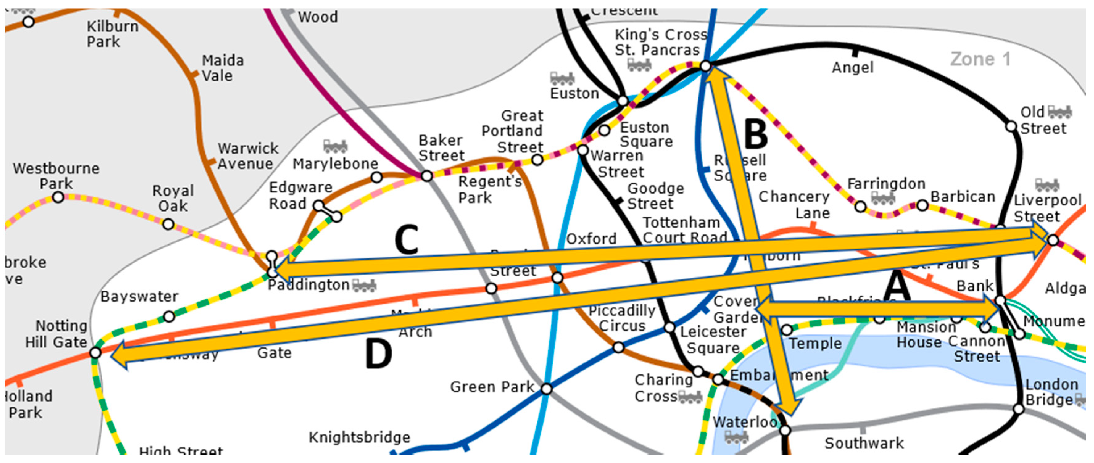
Figure 15 presents four routes to evaluate five transport modes (LU, bus, car/taxi, walking, and cycling), and potential combinations of these five transport modes, in Central London, from the shortest to the longest: (A) Bank–Covent Garden, (B) King’s Cross St. Pancras–Waterloo, (C) Paddington–Liverpool Street, and (D) Notting Hill Gate–Liverpool Street. These are quite popular routes, connecting national rail stations, and commercial, leisure, and residential areas. However, apart from D, they are not directly connected via LU. Here the optimal route (minimizing travel time) for each transport mode, has been suggested by online services for multi-modal route planning (e.g., Rome2Rio, selected for reporting LU and bus distances and fares).
Table 3 presents the key parameters of the five analyzed transport modes for the Route A, and a sixth mode, the combination LU+bus. To be able to run DEA no missing values (or 0) are allowed, so it has been assigned a transport cost for cycling (0.20 GBP, the daily cost of an annual London cycle hiring subscription), and for walking (0.10 GBP per 2.4 km, an estimate of the cost of shoe wear). The estimated value of time is 12.00 GBP per hour, an estimate of unskilled pay rate in London, to consider the time factor. LU fare in Central London (Zone 1) is 2.40 GBP, and TfL Bus fare is 1.50 GBP. Costs are provided in the local currency. Moreover, for cycling and walking the additional physical activity has been also considered, estimating 1 g of CO2-equivalent emission per additional Kcal of energy. This number varies with the diet and weight of the traveler, although it is usually in the range 0.5–2 g CO2-equiv. per Kcal [57]. The additional cost of walking for a 70 Kg person at 5 km/h in a flat route has been estimated in 150 Kcal/h, and cycling at 15 km/h results in an additional consumption of 360 Kcal/h (these values are average of online calculators). Bus CO2 emissions are 90 g per passenger per km and LU footprint 31 g per passenger per km. Private car/taxi estimates are 120 g per km, the maximum for driving within the Ultra-Low Emission Zone (ULEZ) of Central London. The number of passengers has been set to 1. These and other values are being used only for illustrative purposes, they can be adapted for personalized route planning and personalized efficiency analysis. Nevertheless, to the best of our knowledge they could be valid estimates.
Computed DEA efficiencies for Route A are 100% efficiency for cycling and walking, particularly for its lowest CO2 footprint, followed by the combination LU+walking (there is no direct LU link for Route A). Although bus+walking has the second lowest overall cost, its emissions are more than double the most efficient and it scores 64% efficiency. Car/taxi is the least efficient. DEA shows that the limiting factor for improving the efficiency of bus+walking and car/taxi is CO2 footprint, which can be seen graphically in Figure 16. Shifting from fossil fuel to electric transport can reduce emissions by 75% (according to CO2 footprint of electricity mix in the UK). Thus, bus+walking would reach the efficiency line whereas car/taxi would increase its efficiency significantly.
Table 4 presents the key parameters for Route B, in descending order of efficiency, from cycling, 100%, down to car/taxi, 21%. However, if 4 passengers go by car/taxi, CO2 footprint is the same (for clarity purposes we will consider the same), and the overall cost rises from 16 to 30 GBP, whereas for the other transport modes both CO2 footprint and costs are four times higher than the cost of one passenger. In this scenario, see Table 5, car/taxi jumps to the third efficiency position, rivaling with LU.
Table 6 presents the key parameters for Route C, in descending order of efficiency, from cycling, 100%, closely followed by LU, 94%. In this scenario the limiting factor is the cost. Considering 18 GBP per hour as time value then the fastest transport modes increase their efficiencies (LU rises to 100%, Car/Taxi to 40%), whereas slower transport modes reduce their efficiencies (Bus goes down to 52%).
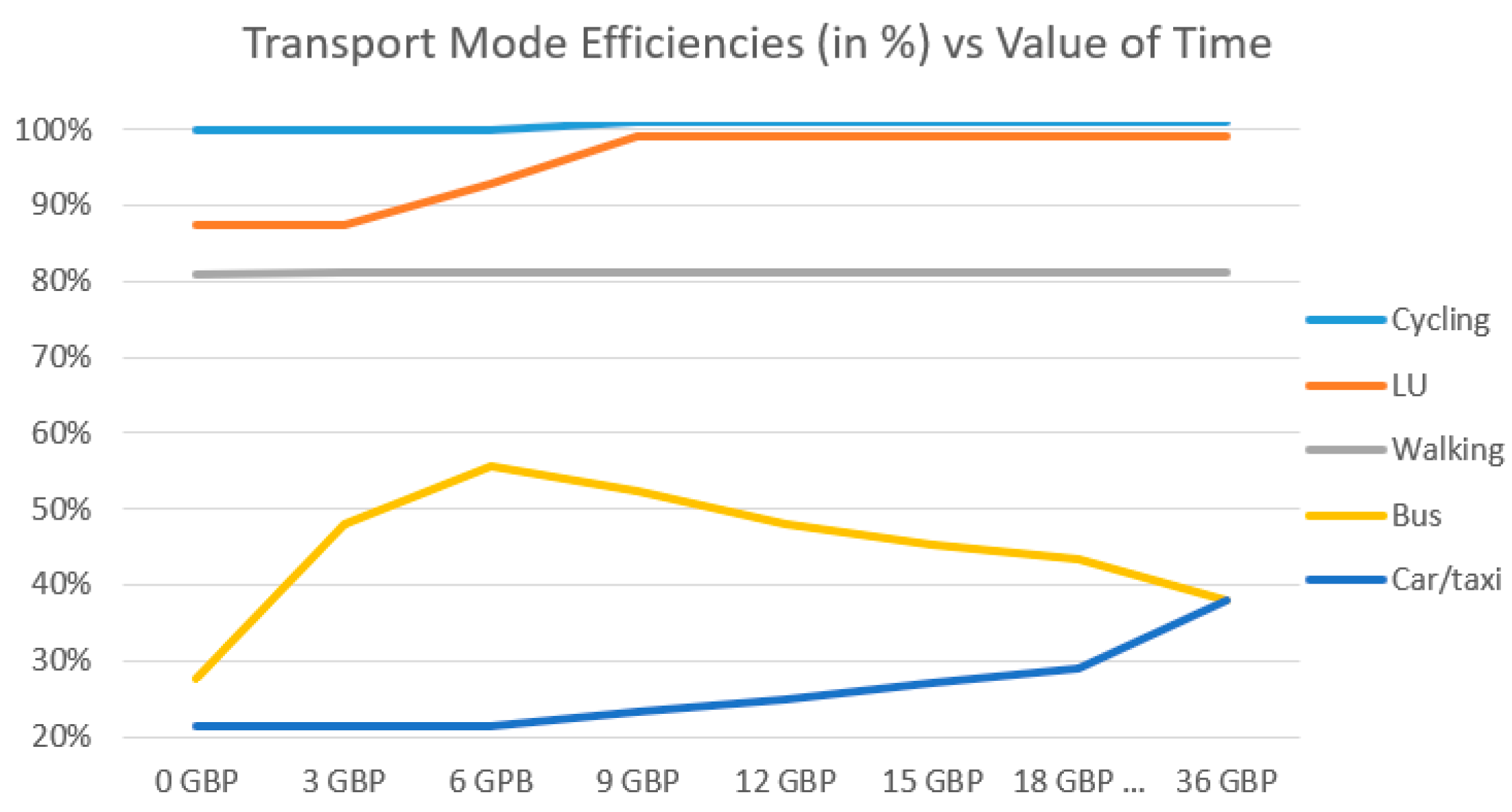
Table 7 presents the key parameters for Route D, in descending order of efficiency, where LU and cycling are both 100% efficient. LU has the lowest overall cost (Cycling has 27% higher cost, 7.60 versus 6.00) and the second lowest CO2 footprint (254 g., 14% higher than Cycling, the option with the lowest CO2 emissions with 222 g.). In this scenario both CO2 footprints and costs are the limiting factors. Thus, electrification of vehicles will have a limited impact if the overall cost remains unaltered. The main cost reduction would come from reducing even more travel times in buses and car/taxi. This might be feasible reducing traffic in Central London, for instance imposing higher restrictions to polluting vehicles in ULEZ.
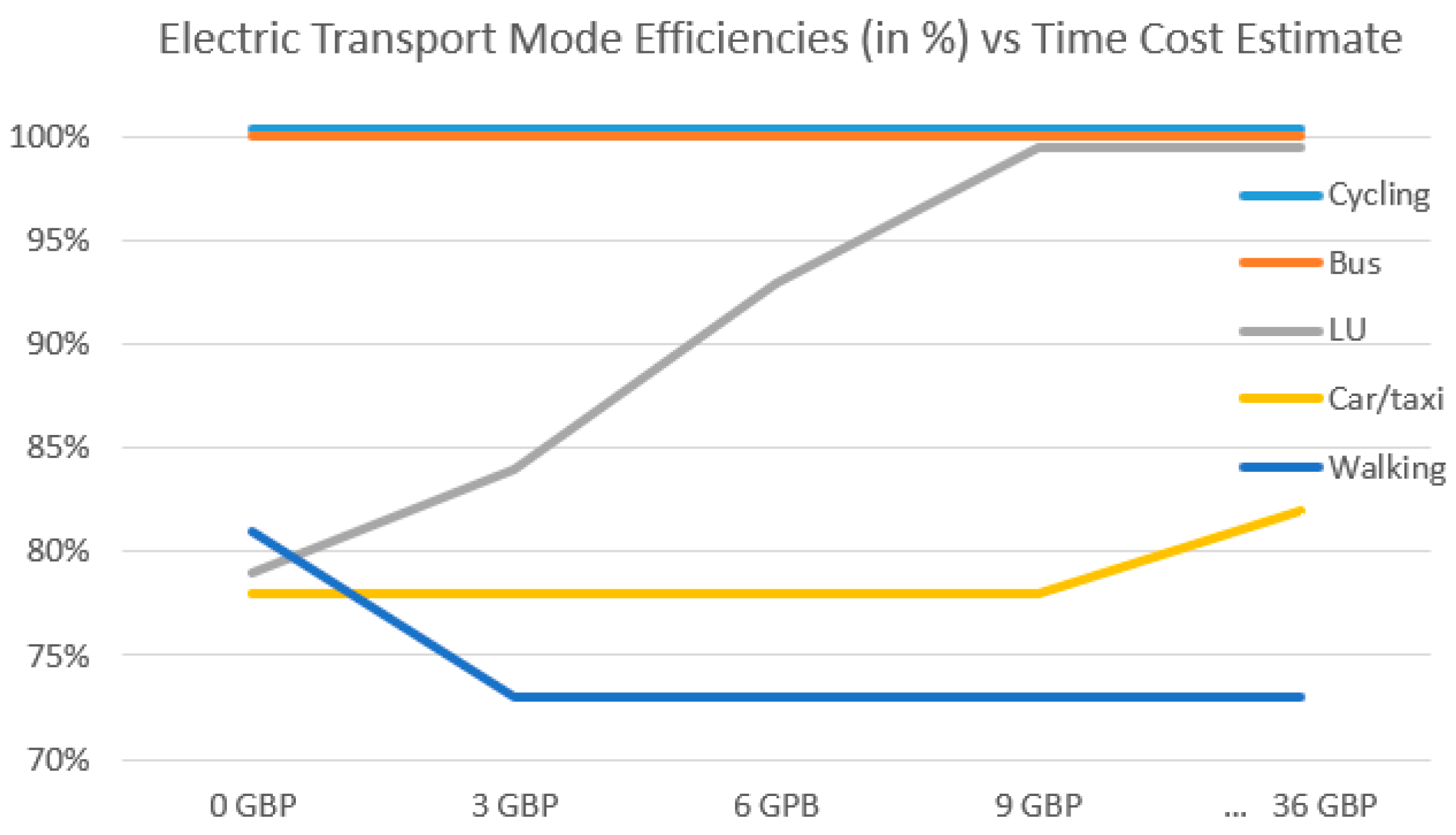
Figure 17 presents, considering the latter Route D, an analysis of the sensitivity of the value of time, the main factor impacting the transport mode efficiency. The range considered, from 0 GBP to 36 GBP per hour, shows that the fastest transport modes, Car/taxi and LU, gain efficiency as the value of time increases, slower for the Car/Taxi due to the higher transport cost of this mode. It is remarkable that walking, the slowest transport mode, keeps its efficiency due to its low CO2 footprint. Thus, a shift from fuel to electric vehicles, reducing the CO2 footprint by 75%, according to the energy generation mix in the UK, has been considered in Figure 18, also for Route D, together with a varying value of time. Now electric Bus is always 100% efficient, due to its low transport costs and low emissions, very similar to those of cycling, whereas LU, faster than LU and cycling but with a more expensive fare, is also efficient for passengers who value their time from 9 GBP/h on. In a scenario with electric cars/taxis this transport mode (Car/Taxi) is more efficient than walking from 1 GBP/h of value of time. As DEA is a relative (non-absolute) efficiency measure, improvements in some DMUs might impact the efficiency of other DMUs.
4.4. Assessing the Efficiency and Sustainability of LU Lines Using DEA
This subsection presents the DEA efficiencies of the URT lines model, a CRS model computed with the same DEA software solver as in the previous subsection.
Table 8 presents the key parameters of the ten analyzed LU lines, the two input parameters, the number of stations of the longest route and weekly frequencies, and the output, weekly passengers. Then the efficiency, ranging from 44% for the Metropolitan line to four 100% efficient lines (Central, District, Jubilee, and Victoria line). In addition, finally, four KPIs considered in EDA to characterize and compare LU lines. Although DEA is a non-parametric technique, so efficiency is not a linear combination of the inputs, it looks as if the best performers are those lines with the highest average passengers per service, the highest passengers per service and station, and the highest speed. WAC efficiency (46%, 9th) is limited by the weekly frequencies, with just 426 weekly frequencies (87% lower than the current number), retaining the number of passengers, it would be 100% efficient. The rest of the inefficient lines, those scoring below 100%, are limited both by the number of stations and the weekly frequencies. Table 9 shows the optimal projections of the inputs of the LU lines.
An efficient line would maximize the number of passengers with the lowest number of stations (proxy variable of the capital expenses, CAPEX), and the lowest weekly frequencies (proxy variable of the operating expenses, OPEX), an analysis in tune with previous works [30]. However, to increase the efficiency, closing stations is not an option. URT management can only influence operating expenses, reducing/increasing the weekly frequencies. Thus, the efficiency of a LU line will increase if reducing a given percentage the number of weekly frequencies (e.g., 10%) the number of passengers reduces significantly less than the reduction of the frequencies. Further analysis of real transport data, actual number of passengers and actual schedule of LU trains, will help to understand the relationship between frequencies and the number of passengers of a line, particularly in such a complex network as LU, with multiple exchanges and different lines sharing the same rail section/station links.
Table 10 presents an alternative DEA model with two additional input variables, the longest travel time, and the longest length in km. The new ranking that comes out of this extended model only interchanges positions 8th and 9th, as the new variables are highly correlated with the previous input variables. Thus, now WAC ranks 8th and BAK ranks 9th as the new model favors the short length and travel time of WAC, although BAK also increases its efficiency.
Finally, Table 11, Table 12 and Table 13 present the efficiency of the proposed URT lines DEA model (the original with 2 input variables) using the data, frequencies, and passengers, for AM, Midday, and PM peak time bands, from Monday to Thursday, respectively. Efficiency results for the mentioned time bands (bands of 3, 6, and 3 h, respectively) are in tune with overall line efficiencies presented in Table 8. However, some differences arise, such as WAC is the 7th in efficiency during peak times, but the 10th during Midday. WAC connects a national rail station and transport hub, Waterloo Station, with Bank tube station, in the heart of the financial area in the City of London. Therefore, its traffic pattern shows more activity during AM and PM peak hours. Moreover, VIC is the only line 100% efficient in the three time bands. Finally, except for WAC, LU lines score similarly across the analyzed time bands.
5. Conclusions
This paper has analyzed the efficiency and sustainability of URT using EDA and DEA. The main contributions of this work are: (1) propose and compute new indicators for EDA of URT sustainability and efficiency (e.g., occupancy rate by URT line, station links, and time band, and CO2 footprint per journey); (2) design and propose a methodology for DEA performance assessment based on the selection of input and output variables using EDA on publicly available data; (3) develop two original DEA production models, the first one for characterizing the sustainability of different transport modes, and the second one for measuring the efficiency of URT lines; (4) validating the methodology with open data from TfL and online services; and (5) ranking URT against other transport modes and analyzing DEA efficiency scores of URT lines.
The main conclusions of the paper are: (1) EDA plays a key role analyzing URT efficiency and sustainability indicators, as well and defining new indicators; (2) DEA variable selection can be done in a semi-automated and repeatable way relying on EDA; and (3) DEA is a simple and straightforward non-parametric technique to score multiple transport modes and URT lines efficiency to monitor, understand, and improve its management, even focusing on time bands and URT line sections for the latter scenario.
To sum up, the introduced big-data-based methodology supports the advance of efficiency and sustainability in public transport, particularly in URT, through disseminating data, KPIs, and assessments based on them. Thus, both operators and travelers alike are encouraged to improve their decision-making, from transport network management to route planning, to meet the Sustainable Development Goal target of having a more sustainable transport by 2030.
Author Contributions
Conceptualization, G.L.T. and L.H.; Investigation, G.L.T. and L.H.; Writing—original draft, G.L.T.; Writing—review & editing, G.L.T. All authors have read and agreed to the published version of the manuscript.
Funding
This research was funded by the Ministry of Economy, Industry and Competitiveness of Spain, Project TIN2016-75845-P (AEI/FEDER/EU) and SNEO-20161147 (CDTI) and by Xunta de Galicia and FEDER funds of the EU (Centro de Investigación de Galicia accreditation 2019–2022, ref. ED431G2019/01, and Consolidation Programme of Competitive Reference Groups, ref. ED431C 2017/04).
Acknowledgments
The authors would like to thank CITIC and Project ref. ED431G2019/01 for supporting the Postdoc visit of Guillermo L. Taboada to Manchester Metropolitan University to develop part of the collaborative work presented in this paper.
Conflicts of Interest
The authors declare no conflict of interest. The funders had no role in the design of the study; in the collection, analyses, or interpretation of data; in the writing of the manuscript, or in the decision to publish the results.
Appendix A
The sources of data used in the study are openly available online on TfL open data site: https://data.tfl.gov.uk (accessed on 25 June 2020).
The main source of information is Urban Rail Passengers Count and Travel Flow Dataset (codenamed project NUMBAT), https://crowding.data.tfl.gov.uk, which is based on data, from smartcards (Oyster and contactless bank/NFC cards), gatelines, and automatic passenger counters and services from timetables, combined through a model to assign journeys to routes using generalized journey time. Data has been obtained during the autumn of each year (at the time of writing, autumn 2018 is the last one) and provides an average for weekdays from Monday to Thursday, and additionally data for Friday, for Saturday and for Sunday, each of them independently. Includes only aggregated data (~100 MB data annually). Additional information from TfL origin–destination dataset is described here: https://data.london.gov.uk/dataset/tfl-rolling-origin-and-destination-survey.
This dataset, published as open data using an open TfL license, provides:
- -
- Journeys per day by all URT modes in London, LU, London Overground (LO), DLR, Crossrail EZL, and London Trams.
- -
- – – Values for each 15-minute period of the day.
- -
- – – Number of passengers’ entries/exits at all stations.
- -
- – – Number of interchanging passengers at all stations.
This data has been enriched including GPS location for all the stations, obtained from Open StreetMap [51], (ii) creating a table that relates lines with all their stations (TfL open data does not include this table), and (iii) a table that relates lines with their capacity (seated plus standing at 4 passengers per m2), with data collected from TfL website (once again, TfL open data does not include this table). Table A1 presents LU lines and its associated train capacities.

Table A1.
LU train capacity per line as of 2018.
| Line Name | Capacity |
|---|---|
| Bakerloo | 851 |
| Central | 1047 |
| District | 1045 |
| H&C and Circle | 1045 |
| Jubilee | 964 |
| Metropolitan | 1176 |
| Northern | 752 |
| Piccadilly | 798 |
| Victoria | 986 |
| Waterloo & City | 506 |
References
- International Association of Public Transport UITP. Energy Efficiency: Contribution of Urban Rail Systems. Available online: https://www.uitp.org/energy-efficiency-contribution-urban-rail-systems (accessed on 25 June 2020).
- International Energy Agency. “Tracking Transport”. Available online: https://www.iea.org/reports/tracking-transport-2019/rail (accessed on 25 June 2020).
- Sustainable Mobility for All (Sum4all). Global Mobility Report 2017. Available online: https://sustainabledevelopment.un.org/content/documents/2643Global_Mobility_Report_2017.pdf (accessed on 25 June 2020).
- Tukey, J.W. Exploratory Data Analysis; Addison Wesley: Reading, MA, USA, 1977. [Google Scholar]
- Charnes, A.; Cooper, W.W.; Rhodes, E. Measuring the efficiency of decision making units. Eur. J. Oper. Res. 1978, 2, 429–444. [Google Scholar] [CrossRef]
- Cooper, W.W.; Seiford, L.M.; Tone, K. Data Envelopment Analysis; Springer: New York, NY, USA, 1999. [Google Scholar]
- Gennaro, M.D.; Paffumi, E.; Martini, G. Big Data for Supporting Low-Carbon Road Transport Policies in Europe: Applications, Challenges and Opportunities. Big Data Res. 2016, 6, 11–25. [Google Scholar] [CrossRef]
- Zhao, J.; Rahbee, A.; Wilson, N.H.M. Estimating a Rail Passenger Trip Origin-destination Matrix Using Automatic Data Collection Systems. Comput. Aided Civ. Infrastruct. Eng. 2007, 22, 376–387. [Google Scholar] [CrossRef]
- Zhou, J.; Murphy, E.; Long, Y. Commuting efficiency in the Beijing metropolitan area: An exploration combining smartcard and travel survey data. J. Transp. Geogr. 2014, 41, 175–183. [Google Scholar] [CrossRef] [Green Version]
- Tao, S.; Corcoran, J.; Mateo-Babiano, I.; Rohde, D. Exploring bus rapid transit passenger travel behaviour using big data. Appl. Geogr. 2014, 53, 90–104. [Google Scholar] [CrossRef]
- Galland, S.; Knapen, L.; Yasar, A.; Gaud, N.; Janssens, D.; Lamotte, O.; Koukam, A.; Wets, G. Multi-agent simulation of individual mobility behavior in carpooling. Transp. Res. Part C Emerg. Technol. 2014, 45, 83–98. [Google Scholar] [CrossRef]
- Zhang, M.; Wiegmans, B.; Tavasszy, L. Optimization of multimodal networks including environmental costs: A model and findings for transport policy. Comput. Ind. 2013, 64, 136–145. [Google Scholar] [CrossRef]
- Guerrero-Ibáñez, J.; Zeadally, S.; Contreras-Castillo, J. Sensor Technologies for Intelligent Transportation Systems. Sensors 2018, 18, 1212. [Google Scholar] [CrossRef] [Green Version]
- Abduljabbar, R.; Dia, H.; Liyanage, S.; Bagloee, S.A. Applications of artificial intelligence in transport: An overview. Sustainability 2019, 11, 189. [Google Scholar] [CrossRef] [Green Version]
- Torre-Bastida, A.I.; Del Ser, J.; Laña, I.; Ilardia, M.; Bilbao, M.N.; Campos-Cordobés, S. Big data for transportation and mobility: Recent advances, trends and challenges. IET Intell. Transp. Syst. 2018, 12, 742–755. [Google Scholar] [CrossRef]
- Gallo, M.; De Luca, G.; D’Acierno, L.; Botte, M. Artificial Neural Networks for Forecasting Passenger Flows on Metro Lines. Sensors 2019, 19, 3424. [Google Scholar] [CrossRef] [PubMed] [Green Version]
- Jiao, P.; Li, R.; Sun, T.; Hou, Z.; Ibrahim, A. Three revised kalman filtering models for short-term rail transit passenger flow prediction. Math. Probl. Eng. 2016, 9717582. [Google Scholar] [CrossRef] [Green Version]
- Cai, C.; Yao, E.; Wang, M.; Zhang, Y. Prediction of urban railway station’s entrance and exit passenger flow based on multiply ARIMA model. J. Beijing Jiaotong Univ. 2014, 38, 135–140. [Google Scholar]
- Li, Y.; Wang, X.; Sun, S.; Ma, X.; Lu, G. Forecasting short-term subway passenger flow under special events scenarios using multiscale radial basis function networks. Transp. Res. Part C Emerg. Technol. 2017, 77, 306–328. [Google Scholar] [CrossRef]
- Ling, X.; Huang, Z.; Wang, C.; Zhang, F.; Wang, P. Predicting subway passenger flows under different traffic conditions. PLoS ONE 2018, 13, e0202707. [Google Scholar] [CrossRef] [PubMed]
- Liu, Y.; Liu, Z.; Jia, R. DeepPF: A deep learning based architecture for metro passenger flow prediction. Transp. Res. Part C Emerg. Technol. 2019, 101, 18–34. [Google Scholar] [CrossRef]
- Wang, Y.; Ma, J.; Zhang, J. Metro Passenger Flow Forecast with a Novel Markov-Grey Model. Period. Polytech. Transp. Eng. 2019, 48, 70–75. [Google Scholar] [CrossRef] [Green Version]
- Zhang, B.; Li, S.; Huang, L.; Yang, Y. An improved feedback wavelet neural network for short-term passenger entrance flow prediction in Shanghai subway system. In Lecture Notes in Computer Science (LNCS), Proceedings of the International Conference on Neural Information Processing (ICONIP), Guangzhou, China, 14–18 November 2017; Springer: Berlin/Heidelberg, Germany, 2017; Volume 10638, pp. 35–45. [Google Scholar]
- Sohn, K.; Shim, H. Factors generating boardings at Metro stations in the Seoul metropolitan area. Cities 2010, 27, 358–368. [Google Scholar] [CrossRef]
- Chin, J.; Callaghan, V.; Lam, I. Understanding and personalising smart city services using machine learning, The Internet-of-Things and Big Data. In Proceedings of the IEEE 26th International Symposium on Industrial Electronics (ISIE), Edinburgh, UK, 18–21 June 2017; pp. 2050–2055. [Google Scholar]
- Liu, L.; Chen, R.-C. A novel passenger flow prediction model using deep learning methods. Transp. Res. Part C Emerg. Technol. 2017, 84, 74–91. [Google Scholar] [CrossRef]
- Bartlett, Z.; Han, L.; Nguyen, T.T.; Johnson, P. A Novel Online Dynamic Temporal Context Neural Network Framework for the Prediction of Road Traffic Flow. IEEE Access 2019, 7, 153533–153541. [Google Scholar] [CrossRef]
- Daraio, C.; Diana, M.; Di Costa, F.; Leporelli, C.; Matteucci, G.; Nastasi, A. Efficiency and effectiveness in the urban public transport sector: A critical review with directions for future research. Eur. J. Oper. Res. 2016, 248, 1–20. [Google Scholar] [CrossRef] [Green Version]
- Wanke, P.; Azad, A.K. Efficiency in Asian railways: A comparison between data envelopment analysis approaches. Transp. Plan. Technol. 2018, 41, 573–599. [Google Scholar] [CrossRef]
- Lobo, A.; Couto, A. Technical Efficiency of European Metro Systems: The Effects of Operational Management and Socioeconomic Environment. Netw. Spat. Econ. 2016, 16, 723–742. [Google Scholar] [CrossRef] [Green Version]
- Han, J.; Hayashi, Y. A Data Envelopment Analysis for Evaluating the Performance of China’s Urban Public Transport Systems. Int. J. Urban Sci. 2008, 12, 173–183. [Google Scholar] [CrossRef]
- Kutlar, A.; Kabasakal, A.; Sarikaya, M. Determination of the efficiency of the world railway companies by method of DEA and comparison of their efficiency by Tobit analysis. Qual. Quant. 2013, 47, 3575–3602. [Google Scholar] [CrossRef]
- Tsai, C.H.P.; Mulley, C.; Merkert, R. Measuring the cost efficiency of urban rail systems: An international comparison using DEA and Tobit models. J. Transp. Econ. Policy 2015, 49, 17–34. [Google Scholar]
- Zhang, H.; You, J. An Empirical Study of Transport Efficiency of Urban Rail Transit Based on Data Envelopment Analysis and Tobit Model. J. Tongji Univ. 2019, 46, 1306–1311. [Google Scholar]
- Lao, Y.; Liu, L. Performance evaluation of bus lines with data envelopment analysis and geographic information systems. Comput. Environ. Urban 2009, 33, 247–255. [Google Scholar] [CrossRef]
- Hahn, J.-S.; Kim, H.-R.; Kho, S.-Y. Analysis of the efficiency of Seoul arterial bus routes and its determinant factors. KSCE J. Civ. Eng. 2011, 15, 1115–1123. [Google Scholar] [CrossRef]
- Hahn, J.-S.; Kim, D.-K.; Kim, H.-C.; Lee, C. Efficiency analysis on bus companies in Seoul city using a network DEA model. KSCE J. Civ. Eng. 2013, 17, 1480–1488. [Google Scholar] [CrossRef]
- Caulfield, B.; Bailey, D.; Mullarkey, S. Using Data Envelopment Analysis as a public transport project appraisal tool. Transp. Policy 2013, 29, 74–85. [Google Scholar] [CrossRef] [Green Version]
- Peyrache, A.; Rose, C.; Sicilia, G. Variable selection in Data Envelopment Analysis. Eur. J. Oper. Res. 2020, 282, 644–659. [Google Scholar] [CrossRef]
- Charnes, A.; Cooper, W.W.; Lewin, A.Y.; Seiford, L.M. The DEA Process, Usages, and Interpretations. In Data Envelopment Analysis: Theory, Methodology, and Applications; Springer: Dordrecht, The Netherlands, 1994. [Google Scholar]
- Goodall, W.; Fishman, T.D.; Bornstein, J.; Bonthron, B. The rise of Mobility as a Service. Deloitte Rev. 2017, 20, 112–129. [Google Scholar]
- Tufféry, S. Data Mining and Statistics for Decision Making; Wiley: Chichester, UK, 2011; Volume 2. [Google Scholar]
- Ghosh, A.; Nashaat, M.; Miller, J.; Quader, S.; Marston, C. A comprehensive review of tools for exploratory analysis of tabular industrial datasets. Vis. Inform. 2018, 2, 235–253. [Google Scholar] [CrossRef]
- Banker, R.D.; Charnes, A.; Cooper, W.W. Some models for estimating technical and scale inefficiencies in data envelopment analysis. Manag. Sci. 1984, 30, 1078–1092. [Google Scholar] [CrossRef] [Green Version]
- Fare, R.; Grosskopf, S. Modelling undesirable factors in efficiency evaluation: Comment. Eur. J. Oper. Res. 2004, 157, 242–245. [Google Scholar] [CrossRef]
- Seiford, L.M.; Zhu, J. Modeling undesirable factors in efficiency evaluation. Eur. J. Oper. Res. 2002, 142, 16–20. [Google Scholar] [CrossRef]
- Flyvbjerg, B.; Bruzelius, N.; Wee, B.V. Comparison of Capital Costs per Route-Kilometre in Urban Rail. Eur. J. Trans. Infrastruct. Res. 2008, 8, 17–30. [Google Scholar]
- Ruiz-Rosero, J.; Ramirez-Gonzalez, G.; Khanna, R. Masivo: Parallel Simulation Model Based on OpenCL for Massive Public Transportation Systems’ Routes. Electronics 2019, 8, 1501. [Google Scholar] [CrossRef] [Green Version]
- Hartmann Tolić, I.; Nyarko, E.K.; Ceder, A.A. Optimization of Public Transport Services to Minimize Passengers’ Waiting Times and Maximize Vehicles’ Occupancy Ratios. Electronics 2020, 9, 360. [Google Scholar] [CrossRef] [Green Version]
- Stone, M.; Aravopoulou, E. Improving journeys by opening data: The case of Transport for London (TfL). Bottom Line 2018, 31, 2–15. [Google Scholar] [CrossRef] [Green Version]
- Open Street Map. List of London Underground Station. Available online: https://wiki.openstreetmap.org/wiki/List_of_London_Underground_stations (accessed on 25 June 2020).
- Shuai, H.; Haiying, L. A urban rail transport network carrying capacity calculation method based on the logit model. In Proceedings of the International Conference on Transportation, Mechanical, and Electrical Engineering (TMEE), Changchun, China, 16–18 December 2011; pp. 191–194. [Google Scholar]
- TfL Travel in London Edition 12. Available online: http://content.tfl.gov.uk/travel-in-london-report-12.pdf (accessed on 25 June 2020).
- TfL FOI Request Detail. Available online: https://tfl.gov.uk/corporate/transparency/freedom-of-information/foi-request-detail?referenceId=FOI-0880-1819 (accessed on 25 June 2020).
- Carbon Independent Calculator Based on AEA Report. Available online: https://www.carbonindependent.org/20.html (accessed on 25 June 2020).
- EC. AEA Report. Handbook of External Costs of Transport. Available online: https://ec.europa.eu/transport/sites/transport/files/handbook_on_external_costs_of_transport_2014_0.pdf (accessed on 25 June 2020).
- Tom, M.S.; Fischbeck, P.S.; Hendrickson, C.T. Energy Use, Blue Water Footprint, and Greenhouse Gas Emissions for Current Food Consumption Patterns and Dietary Recommendations in the US. Environ. Syst. Decis. 2016, 36, 92–103. [Google Scholar] [CrossRef]
Figure 1.
Overview of the proposed methodology.

Figure 2.
Exploratory data analysis (EDA) steps.

Figure 3.
DEA CRS and VRS efficiency frontiers and four DMUs.

Figure 4.
DEA VRS efficiency frontier and DMU 4 efficiencies.

Figure 5.
(a) Transport modes efficiency and (b) URT lines efficiency DEA models.

Figure 6.
Simplified URT lines DEA model computed with 10 LU DMUs, CRS function, and efficiency measures for Bakerloo DMU.
Figure 6.
Simplified URT lines DEA model computed with 10 LU DMUs, CRS function, and efficiency measures for Bakerloo DMU.

Figure 7.
Map of LU lines (colored using the official palette) in Central London.

Figure 8.
LU Key Descriptive Indicators.

Figure 9.
Linear regression of passengers per service versus line stations (left) and line length (right).
Figure 9.
Linear regression of passengers per service versus line stations (left) and line length (right).

Figure 10.
LU Daily passengers per Line.

Figure 11.
LU passengers per day of week, line, and time band.

Figure 12.
LU occupancy rate by line.

Figure 13.
LU occupancy rate by line and time band.

Figure 14.
Map of Central London showing the highest occupancy rate of LU stations links at 8:30–8:45 a.m. (left) and 5:30–5:45 p.m. (right). Those links with 85% or higher occupancy rates are in red.
Figure 14.
Map of Central London showing the highest occupancy rate of LU stations links at 8:30–8:45 a.m. (left) and 5:30–5:45 p.m. (right). Those links with 85% or higher occupancy rates are in red.

Figure 15.
Routes under consideration for analyzing transport modes in Central London.

Figure 16.
Scatter plot of the two inputs (output is always 1) of the transport modes DEA for Route A.
Figure 16.
Scatter plot of the two inputs (output is always 1) of the transport modes DEA for Route A.

Figure 17.
Route D: Impact of the value of time in the efficiency of the transport modes efficiency.
Figure 17.
Route D: Impact of the value of time in the efficiency of the transport modes efficiency.

Figure 18.
Route D: impact of the value of time and electricity in the transport modes efficiency.

Table 1.
Results of simplified URT lines DEA model of LU lines.
| LU Line (DMU) | Num. of Stations Longest Route (I) | Weekly Passengers (millions) (O) | Ratio Passeng./Station (thousands) | Efficiency Score (Solver Output) | Rank | Passengers Projection (millions) | Difference (%) |
|---|---|---|---|---|---|---|---|
| Bakerloo | 25 | 2.44 | 98 | 0.269 | 6th | 9.08 | 272% |
| Central | 49 | 6.22 | 127 | 0.349 | 5th | 17.8 | 186% |
| District | 60 | 5.17 | 86 | 0.237 | 7th | 21.8 | 322% |
| H&C and Circle | 46 | 2.99 | 65 | 0.179 | 9th | 16.71 | 459% |
| Jubilee | 27 | 5.99 | 222 | 0.61 | 2nd | 9.81 | 64% |
| Metropolitan | 34 | 2 | 59 | 0.162 | 10th | 12.35 | 517% |
| Northern | 50 | 7.03 | 141 | 0.387 | 4th | 18.17 | 158% |
| Piccadilly | 53 | 4.4 | 83 | 0.229 | 8th | 19.26 | 337% |
| Victoria | 16 | 5.81 | 363 | 1 | 1st | 5.81 | 0 |
| Waterloo & City | 2 | 0.33 | 166 | 0.456 | 3rd | 0.73 | 119% |
Table 2.
LU lines key parameters.
| LU Line | Longest Travel Time (minutes) | Longest Length (km) | Num. of Stations Longest Route | Weekly LU Frequencies (scheduled) | Weekly Passengers | Avg. Pass. per Service | Avg. Pass. per Service and Station | Speed (km/h) | Speed (min. per Station) |
|---|---|---|---|---|---|---|---|---|---|
| BAK | 50 | 23.2 | 25 | 4836 | 2,444,910 | 506 | 21 | 28 | 2 |
| CEN | 84 | 53.9 | 37 | 6202 | 6,218,138 | 1003 | 27 | 39 | 2.3 |
| DIS | 91 | 42 | 43 | 4828 | 5,166,660 | 1070 | 25 | 28 | 2.1 |
| HAM | 59 | 23.2 | 28 | 3184 | 2,988,540 | 939 | 34 | 24 | 2.1 |
| JUB | 56 | 36.2 | 27 | 6624 | 5,985,450 | 904 | 33 | 39 | 2.1 |
| MET | 72 | 44.4 | 24 | 4718 | 2,003,527 | 425 | 18 | 37 | 3 |
| NOR | 67 | 43.4 | 36 | 10,610 | 7,028,737 | 662 | 18 | 39 | 1.9 |
| PIC | 98 | 49.8 | 42 | 5710 | 4,404,640 | 771 | 18 | 30 | 2.3 |
| VIC | 32 | 21 | 16 | 7480 | 5,813,439 | 777 | 49 | 39 | 2 |
| WAC | 3 | 2.5 | 2 | 3402 | 331,156 | 97 | 49 | 50 | 1.5 |
Table 3.
Route A. Results in descending order of efficiency of the transport modes DEA model.
| Transport Mode | Distance (km) | Transport Cost (GBP) | Time (min) | CO2-Equ. Emissions (I) (g) | Overall Cost (I) (GBP) | Passengers (O) | Efficiency (%) | Rank |
|---|---|---|---|---|---|---|---|---|
| Cycling | 3.4 | 0.20 | 14 | 84 | 3.00 | 1 | 100% | 1st |
| Walking | 2.7 | 0.10 | 32 | 80 | 6.50 | 1 | 100% | 1st |
| LU+Walking | 1.7 + 1.3 | 2.40 | 20 | 92 | 6.40 | 1 | 88% | 3rd |
| Bus+Walking | 2.3 + 0.4 | 1.50 | 16 | 218 | 4.70 | 1 | 64% | 4th |
| Car/Taxi | 2.9 | 8.00 | 10 | 348 | 10.00 | 1 | 30% | 5th |
Table 4.
Route B. Results in descending order of efficiency of the transport modes DEA model.
| Transport Mode | Distance (km) | Transport Cost (GBP) | Time (min) | CO2-Equ. Emissions (I) (g) | Overall Cost (I) (GBP) | Passengers (O) | Efficiency (%) | Rank |
|---|---|---|---|---|---|---|---|---|
| Cycling | 4.5 | 0.20 | 18 | 108 | 3.80 | 1 | 100% | 1st |
| Walking | 4.5 | 0.20 | 46 | 120 | 9.40 | 1 | 90% | 2nd |
| LU | 4.3 | 2.40 | 23 | 133 | 6.80 | 1 | 81% | 3rd |
| LU+Bus | 1.6 + 2.0 | 2.40 + 1.50 | 18 | 230 | 7.50 | 1 | 51% | 4th |
| Bus | 3.4 | 1.50 | 35 | 306 | 8.50 | 1 | 48% | 5th |
| Car/Taxi | 4.4 | 14.00 | 20 | 528 | 18.0 | 1 | 21% | 6th |
Table 5.
Route B with 4 passengers. Results of efficiency of the transport modes DEA model.
| Transport Mode | Distance (km) | Transport Cost (GBP) | Time (min) | CO2 Emissions (I) (g) | Overall Cost (I) (GBP) | Passengers (O) | Efficiency (%) | Rank |
|---|---|---|---|---|---|---|---|---|
| Cycling | 4.5 | 0.20 | 18 | 432 | 15.20 | 4 | 100% | 1st |
| Walking | 4.5 | 0.20 | 46 | 480 | 37.60 | 4 | 90% | 2nd |
| Car/Taxi | 4.4 | 14.00 | 20 | 528 | 30.00 | 4 | 82% | 3rd |
| LU | 4.3 | 9.60 | 23 | 532 | 27.20 | 4 | 81% | 4th |
| LU+Bus | 1.6 + 2.0 | 9.60 + 6.00 | 18 | 920 | 30.00 | 4 | 51% | 5th |
| Bus | 3.4 | 6.0 | 35 | 1224 | 34.00 | 4 | 45% | 6th |
Table 6.
Route C. Results in descending order of efficiency of the transport modes DEA model.
| Transport Mode | Distance (km) | Transport Cost (GBP) | Time (min) | CO2-Equ. Emissions (I) (g) | Overall Cost (I) (GBP) | Passengers (O) | Efficiency (%) | Rank |
|---|---|---|---|---|---|---|---|---|
| Cycling | 8.3 | 0.20 | 33 | 198 | 6.80 | 1 | 100% | 1st |
| LU | 7.4 | 2.40 | 24 | 229 | 7.20 | 1 | 94% | 2nd |
| Walking | 7.2 | 0.30 | 86 | 215 | 17.50 | 1 | 90% | 3rd |
| Bus | 8.3 | 1.50 | 55 | 747 | 12.50 | 1 | 54% | 4th |
| Car/Taxi | 8.3 | 17.00 | 23 | 996 | 21.6 | 1 | 31% | 5th |
Table 7.
Route D. Results in descending order of efficiency of the transport modes DEA model.
| Transport Mode | Distance (km) | Transport Cost (GBP) | Time (min) | CO2-Equ. Emissions (I) (g) | Overall Cost (I) (GBP) | Passengers (O) | Efficiency (%) | Rank |
|---|---|---|---|---|---|---|---|---|
| LU | 8.2 | 2.40 | 18 | 254 | 6.00 | 1 | 100% | 1st |
| Cycling | 9.4 | 0.20 | 37 | 222 | 7.60 | 1 | 100% | 1st |
| Walking | 8.6 | 0.40 | 109 | 273 | 22.20 | 1 | 81% | 3rd |
| Bus | 8.9 | 1.50 | 55 | 801 | 12.50 | 1 | 48% | 4th |
| Car/Taxi | 8.6 | 19.00 | 26 | 1032 | 24.20 | 1 | 25% | 5th |
Table 8.
Results of the URT lines DEA model of LU lines in descending order of efficiency.
| LU Line | Num. of Stations Longest Route (I) | Weekly LU Frequencies (Scheduled) (I) | Weekly Passengers (O) | Efficiency (%) | Rank | Avg. Pass. per Service | Avg. Pass./Service and Station | Speed (km/h) | Speed (min. per Station) |
|---|---|---|---|---|---|---|---|---|---|
| CEN | 37 | 6202 | 6,218,138 | 100% | 1st | 1,003 | 27 | 39 | 2.3 |
| DIS | 43 | 4828 | 5,166,660 | 100% | 1st | 1,070 | 25 | 28 | 2.1 |
| JUB | 27 | 6624 | 5,985,450 | 100% | 1st | 904 | 33 | 39 | 2.1 |
| VIC | 16 | 7480 | 5,813,439 | 100% | 1st | 777 | 49 | 39 | 2 |
| HAM | 28 | 3184 | 2,988,540 | 88% | 5th | 939 | 34 | 24 | 2.1 |
| NOR | 36 | 10,610 | 7,028,737 | 77% | 6th | 662 | 18 | 39 | 1.9 |
| PIC | 42 | 5710 | 4,404,640 | 76% | 7th | 771 | 18 | 30 | 2.3 |
| BAK | 25 | 4836 | 2,444,910 | 53% | 8th | 506 | 21 | 28 | 2 |
| WAC | 2 | 3402 | 331,156 | 46% | 9th | 97 | 49 | 50 | 1.5 |
| MET | 24 | 4718 | 2,003,527 | 44% | 10th | 425 | 18 | 37 | 3 |
Table 9.
Optimal LU input projections of the URT lines DEA model.
| LU Line | Num. of Stations Longest Route (I) | Weekly LU Frequencies (Scheduled) (I) | Weekly Passengers (O) | Efficiency (%) | Rank | Optimal Num. of Stations | Diff. (%) | Optimal Weekly LU Freq. | Diff. (%) |
|---|---|---|---|---|---|---|---|---|---|
| CEN | 37 | 6202 | 6,218,138 | 100% | 1st | 37 | 0% | 6202 | 0% |
| DIS | 43 | 4828 | 5,166,660 | 100% | 1st | 43 | 0% | 4828 | 0% |
| JUB | 27 | 6624 | 5,985,450 | 100% | 1st | 27 | 0% | 6624 | 0% |
| VIC | 16 | 7480 | 5,813,439 | 100% | 1st | 16 | 0% | 7480 | 0% |
| HAM | 28 | 3184 | 2,988,540 | 88% | 5th | 24.6 | −12% | 2799 | −12% |
| NOR | 36 | 10,610 | 7,028,737 | 77% | 6th | 27.8 | −23% | 8182 | −22% |
| PIC | 42 | 5710 | 4,404,640 | 76% | 7th | 28.8 | −24% | 4325 | −24% |
| BAK | 25 | 4836 | 2,444,910 | 53% | 8th | 13.2 | −47% | 2544 | −47% |
| WAC | 2 | 3402 | 331,156 | 46% | 9th | 0.9 | −54% | 426 | −87% |
| MET | 24 | 4718 | 2,003,527 | 44% | 10th | 10.6 | −56% | 2095 | −56% |
Table 10.
Results of the URT lines DEA model of LU with two additional input parameters.
| LU Line | Num. of Stations Longest Route (I) | Weekly LU Frequencies (Scheduled) (I) | Longest Travel Time (Minutes) (I) | Longest Length (km) (I) | Weekly Passengers (O) | Efficiency (%) | Rank |
|---|---|---|---|---|---|---|---|
| CEN | 37 | 6202 | 84 | 53.9 | 6,218,138 | 100% | 1st |
| DIS | 43 | 4828 | 91 | 42 | 5,166,660 | 100% | 1st |
| JUB | 27 | 6624 | 56 | 36.2 | 5,985,450 | 100% | 1st |
| VIC | 16 | 7480 | 32 | 32 | 5,813,439 | 100% | 1st |
| HAM | 28 | 3184 | 59 | 23.2 | 2,988,540 | 94% | 5th |
| NOR | 36 | 10,610 | 67 | 43.4 | 7,028,737 | 79% | 6th |
| PIC | 42 | 5710 | 98 | 49.8 | 4,404,640 | 76% | 7th |
| WAC | 2 | 3402 | 3 | 2.5 | 331,156 | 60% | 8th |
| BAK | 25 | 4836 | 50 | 23.2 | 2,444,910 | 58% | 9th |
| MET | 24 | 4718 | 72 | 44.4 | 2,003,527 | 44% | 10th |
Table 11.
URT lines DEA model scores of LU Monday to Thursday (MTT) AM peak traffic.
| LU Line | Num. of Stations Longest Route (I) | MTT LU Frequencies (Scheduled) (I) | MTT Daily Passengers (O) | Efficiency (%) | Rank |
|---|---|---|---|---|---|
| JUB | 27 | 176 | 250,037 | 100% | 1st |
| VIC | 16 | 210 | 227,188 | 100% | 1st |
| DIS | 43 | 128 | 212,294 | 100% | 1st |
| HAM | 28 | 74 | 120,077 | 98% | 4th |
| CEN | 37 | 170 | 239,754 | 94% | 5th |
| NOR | 36 | 262 | 273,060 | 77% | 6th |
| WAC | 2 | 128 | 21,875 | 77% | 7th |
| PIC | 42 | 144 | 150,140 | 65% | 8th |
| MET | 24 | 130 | 93,937 | 49% | 9th |
| BAK | 25 | 126 | 90,913 | 49% | 10th |
Table 12.
URT lines DEA model scores of LU Monday to Thursday (MTT) Midday traffic.
| LU Line | Num. of Stations Longest Route (I) | MTT LU Frequencies (Scheduled) (I) | MTT Daily Passengers (O) | Efficiency (O) (%) | Rank |
|---|---|---|---|---|---|
| CEN | 37 | 294 | 262,604 | 100% | 1st |
| VIC | 16 | 328 | 229,735 | 100% | 1st |
| DIS | 43 | 218 | 220,130 | 100% | 1st |
| HAM | 28 | 146 | 140,918 | 96% | 4th |
| JUB | 27 | 298 | 227,774 | 95% | 5th |
| PIC | 42 | 258 | 187,219 | 76% | 6th |
| NOR | 36 | 482 | 274,669 | 74% | 7th |
| BAK | 25 | 240 | 102,527 | 51% | 8th |
| MET | 24 | 202 | 77,589 | 44% | 9th |
| WAC | 2 | 150 | 9537 | 33% | 10th |
Table 13.
URT lines DEA model scores of LU Monday to Thursday (MTT) PM peak traffic.
| LU Line | Num. of Stations Longest Route (I) | MTT LU Frequencies (Scheduled) (I) | MTT Daily Passengers (O) | Efficiency (%) | Rank |
|---|---|---|---|---|---|
| CEN | 37 | 160 | 273,109 | 100% | 1st |
| JUB | 27 | 176 | 263,784 | 100% | 1st |
| VIC | 16 | 212 | 245,455 | 100% | 1st |
| HAM | 28 | 72 | 134,825 | 100% | 1st |
| DIS | 43 | 130 | 227,226 | 96% | 5th |
| NOR | 36 | 270 | 295,882 | 78% | 6th |
| WAC | 2 | 126 | 21,460 | 70% | 7th |
| PIC | 42 | 142 | 175,828 | 70% | 8th |
| BAK | 25 | 126 | 105,896 | 52% | 9th |
| MET | 24 | 132 | 103,654 | 50% | 10th |
© 2020 by the authors. Licensee MDPI, Basel, Switzerland. This article is an open access article distributed under the terms and conditions of the Creative Commons Attribution (CC BY) license (http://creativecommons.org/licenses/by/4.0/).
Share and Cite
MDPI and ACS Style
Taboada, G.L.; Han, L. Exploratory Data Analysis and Data Envelopment Analysis of Urban Rail Transit. Electronics 2020, 9, 1270. https://doi.org/10.3390/electronics9081270
AMA Style
Taboada GL, Han L. Exploratory Data Analysis and Data Envelopment Analysis of Urban Rail Transit. Electronics. 2020; 9(8):1270. https://doi.org/10.3390/electronics9081270
Chicago/Turabian StyleTaboada, Guillermo L., and Liangxiu Han. 2020. "Exploratory Data Analysis and Data Envelopment Analysis of Urban Rail Transit" Electronics 9, no. 8: 1270. https://doi.org/10.3390/electronics9081270
Note that from the first issue of 2016, this journal uses article numbers instead of page numbers. See further details here.