


ABSTRACT
We have modelled the stellar and nebular continua and emission-line intensity ratios of massive stellar populations in the Antennae galaxy using high resolution and self-consistent libraries of model H ii regions around central clusters of ageing stars. The model libraries are constructed using the stellar population synthesis code, starburst99, and photoionization model, and cloudy. The Geneva and PARSEC stellar evolutionary models are plugged into starburst99 to allow comparison between the two models. Using a spectrum-fitting methodology that allows the spectral features in the stellar and nebular continua [e.g. Wolf–Rayet (WR) features, Paschen jump], and emission-line diagnostics to constrain the models, we apply the libraries to the high-resolution Multi-Unit Spectroscopic Explorer spectra of the starbursting regions in the Antennae galaxy. Through this approach, we were able to model the continuum emission from WR stars and extract stellar and gas metallicities, ages, electron temperatures, and densities of starbursts by exploiting the full spectrum. From the application to the Antennae galaxy, we find that (1) the starbursts in the Antennae galaxy are characterized by stellar and gas metallicities of around solar, (2) the star-forming gas in starbursts in the Western loop of NGC 4038 appears to be more enriched, albeit slightly, than the rest of galaxy, (3) the youngest starbursts are found across the overlap region and over parts of the western-loop, though in comparison, the regions in the western-loop appear to be at a slightly later stage in star formation than the overlap region, and (4) the results obtained from fitting the Geneva and Parsec models are largely consistent.
1 INTRODUCTION
The non-uniform expanding bubbles of ionized gas surrounding young massive stellar clusters are ideal laboratories to study the star formation processes at early stages of stellar evolution. Encoded in the photons escaping these regions is a wealth of information on their star formation histories, physical, chemical and dynamical conditions, dust and gas reservoirs; in the form of absorption and emission peaks in the stellar continuum, intensity variations, and jumps in the nebular continuum, and Balmer, Paschen, Helium, and forbidden transitions in the emission spectrum. Despite the abundant information in spectra, the modelling of starbursting H ii regions tend to rely on a limited amount of information to describe such a region.
Understandably, describing what can necessarily be considered a galactic ecosystem in its entirety can be highly non-trivial. At a given instance, propelled by the mechanical energy output of its massive stars, an H ii region is in an initial state of expansion, eventually stalling as the surrounding pressure becomes sufficiently high. During an expansion phase, the outer layers of an H ii region are expanding more rapidly, are larger and have lower internal pressures and densities than the inner regions, thus generating temperature and pressure zones. Moreover, the properties of their young, massive stellar populations vary systematically with chemical abundance. Single massive stars with higher chemical abundances lose more mass through stronger stellar winds, rapidly evolve out of the main sequence to become supergiants, and have lower effective temperatures. In later stages of their lives, the massive stars may become a short-lived WR star, briefly resurging in their ionizing photon flux and mechanical energy production. The higher the chemical abundance, the easier it becomes for stars to achieve the temperature and chemical conditions required to evolve into a WR star, which can lead to more low-mass stars entering the WR phase. Some of the chemical conditions required can, however, be modified by binary evolution (e.g. Eldridge et al. 2017).
There are several approaches to characterizing H ii regions with varying levels of sophistication. One of the most common is utilizing the optical emission-line ratio diagnostics to measure key physical properties. The gas-phase metallicity, for example, is frequently derived using single line ratios, e.g. R23 ≡ ([O ii]λλ3727,29 + [O iii]λλ4959, 5007)/Hβ based on the two strongest lines of the strongest coolant of H ii regions (Pagel et al. 1979), S23:([S ii]λλ6717,31 + [S iii]λλ9069, 9532)/Hβ (Oey et al. 2002), [Ar iii]λ7135/[O iii]λ5007 and [S iii]λ9069/[O iii]λ5007 (Stasińska 2006). Likewise, the electron temperatures can be predicted from the intensity ratios of N+, S++, and Ne++, and electron densities from the ratios of S+, Cl++, and O+ (Osterbrock & Ferland 2006; Peimbert, Peimbert & Delgado-Inglada 2017). The emission-line diagnostics allow large data sets or data with limited spectral coverages to be analysed efficiently. Generally, the studies that employ these techniques tend to use several optical line ratio diagnostics together to overcome any biases that may arise from relying one diagnostics, for example, measuring electron temperatures and therefore, abundances (e.g. Bian, Kewley & Dopita 2018).
A more sophisticated approach to interpreting the spectra of H ii regions involves evolutionary population synthesis. Indeed, to understand the age and the evolutionary stage of H ii regions requires self-consistent models for the ionizing stars and the ionized gas. In this respect, the stellar population synthesis (SPS) codes and photoionization models have proven to be powerful tools in synthesizing model spectra for H ii regions.
The SPS codes allow the modelling of the light emitted by a coeval stellar population of a given metallicity and the reprocessing of that light by dust. The three main ingredients in any SPS model are stellar spectral libraries, the instructions on how a star evolves in the form of isochrones, and a stellar initial mass function (IMF). Most SPS codes, such as starburst99 (Leitherer et al. 1999), fsps (Conroy, Gunn & White 2009; Byler et al. 2017), galev (Kotulla et al. 2009), pégase (Fioc & Rocca-Volmerange 1997), PopStar (Mollá, García-Vargas & Bressan 2009), slug (da Silva, Fumagalli & Krumholz 2012), BC03 (Bruzual & Charlot 2003), and the models of Goerdt & Kollatschny (1998), assume single stellar evolutionary paths for the stellar populations, while a few, such as bpass (Eldridge et al. 2017) and the models of Belkus et al. (2003), take the full effect of binary stellar evolution into account. Coupled with SPS codes, photoionization models, cloudy (Ferland et al. 2013), and mappings-iii (Sutherland & Dopita 1993; Dopita et al. 2013), simulate the physical conditions within the interstellar medium, predicting the nebular emission as a function of the properties of stars and gas.
The large girds of simulated emission-line spectra of H ii regions generated using evolutionary population synthesis techniques have been routinely used in the development of optical and infrared diagnostics for abundance determinations (e.g. Kewley & Dopita 2002; Pereira-Santaella et al. 2017), for the classification of starburst galaxies in optical line ratio diagnostic diagrams (e.g. Dopita et al. 2000; Kewley et al. 2001; Levesque, Kewley & Larson 2010), for the determination of ages of the exciting stars from the positions of the observations on the theoretical H ii region isochrone (e.g. Dopita et al. 2006), for the derivations of gas-phase metallicities (e.g. Tremonti et al. 2004) and SFRs (e.g. Brinchmann et al. 2004), and for estimating gas masses (e.g. Brinchmann et al. 2013).
The next stage of sophistication in modelling star-forming regions involves the self-consistent approaches to identifying star formation histories that best reproduce the stellar and nebular properties of star-forming regions. In this respect, the publicly available fado (Fitting Analysis using Differential evolution Optimization; Gomes & Papaderos 2017) code presents a mechanism to enable consistency between the observed nebular properties and the best-fitting star formation history of a star-forming region. fado is, however, not set up to describe the stellar and nebular properties of massive, young stellar populations in starburst environments.
In this paper, we introduce the development of a self-consistent and high-resolution spectral library for modelling both stellar and nebular properties of young, massive stellar populations, and a model-fitting strategy to fully exploit the spectra of starbursts to extract physical properties simultaneously.
Based on the understanding that five physical parameters can effectively define a star-forming region, we construct self-consistent and time-dependent spherical models for H ii regions. These parameters are the temperature and age of the ionizing stars, chemical abundance, ionization parameter, and density (or pressure). The underlying physical processes, like photoionization, collisional excitation, and radiative cooling, create the observed connections between these parameters (Dopita et al. 2006; Kashino & Inoue 2019). The central stellar clusters are modelled as simple stellar populations using the starburst99 code (Leitherer et al. 1999) updated to include the latest information on spectral libraries and isochrones. The stellar models of starburst99 are, then, coupled with the cloudy (Ferland et al. 2013) photoionization model to self-consistently predict the nebular line and continuum emission as a function of age and different physical properties. To explore the capabilities of the developed library of models in extending our understanding of massive star formation, we apply the models to the high-resolution and high-signal-to-noise MUSE (Multi-Unit Spectroscopic Explorer; Bacon et al. 2012) observations of the Antennae galaxy (Weilbacher et al. 2018).
The Antennae galaxy (NGC 4038/39, Arp 244), at a distance of 22 ± 3 Mpc (Schweizer et al. 2008), is the closest major merger of two gas-rich spirals. Due to their proximity, the stellar populations and interstellar medium of the two galaxies are highly accessible, and the Hubble Space Telescope (HST) imaging has revealed the presence of thousands of compact young, massive star clusters (Whitmore et al. 2010), making it an ideal laboratory to study the physical processes and conditions prevalent in the environments of extreme star formation.
The emission from Wolf–Rayet (WR) stars, a crucial evolutionary stage of massive stars, are prominent in the spectra of the H ii regions in the Antennae galaxy. The appearance and the exact evolutionary time-frame of WR stars are largely chemical abundance-dependent, although, the first WR stars typically appear about 2 Myr after a star formation episode and disappear within some 5 Myr (Crowther 2007; Brinchmann, Pettini & Charlot 2008b). Therefore, WR stars are high-resolution temporal tracers of the recent star formation history and powerful probes of the high mass slope of the stellar IMF. The effects of WR stars progressively enhance with increasing metallicity, and at solar-like metallicities, the WR features appear more prominent and diverse. So the Antennae starbursts with solar-like abundances (e.g. Bastian et al. 2009; Lardo et al. 2015) provide an ideal opportunity to exploit the WR features to explore massive star formation.
The structure of the paper is twofold. The focus of the first part of the paper (Section 2–Section 3) is the construction of a comprehensive stellar + nebular model library using an updated starburst99 code (Section 2.1–Section 2.3) coupled to cloudy (Section 2.4) for characterizing starbursts, and the development of the fitting routines on top of the existing platefit code (Section 3). In the second part of the paper (from Section 4 onwards), we present and discuss the Antennae data set used for this study (Section 4), the distribution of the physical properties (e.g. stellar and gas metallicities, light-weighted ages of the ionizing stars, electron density, and temperatures) derived simultaneously from applying the model library to the MUSE spectra of starbursting H ii regions (Section 5), as well as compare our results with properties derived using other methodologies and with the literature.
The assumed cosmological parameters are H0 = 70 km s−1 Mpc−1, ΩM = 0.3, and ΩΛ = 0.7. We assume a Kroupa (2001) stellar IMF throughout.
2 A HIGH RESOLUTION STELLAR AND NEBULAR TEMPLATE LIBRARY FOR MODELLING STARBURSTS
A key goal of our study is to constrain the physical properties, including relative ages of the stellar populations in the H ii regions. To do so, we need to leverage the spectral resolution and range of the MUSE data and in particular to accurately model the WR features we see in many of our spectra. So in this section, we discuss the implementation of a theoretical spectral library aimed at modelling the stellar and nebular spectral features of the young, massive stellar populations observed in the starbursting regions in the Antennae galaxy.
To generate the stellar and nebular templates self-consistently, we use the starburst99 code (Leitherer et al. 1999) coupled with the photoionization model cloudy (Ferland et al. 2013). We update and modify several key constituents of starburst99 code in order to increase the wavelength resolution and improve the accuracy of the modelling of massive stellar populations, which we discuss in the subsequent sections.
2.1 The spectral libraries
One of the main ingredients in SSP codes is the spectral library. The spectral resolution and wavelength range of a spectral library directly define the inherent spectral resolution and the wavelength coverage of the models. Moreover, the range of stellar types included in a spectral library determines how well the models reproduce a particular stellar population.
As our goal is to create a model library with high spectral resolution over a broad range in wavelengths that captures the effects of massive stars with high temperatures, we update the spectral libraries – the stellar and the WR libraries – incorporated into starburst99 in order to create high-resolution stellar templates, as discussed below.
2.1.1 The stellar spectral library
We incorporate the synthetic stellar library of Munari et al. (2005) into starburst99. The Munari et al. (2005) library spans |$2500{-}10\, 500\, \mathring{\rm A}$| in wavelength, and maps the full Hertzsprung–Russell (HR) diagram, exploring |$51\, 288$| combinations of atmospheric parameters. The library was computed using the synthe code of Kurucz (1993) with the input model atmospheres of Castelli & Kurucz (2003), which incorporate newer opacity distribution functions, at a resolution of 500 000 and subsequently degraded to lower resolutions of 2500, 8500, and 20 000. Additionally, the solar-scaled abundances of Grevesse & Sauval (1998) were adopted, along with the atomic and molecular line lists by Kurucz (1992) in the computation of synthetic spectra.
Lines for several molecules, such as C2, CN, CO, CH, NH, SiH, SiO, MgH, and OH, were included for all the stars, and TiO molecular lines were included for stars cooler than Teff of 5000 K. The atomic lines with predicted energy levels (‘predicted lines’) are, however, excluded from the calculation of the synthetic spectra as the wavelengths and intensities of predicted lines can be significantly uncertain, resulting in polluting high-resolution model spectra with false absorption features. The polluting effects become progressively worse with increasing metallicity (Munari et al. 2005). On the other hand, predicted lines are essential to the total line blanketing in model atmospheres and for the computation of spectral energy distributions. The effect of the lack of predicted lines is to underestimate the blanketing, mostly affecting the predictions of broad-band colours, and it becomes increasingly more significant towards bluer wavelengths, cooler temperatures (typically Teff < 7000 K), and higher stellar metallicities (Munari et al. 2005; Coelho et al. 2007). The high-resolution spectral libraries, therefore, need to be flux calibrated if they are to also be used to obtain good predictions for broad-band colours (Coelho 2014). For this study, however, we have not flux calibrated the Munari et al. (2005) library for the effects of line blanketing. As our goal is to create a model library that captures the effects of massive stars with high temperatures over which the blanketing due to predicted lines is less important, we expect the uncertainties arising from the lack of predicted lines to be relatively low.
As described before, synthetic stellar libraries like the Munari et al. (2005) library offer both a more extensive mapping of the HR diagram and better coverage in wavelength than empirical libraries. The impact of utilizing synthetic versus empirical stellar libraries, and libraries with limited versus full HR coverage on predicted properties, such as colours and magnitudes of SSPs, and age, metallicity, and reddening measures extracted from spectral fits, are investigated by Coelho, Bruzual & Charlot (2020). In the case of synthetic versus empirical, they find a null effect on the mean light-weighted ages, but find metallicity to be underestimated by ∼0.13, whereas in the case of limited versus full wavelength coverage, the ages are found to be underestimated while metallicity shows a little impact.
In Table 1, we present our selection of spectra from the extensive Munari et al. (2005) stellar library. From the R = 8500 library, we select the spectra spanning the full range in effective temperatures, surface gravities, and stellar metallicities, and assume a microturbulent velocity of 2 km s−1 and no α-to-Fe enhancement. Furthermore, following de Jager (1980) and Martins et al. (2005), we adopt an effective temperature-dependent initial stellar rotational velocity prescription (see Table 1 notes for Teff dependent Vrot relation) for the selection of spectra. Our assumption of [α/Fe] of 0.0 is motivated by the study of Lardo et al. (2015) that find that a solar-scaled composition for the Antennae H ii regions to be reasonable. Although, according to Lardo et al. (2015), the errors deriving from the assumption of a solar-scaled composition instead of an α enhanced one has minimal impact on their metallicity estimates.
The range in various parameters available in the Munari et al. (2005) stellar spectral library and our selection of spectra for the construction of the high-resolution templates.
| Parameter | Munari et al. (2005) library | Our selection |
|---|---|---|
| Wavelength | |$2500{-}10\, 500$| Å | |$3000\!-\!10\, 000$| Å |
| Resolution (R) | 2000, 8500, 20 000 | 8500 |
| Effective temperature (Teff) | |$3500{-}47\, 500$| K | Full range |
| Surface gravity (log g) | 0.0−5.0 (0.5 dex sampling) | Full range |
| Metallicity ([M/H]) | –2.5 to 0.5 | Full range |
| α abundance [(α/Fe)] | 0.0, +0.4 | 0.0 |
| Microturbulent velocity (ξ) | 1, 2, 4 km s−1 | 2 km s−1 |
| Rotational velocity (Vrot) | 0.0 to 500 | Teff dependent Vrota |
2.1.2 The WR spectral library
We replace starburst99’s low-resolution CMFGEN library (Hillier & Miller 1998) with the higher resolution Potsdam grids1 (Galactic, LMC, and SMC) of model atmospheres for WR stars (Hamann & Gräfener 2004; Sander, Hamann & Todt 2012; Todt et al. 2015). The Potsdam Wolf–Rayet (PoWR) library provides comprehensive grids of expanding, non-local thermodynamic equilibrium, iron group line-blanketed2 atmospheres of WR subtypes; WR stars with strong Helium and Nitrogen lines (WN stars) and WR stars with strong Helium and Carbon lines (WC stars).
At a given time, the parameters Teff and R* in equation (1) guide the selection of a WC or WN PoWR spectrum closest to a given Teff and Rt, with the WC and WN classification determined based on the surface abundances of Hydrogen, Carbon, Nitrogen, and Oxygen. All of this information is drawn from the isochrones (i.e. evolutionary stage of stars of different initial masses in the HR diagram at a fixed age) incorporated into starburst99. We introduce and discuss the different isochrones used in this study in Section 2.2.
Furthermore, as the PoWR grids distinguish between WN-early and late types of WR stars, we also incorporate those into starburst99 following the prescription of Chen et al. (2015), which uses the surface abundance of Hydrogen for the WN-early/late classification. Finally, as noted above, the PoWR grids are only available for Galactic, LMC, and SMC metallicities. As such, in our incorporation of the PoWR library to starburst99, we assume that the contribution from the WR stars to be small for metallicities lower than SMC, and for metallicities higher than the Galactic,3 we use the Galactic WR grid. While this is not ideal, as the present study is focused on investigating metal-rich starbursts, the uncertainties arising from our assumption is likely minimal. See Section 2.3 for a comparison between the starburst99 models of sub- to super-solar metallicities.
2.2 The stellar evolutionary tracks
Regardless of temperature, massive stars develop strong stellar winds that lead to a significant decrease in stellar mass over their lifetimes. As such, the mass-loss rates are of critical importance in estimating massive stars’ contribution to enriching the interstellar medium (ISM) (Maeder & Conti 1994). All stellar evolutionary models incorporate mass-loss rates for massive stars at varying levels. Some of the most widely used single-star stellar evolutionary models for massive stars in SPS include the models of the Geneva (Schaller et al. 1992; Charbonnel et al. 1993; Meynet et al. 1994) and the Padova (Bertelli et al. 1994; Girardi et al. 2000, 2010) groups. Relatively more recently, stellar evolutionary tracks incorporating stellar rotational effects on massive stars (e.g. Geneva and MIST models; Meynet et al. 1994; Paxton et al. 2013), and binary evolutionary effects (e.g. bpass; Eldridge & Stanway 2009; Eldridge et al. 2017; Götberg et al. 2019) have also been published. In contrast to single-star stellar evolutionary models, the models that account for rotational mixing and stellar multiplicity tend to prolong the duration of various phases of stellar evolution.
For the present work, we use the latest single stellar evolutionary models of the Geneva and the Padova groups. The Geneva isochrones are already part of the starburst99 code that is publicly available, and we incorporate the Parsec models (from the Padova group) into starburst99. We use two different IMF upper mass cut-offs, 120 and 100 M⊙, to produce the model libraries. Therefore, where relevant, the captions of figures denote the IMF cut-off used (see Section 3, Table 2 for an overall description of the characteristics of each library).
The model libraries used in the fitting of the spectra of H ii regions in the Antennae galaxy.
| Parameter | Geneva library | Parsec library |
|---|---|---|
| Ages (Myr) | 0.21 Myr−9.3 Gyra (67 different values) | Same |
| Stellar metallicity (Zs) | 0.008−0.04b (8 different values) | Sameb |
| IMF upper mass cut (M⊙) | 100 | 120 |
| Gas metallicity (Zg) | 0.0006−0.063 (7 different values) | 0.002−0.063 (6 different values) |
| nH (cm−3) | 10−1000c | 10−600c |
| Burst strengths (log M⊙) | 2−4d (in 0.1 dex steps) | Samed |
aThe ages are variably sampled. In the models, the young ages (i.e. <10 Myr) are sampled at 0.5 Myr steps in order to fully capture the evolutionary effects of massive stars, particularly the effects of the crucial short-lived WR phase.
bAs also noted earlier, the range in stellar metallicity probed by our model libraries is currently limited as our intention is to build a comprehensive model library for the H ii regions in the Antennae galaxy, which are known to host stellar populations of around solar-like metallicities. We intend to extend the libraries to lower stellar metallicities in the future.
cThe nH is variably sampled. In Geneva models, we use 14 different values between 10 and 1000 cm−3, and nH around 100 cm−3 is finely sampled. In Parsec models, there are only 10 values between 10 and 600 cm−3.
dThese burst strengths are for model H ii regions of a fixed radius. For an H ii region of a different radius, these strengths need to be scaled following equation (2).
2.2.1 The Geneva stellar evolutionary tracks
The Geneva ‘high mass-loss’ isochrones (Meynet et al. 1994) are generally preferred in the modelling of starbursts (e.g. Brinchmann et al. 2008b; Levesque et al. 2010; Byler et al. 2017) as they are meant to accurately model the observations of the crucial WR phase, particularly the low-luminosity WR stars. The enhanced mass-loss rates (≈2 times the rates of the ‘standard’ grid from the de Jager, Nieuwenhuijzen & van der Hucht 1988) provide a reasonable approximation of the high mass-losses experienced by massive stars entering the WR phase. The mass-loss rates during the WR phase (i.e. early-type WN, WC, and WO) were left unchanged, except for late-type WN WR. Likewise, the mass-loss rates are uncorrected for any initial metallicity effects (Meynet et al. 1994).
For the present analysis, we adopt the full range of metallicities provided with code, i.e. Z = 0.001, 0.004, 0.008, 0.02, and 0.04. All isochrones extend up to an upper initial mass of 120 M⊙, but terminate at different lower initial masses of 25, 20, 15, 15, 12 M⊙, respectively, from low-to-high metallicity. Therefore, to extend the isochrones down to a stellar mass of approximately 0.1 M⊙, the ‘high mass-loss’ tracks are combined with the ‘standard mass-loss’ tracks. In total, the evolutionary information for around 22 stellar mass types over 51-time intervals are provided in the Geneva isochrones. Even though the isochrones extend to 120 M⊙, for the present analysis we impose a cut off of 100 M⊙.
2.2.2 The Padova stellar evolutionary tracks
We use the PARSECv1.2S library4 of isochrones (Bressan et al. 2012) from the Padova group that is constructed using an extensively revised and extended version of the Padova code (Bertelli et al. 1994; Girardi et al. 2000, 2010). This release also incorporates updates to a better treatment of boundary conditions in low-mass stars (M ≲ 0.6 M⊙; Chen et al. 2014), and envelope overshooting and latest mass-loss rates for massive stars (14 |$\, \lesssim$| M/M⊙ ≲ 350; Tang et al. 2014; Chen et al. 2015).
The full Parsec grid includes tracks for 15 initial metallicities (Zi = 0.001 to 0.06), with the initial Helium content relating to the initial metallicities through Yi = 1.78 × Zi + 0.2485 (Komatsu et al. 2011; Bressan et al. 2012). For each metallicity, ∼120 mass values between 0.1 and 350 M⊙ are also included in the grid.
From the full library, we draw evolutionary tracks to construct the isochrones that are incorporated into starburst99. Each evolutionary track is sampled finely in time (400 time-steps) to minimize the uncertainties arising from the interpolations performed within starburst99. The metallicities are chosen to match the range of metallicities available with the Geneva isochrones. For the present analysis, we restrict the isochrones to the masses in the range 0.1–120 M⊙.
One of the caveats of using the Parsec (or Padova) isochrones for modelling massive stars is that they lack the information on the effective temperature correction needed to model the crucial WR evolutionary phase of massive stars. In the absence of this information, starburst99, for example, defaults to using the effective stellar temperature instead, which can lead to several orders of magnitude difference in far-ultraviolet spectra computed using Parsec and Geneva isochrones (D’Agostino et al. 2019). Therefore, we calculate an effective temperature correction for WR stars following the prescriptions of Leitherer et al. (2014) and Smith et al. (2002) to incorporate into our implementation of Parsec isochrones.
2.3 On the properties of the generated stellar models
2.3.1 The improvements to the spectral features
The minimum initial stellar mass capable of becoming a WR star (Mmin, WR), Teff, and the surface abundances of H, C, N, and O from the isochrones determine whether a star enters into a given WR phase. The Mmin, WR is metallicity dependent. According to single stellar evolutionary theories, at solar metallicity, a star with Mmin, WR ≳ 20 M⊙ may become a late-type WN star if its surface H abundance drops below 0.4 while retaining a T|$_{\rm {eff}} \gt 25\, 000$| K. At the same metallicity, a Mmin, WR higher than 20 M⊙ is required for a star to enter early-type WN or WC phases. These Mmin, WR thresholds progressively increase with decreasing stellar metallicities (Georgy et al. 2012, 2015). For the present analysis, we have assumed a fixed Mmin, WR for a given stellar metallicity following the convention of starburst99 (Leitherer et al. 1999).
In Fig. 1, we show the Teff- and Rt-based selection of spectra from the PoWR library guided by Geneva high mass-loss (top panels) and Parsec (bottom panels) isochrones of solar metallicity. The size of the symbols indicate relative Rt, and the colour-code denotes the number of times (as a percentage) a WR spectrum of a given Teff and Rt is selected at each time step. At a given Teff and age, the WC stars have relatively lower Rt than WN subtypes. On average, the Geneva high mass-loss isochrones lead to the selection of WC- (top left-hand panel) and WN- (top right-hand panel) subtypes with lower Teff than Parsec isochrones. Under Parsec isochrones, the stars enter WC phase at earlier times than Geneva, and in turn, are characterized by higher Teff and generally lower Rt. The WN stars, on the other hand, appear at somewhat earlier times under Geneva than Parsec. Moreover, the Geneva isochrones allow a relatively more (less) varied selection of WC (WN) WR subtypes in the Teff, Rt, and age grid than the parsec.
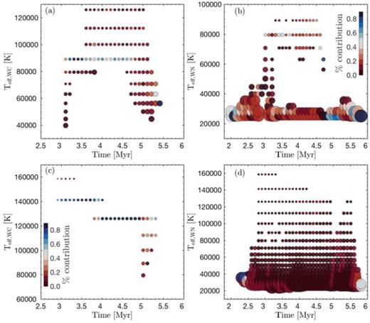
The selection of WR spectra as a function of time for Geneva high mass-loss (a)–(b) and Parsec (c)–(d) stellar evolutionary models assuming an IMF with a high mass cut off of 120 M⊙. At a given time, Teff and surface abundances of Hydrogen, Carbon, Nitrogen, and Oxygen of the isochrones are used to determine the WR subtype, then Teff and Rt are used to choose the spectrum from the PoWR grids. Left-hand panel: the selection of the WC spectra as a function of time and Teff (of the WR star), colour-coded to show the percentage of WC spectra of a given Teff (WR) which are chosen at a given time. Right-hand panel: the same as the left-hand panel, but for WN. The marker size denote the relative Rt, demonstrating that the spectra of WC subtypes chosen have Rt smaller than that of WN. Note that the spectral features between spectra of a given WR subtype can vary significantly depending on the Rt chosen.
The overall impact of the Geneva versus Parsec selection is illustrated in Fig. 2, which shows the evolutionary predictions for two prominent WR features; the blue (4550 ≲ λ [Å] ≲ 4750, left-hand panels) and red (5550 ≲ λ [Å] ≲ 6000, right panels) WR bumps, shown by the same colours in the figure. In panels (a)–(c) and (g)–(i), we show the evolution of the blue WR feature as predicted by the combinations of the Geneva high-mass-loss isochrones and PoWR, and Parsec and PoWR libraries, respectively, for sub-solar, solar and super-solar stellar metallicities. The variations in the shape of the blue WR feature reflect the differences in WR spectra selected from the PoWR library based on the Geneva and Parsec evolutionary models of the different stellar metallicities considered.
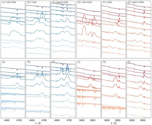
The evolution of the blue and red WR features as a function of stellar metallicity, log Zs/Z⊙ = –0.4 (sub-solar), 0.0 (solar), +0.3 (super-solar), for Geneva high mass-loss (a)–(f) and Parsec (g)–(l) isochrones. The time increases from the top to bottom panels from 1 to 5.5 Myr, in intervals of 0.5 Myr. The range in y-axes is the same for all the blue (and red) sets, and the assumed IMF upper mass cut is 120 M⊙.
As evident in Fig. 2, the blue WR feature tend to appear either as two emission peaks or as a single bump. If there are two peaks at approximately 4650 and 4686 Å, then the bluer of the two is typically attributed to the presence WC subtypes, though there can be some contribution from the late-type WN stars. A narrow blue peak indicates the presence of late-type WC stars, while early-type WC stars produce a broad emission peak, which may even extend and dominate over the redder component of the blue WR feature. The redder emission peak of the blue WR feature is attributed to WN subtypes. A broad redder component signals the presence of early-type WN stars, while a single or two narrow peaks indicates the presence of late-type WN stars (Crowther 2007; Sander et al. 2012; Todt et al. 2015).
Similarly, in panels (d)–(f) and (g)–(l) of Fig. 2, we show the evolution of the red WR feature, which is a signature of WC stars. The red WR feature consists of three peaks (clearly evident in panel d). The bluer of the three is a strong indicator of the presence of late-type WC stars, while the second is associated with early-type WC stars. The third, and the relatively weaker of the three, only appear as a separate peak if the star-forming region has a high number of late-type WC stars. Otherwise, it is usually blended with the second peak (Crowther 2007). So the presence of the red WR feature as three peaks in specific Geneva SSPs and lack thereof altogether in Parsec SSPs points to Geneva isochrones predicting a higher number of WC, particularly late-type WC, stars than Parsec. Note also that Fig. 1(a) shows that the Geneva isochrones sample the Teff, Rt, and age grid of WC stars more broadly than the Parsec isochrones.
The appearance and duration of the WR features are stellar metallicity dependent. With increasing stellar metallicity, the WR phase progressively extends in duration, the blue and red WR features start to appear at earlier times, and the features become more prominent. The Parsec SSPs, in particular, show this behaviour clearly. For instance, the average intensity of the blue (red) WR bump is enhanced by ∼2 (1.36) from sub-solar to solar metallicity over the age of 3−4 Myr, whereas it is diminished by ∼0.94 (0.6) between solar and super-solar metallicities. The slight decrease in strength of the WR features apparent in the super-solar metallicity SSPs, especially the blue component of the blue WR bump, is likely a result of the decrease in effective stellar temperatures with increasing metallicity, limiting the number of stars achieving the Teff threshold needed to become a WC star. Also, recall that we assume the Galactic (i.e. solar) metallicity for WR stars in the computation of the super-solar SSPs, which likely introduce some uncertainty to the shape and intensity of these features. In Geneva SSPs, however, these trends are evident to a lesser degree, likely as a result of the high mass-loss rates of the Geneva isochrones leading to the selection of a large number of late-type WC spectra. Nevertheless, the WR features (in both Geneva and Parsec SSPs) show an overall behaviour with stellar metallicity that qualitatively agrees with the spectroscopic observations of star-forming regions in nearby galaxies (Crowther 2007; Neugent & Massey 2019).
In the single-star stellar evolutionary predictions of Parsec and Geneva, the WR phase is short-lived, with the WR features rapidly changing in shape and intensity on time-scales smaller than 0.5 Myr. In contrast, the SSPs that take into account stellar rotational mixing and binary stellar evolution tend to show slower evolution in WR features, with the WR phase extended over a longer time-scale. For example, the bpass SSPs show the presence of WR stars until ∼100 Myr (Eldridge et al. 2017). While the effects of binary stellar evolution can be significant at low metallicities, at solar-like metallicities, however, these effects appear to be small enough such that single-stellar model predictions are adequate (Brinchmann, Kunth & Durret 2008a).
In Fig. 3, we compare the SSPs produced using the Geneva HML+CMFGEN, Geneva HML+PoWR, and Parsec + PoWR combinations over three different wavelength windows centred around prominent spectral features. As a result of the low-resolution of CMFGEN spectra (Hillier & Miller 1998), the Geneva HML+CMFGEN combination is unable to distinguish different peaks associated with the blue and red WR features, whereas both Geneva HML + PoWR and Parsec + PoWR allow the peaks to be resolved. It is also worth noting the nature of the evolution of the Balmer stellar absorption features – there is a WR feature centred around the Hα wavelength over some of the young ages considered in the figure, effectively decreasing the absorption equivalent width (EW) of Hα relative to Hβ.
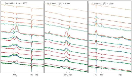
The evolution of simple stellar populations of solar stellar metallicity as predicted by Munari stellar library/Geneva isochrones/CMFGEN WR library (in blue), Munari stellar library/Geneva isochrones/PoWR WR library (in green), and Munari stellar library/Parsec isochrones/PoWR WR library (in red) combinations. The time runs from 1–5 Myr (top to bottom panels) in intervals of 0.5 Myr. The rest-frame wavelengths of He i from the left- to the right-hand panels are 4921.9, 5875.5, 6678.3, and 7065.7 Å, and the assumed IMF upper mass cut is 120 M⊙.
Finally, we have made some modifications to the PoWR library in order to produce WR features that are comparable with observations to date. We detail these modifications and their impact on the generated stellar templates in Appendix A. Briefly, we remove four spectra, two each, from the PoWR Galactic and LMC WC libraries, respectively, in order to reduce the significant enhancement of the blue component of the red WR bump evident in Fig. A1. This is a feature that has not been observed in the spectra of starbursting regions.
2.3.2 Chemical abundance dependance of the ionizing continuum
The chemical abundance dependence of the ionizing continuum predicted by the Geneva and Parsec isochrones is shown in Fig. 4.
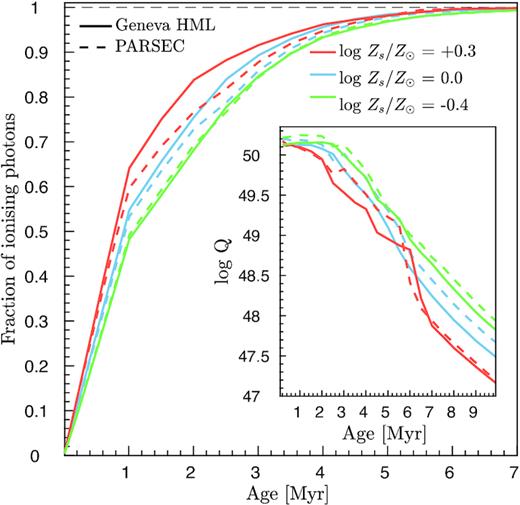
Chemical abundance dependence of the ionizing continua predicted by Geneva HML versus Parsec isochrones. The cumulative fraction of ionizing photons as a function of time and stellar metallicity (main panel), demonstrating that all the ionizing photons have essentially been emitted by approximately 6 Myr. The evolution of the ionizing photons (log Q) as a function of time for the same three metallicity for a starburst of 3000 M⊙ is shown within the inset. The zig-zag pattern, most notable in the super-solar models, highlight the short period over which the effects of the WR stars are prominent. Note that the qualitative trends in the evolution of log Q with metallicity are not affected by the assumed strength of the starburst, provided that the IMF is fully sampled. Increasing or decreasing the strength of the starburst, in this case, will systematically shift the evolutionary tracks upwards or downwards in log Q axis, respectively.
The number of ionizing photons emitted is a strong function of time, and within approximately 6 Myr virtually all ionizing photons have been emitted. At a fixed age, the cumulative fraction of ionizing photons emitted also show a clear dependence on stellar metallicity; the fraction of ionizing photons produced increases with increasing metallicity. Between Geneva HML and Parsec isochrones, the Geneva models lead to the production of a higher fraction of ionizing photons at a fixed age and metallicity, a result of their high mass-loss rates. Within the inset of Fig. 4, we show the evolution of log Q as a function of metallicity. On average, the higher metallicity models lead to a lower number of ionizing photons than lower metallicity counterparts, and between the Geneva HML and Parsec, the Parsec models produce relatively more photons than the Geneva HML. The zig-zag patterns evident in the log Q evolution, most notable in the super-solar metallicity models, correspond to the ages where the effects of the WR stars are heightened, wherein Parsec models occur at an earlier age.
2.4 The nebular model
We construct the nebular models self-consistently with cloudy (Ferland et al. 2013) using our modified starburst99 models, with different ages and stellar metallicities, as input. For the chemical composition of the gas, we adopt the solar-scaled abundances, except for Nitrogen, and H/He relation provided in Dopita et al. (2000). Nitrogen is assumed to be a secondary nucleosynthesis element above metallicities of 0.23 solar. Therefore, to scale Nitrogen with metallicity, we adopt the piecewise empirical relation, again, from Dopita et al. (2000). The assumption of a solar-scaled composition for the Antennae H ii regions is found to be reasonable by Lardo et al. (2015). Note also that the abundance of the stellar library incorporated into starburst99 is [α/Fe] = 0.0 (Table 1). So we have consistently used the same abundance pattern for the construction of the stellar and nebular components for the models of the H ii regions.
For the construction of the models for H ii regions, we assume a simple spherical approximation. While this is not strictly true, for regions dominated young, massive stars and their birth clouds, Efstathiou, Rowan-Robinson & Siebenmorgen (2000) and Siebenmorgen & Krügel (2007), for example, find a simple spherical approximation to be reasonable. Moreover, in the application of model library to the observed spectra (described in Section 3), we rely on emission-line intensity ratios rather absolute luminosities to minimize the effects of the assumption of spherical geometry.
2.4.1 Control of the ionization parameter
The strength of a starburst determines QH, and for each SSP, we consider cloudy models for different nH in the 10 ≤ nH[cm−3] ≤ 1000 and gas metallicity (Zg) in the −1.0 ≤ log Zg/Z⊙ ≤ +0.5 ranges assuming a spherical ionized region of fixed R (=3 pc). Following equation (2), we quantify the evolution of a starburst of given nH in terms of U, which is restricted to the −4.5 ≤ log U ≤ −0.5 range.5 For fixed R, the restricted range in U places constraints on the range in starbursts that can be probed (see also Table 2).
Even though we assume a fixed radius to generate the models, the radius can be varied a posteriori, allowing starbursts of any magnitude that generate ionization conditions in the U range considered to be probed. For example, below, we discuss the evolution of a number of quintessential nebular line ratios under different metallicity and density conditions, and a fully sampled IMF for starbursts of 3000, 6000, and 10 000 M⊙ for the radius defined in equation (2). The same ionization conditions, thus evolutionary predictions, are produced by starbursts of ∼8.3 × 10⁵, 1.6 × 10⁶, and 2.7 × 10⁶ M⊙ in an H ii region of radius ∼50 pc, the average for the H ii regions in the Antennae. It is this malleability of the models that we exploit in estimating physical properties of H ii regions in the second part of the paper.
The evolution of different nebular line ratios for a starburst of 3000 M⊙ is shown in Fig. 5. The diagnostics that have been most commonly used to classify the nature of a nebular excitation are [O iii]λ5007/Hβ, [N ii]λ6584/Hα, [S ii]λλ6717,31/Hα (Veilleux & Osterbrock 1987), as well as line intensity ratios based on [S iii]λ6312/[S iii]λ9069, [N ii]λ5755/[N ii]λ6548,84, etc. Those that use nebular lines that are close together in wavelength are generally preferred as they allow uncertainties related to reddening corrections to be minimized. For a fixed starburst, the diagnostics based on higher ionization species (e.g. [O iii]|$\rm {\lambda }$|5007/Hβ) show a swifter decline with time than their lower ionization counterparts. For a fixed age, the U of higher metallicity models is lower than that of lower metallicities, and likewise, the predicted ratios. The zig-zag pattern visible in the evolutionary tracks, particularly prominent in super-solar metallicity models, is caused by the brief hardening of the stellar radiation field resulting from the appearance of the WR stars. The ageing tracks with low-to-high nH show a low-to-high variation in line ratios, except the [O iii]|$\rm {\lambda }$|5007/Hβ track that shows the opposite trend for ages ≳5 [Myr]. Note, however, that the predicted [O iii]|$\rm {\lambda }$|5007/Hβ for old ages is too faint to be detected observationally.
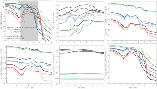
The evolution of different line luminosity ratios as a function of nH and metallicity for a burst of star formation of strength 3000 M⊙ for a model H ii region of a fixed radius. The gas and stellar metallicities are approximately similar. The log U (a function of the burst strength, nH, metallicity, and time) corresponding to different times (for nH = 100 cm−3) is indicated along the sub- (green) and super-solar (red) tracks. The shading in panel (a) denote the approximate (overall across all three metallicities considered, the individual cases show small variations duration of the WR phase) duration of the WR phase.
The evolutionary predictions in the BPT (Baldwin, Phillips & Terlevich 1981) plane under different metallicity and nH conditions is shown in the top panel of Fig. 6. The black solid and dashed lines denote the Kewley et al. (2001) and Kauffmann et al. (2003) demarcations separating active galactic nuclei from H ii regions, with the grey-dashed line indicating the excitation sequence determined by Brinchmann et al. (2008b) from a sample of nearby star-forming galaxies. For each track, the age increases approximately diagonally from 0.5 Myr (upper left-hand panel) to Tlast, with Tlast being the age of the last point visible in the parameter space of the figure.
![Top panel: BPT diagnostics from cloudy modelling of a starburst of 3000 M⊙. The line ratios evolve in the direction shown by the black ’age’ arrow. The different colours correspond to different metallicities, while different shadings, from dark-to-light, of the same colour, denote nH = 1000, 100, and 10 cm−3, respectively. The legend shows the last age of the data point of a given (Z, nH) still visible in the parameter space shown before moving off the diagram. The vectors show the effect of doubling the burst strength (i.e. from 3000 to 6000 M⊙). The black dashed and solid lines show the Kewley et al. (2001) and Kauffmann et al. (2003) demarcations, respectively, and the dashed grey line denotes the fit to the SDSS data from Brinchmann et al. (2008b). Bottom panel: The difference in [O iii] $\rm {\lambda }$5007/Hβ and [N ii] $\rm {\lambda }$6584/Hα between the 3000 and 6000 M⊙ starburst as a function of time. The colours are the same as in the top panel, and in addition, the solid, dashed, and dotted lines correspond to nH = 1000, 100, and 10 cm−3, respectively. Note that even though at earlier ages the nH = 1000 cm−3 tracks appear to show a progressively larger enhancement in [O iii] $\rm {\lambda }$5007/Hβ with increasing metallicity, at a fixed [O iii] $\rm {\lambda }$5007/Hβ, the [O iii] $\rm {\lambda }$5007/Hβ increases with decreasing metallicity as expected given the Te dependence on metallicity. Note that the burst strengths explored here are for model H ii regions of a fixed radius.](https://oup.silverchair-cdn.com/oup/backfile/Content_public/Journal/mnras/497/3/10.1093_mnras_staa2158/1/m_staa2158fig6.jpeg?Expires=1716411860&Signature=UbfC9EgBDLQQglqYj5F7yAjDRHGDGshexDFNwook7-2vadzOjXKUW~gxgBCrauqLQRruzYH6IXLULpuj3gRzzd5w55blUeIMCQsJrbCw1ZNj6q1~yprdp5ABW4sj~T3RqJE3aPmE9cLB2FCVwVgq5rDaMkkJWoxPpEnatWYq6ohLwQFZNFQw3ekW0X6Rm5kfZBO-8oSo6jc5~GHdkbIJvWD4l-Xio72qi1UU43Bh3gheJdWGXnozfsYjh3NKdTuHhdQfAlXfAJf7FlqtVSJZFTJfF9Im1BdoVOfkZDXHYPocIzEfygioJBbASFigS7Y8ei3fABtRhNiSucxyyjfXNg__&Key-Pair-Id=APKAIE5G5CRDK6RD3PGA)
Top panel: BPT diagnostics from cloudy modelling of a starburst of 3000 M⊙. The line ratios evolve in the direction shown by the black ’age’ arrow. The different colours correspond to different metallicities, while different shadings, from dark-to-light, of the same colour, denote nH = 1000, 100, and 10 cm−3, respectively. The legend shows the last age of the data point of a given (Z, nH) still visible in the parameter space shown before moving off the diagram. The vectors show the effect of doubling the burst strength (i.e. from 3000 to 6000 M⊙). The black dashed and solid lines show the Kewley et al. (2001) and Kauffmann et al. (2003) demarcations, respectively, and the dashed grey line denotes the fit to the SDSS data from Brinchmann et al. (2008b). Bottom panel: The difference in [O iii] |$\rm {\lambda }$|5007/Hβ and [N ii] |$\rm {\lambda }$|6584/Hα between the 3000 and 6000 M⊙ starburst as a function of time. The colours are the same as in the top panel, and in addition, the solid, dashed, and dotted lines correspond to nH = 1000, 100, and 10 cm−3, respectively. Note that even though at earlier ages the nH = 1000 cm−3 tracks appear to show a progressively larger enhancement in [O iii] |$\rm {\lambda }$|5007/Hβ with increasing metallicity, at a fixed [O iii] |$\rm {\lambda }$|5007/Hβ, the [O iii] |$\rm {\lambda }$|5007/Hβ increases with decreasing metallicity as expected given the Te dependence on metallicity. Note that the burst strengths explored here are for model H ii regions of a fixed radius.
The effect of raising nH is to enhance both the [O iii] |$\rm {\lambda }$|5007/Hβ and [N ii] |$\rm {\lambda }$|6584/Hα due to the increased rate of collisional excitation. At a fixed nH, the decline in log U with increasing metallicity pushes the BPT predictions towards lower [O iii] |$\rm {\lambda }$|5007/Hβ and higher [N ii] |$\rm {\lambda }$|6584/Hα values. The low (high) metallicity and low (high) nH predictions form the left (right) edge of the sequence, suggesting that it is unlikely to observe a low metallicity H ii region with a low U value.
The vectors shown in Fig. 6 highlight the effect of doubling the strength of the starburst with each vector indicating the magnitude and the direction of the movement of a given point. As a consequence of the increase in log U, the effect in large is to enhance the [O iii] |$\rm {\lambda }$|5007/Hβ and decrease the [N ii] |$\rm {\lambda }$|6584/Hα. At high metallicities, however, the [O iii] |$\rm {\lambda }$|5007/Hβ corresponding to nH = 100 and 10 cm−3 show a decrease with increasing log U. This is further illustrated in the bottom panel of Fig. 6, where we quantify the change in [O iii] |$\rm {\lambda }$|5007/Hβ and [N ii] |$\rm {\lambda }$|6584/Hα from 3000 to 6000 M⊙ as a function of time. This behaviour of [O iii] |$\rm {\lambda }$|5007/Hβ and [N ii] |$\rm {\lambda }$|6584/Hα can be explained by the relationship between log U, electron temperature (Te), metallicity and nH.
In Fig. 7, we show the cloudy predictions of the volume-averaged Te dependence on metallicity and log U for nH = 10, 100, 1000 cm−3, assuming that the metallicity of stars is similar to that of the star-forming gas from which they were formed. At a fixed metallicity, Te varies relatively weakly with both log U and nH, whereas, at a fixed log U and nH, Te shows a significant dependence on metallicity. On average, Te increases with increasing log U at low metallicities and decreases with increasing log U at high metallicities. Te also increases with increasing nH at all metallicities, relatively more steeply at high metallicities than at low metallicities. In comparison to the Te dependence on metallicity, however, its dependence on nH is relatively weak.
![The dependence of the volume-averaged Te on metallicity and log U for nH = 10, 100, 1000 [cm−3] for a stellar population of aged 3 Myr. The contours denote constant Te values.](https://oup.silverchair-cdn.com/oup/backfile/Content_public/Journal/mnras/497/3/10.1093_mnras_staa2158/1/m_staa2158fig7.jpeg?Expires=1716411860&Signature=WRgMw8dH~JAn6gEq8FImpN29qeATLvBbiztYoOOLDgQaRxXxAdV6oYAk1OgdZwiCJ-4dorWzZcIMtdHAGEa72JmhkeNUHFs8ZaUUGmx8G3CP~GKSV7g1dAvwQwA7nKbNGHN6R9FMxZhTCd6vYUsldMhLu1yOALrfPdH5TltgrmtYR~2vPTySAzjb-ZnqbUQ6QqirwJ6ihM9XCpt2dLDTsNILfQfPKZOglQK4mluAWOtCRIwJwngNVaavPxKk-Z1ZthwMPd5rM1jrkZTr7q~Oxh-nGTcliSll~6dHcmF75zLvk7kMqkEowruGbLyZXm0dshyPxpd2LVdqPbq~OJnodg__&Key-Pair-Id=APKAIE5G5CRDK6RD3PGA)
The dependence of the volume-averaged Te on metallicity and log U for nH = 10, 100, 1000 [cm−3] for a stellar population of aged 3 Myr. The contours denote constant Te values.
The Te-metallicity-log U relationship is primarily driven by the cooling efficiency in an H ii region, which is largely a function of gas metallicity. At very low log Zg/Z⊙ (e.g. ≲−1), the contribution of collisionaly excited metal lines to cooling is negligible, thusTe largely increases as a function of log U. At high log Zg/Z⊙, however, the cooling efficiency increases as a function of log U, resulting in a decrease in Te as a function of increasing log U. As the cooling efficiency is, on average, an inverse function of density6 (nH), Te increases with increasing gas density (Ferland 1999; Byler et al. 2017).
As such, Te does not always increase as a function of log U. This means that even though doubling the strength of a starburst increases log U, it leads to a decrease in Te at high metallicities. At nH of 100 cm−3, in particular, an increase in log U corresponds to a larger decline in Te (i.e. the constant Te contours are closer together at high metallicities than at low metallicities, Fig. 7 middle panel). Given the sensitivity of [O iii] to Te, the decline in Te with increasing log U (at high metallicities) and nH = 100 cm−3 leads to a decrement in [O iii] |$\rm {\lambda }$|5007/Hβ. The decline in Te with increasing log U is still high enough at nH = 10 cm−3 to cause a decrease in [O iii] |$\rm {\lambda }$|5007/Hβ, albeit smaller in comparison to nH = 100 cm−3 (Fig. 6 bottom panel). At nH = 1000 cm−3, the difference in Te caused by doubling the burst strength is sufficiently small as the Te contours are spanned out (Fig. 7 right-hand panel), resulting in an enhancement in [O iii] |$\rm {\lambda }$|5007/Hβ with increasing log U as expected.
2.4.2 The importance of the nebular continuum
The continuous emission spectrum produced by the ionized gas can contribute significantly to the observed spectrum. The total nebular continuum is dominated by the emission from the free–bound recombination processes of hydrogen and helium ions and electrons, free–free (Bremsstrahlung) transitions in the Coulomb fields of H+, He+, and He2+ and two-photon (bound-bound) decay of the 22S1/2 level of H i and He ii, and 21S0 level of HeI, which is relatively less important (Ercolano & Storey 2006).
The free–bound continuum shows discrete jumps due to the discrete nature of the lower energy levels at the ionization energy, followed by continuous emission to higher energies. It is also a dominant contributor to the total nebular continuum over optical wavelengths, and, as a product of radiative recombination processes, its absolute intensity depends strongly on the ionization parameter, with the shape only showing a small dependence (Fig. 8a). The free–free continuum is power law like (∝ν−2) in shape and progressively becomes a dominant contributor to the total nebular continuum towards the infrared wavelengths. The total energy radiated increases as the electron temperature (Te) is raised.
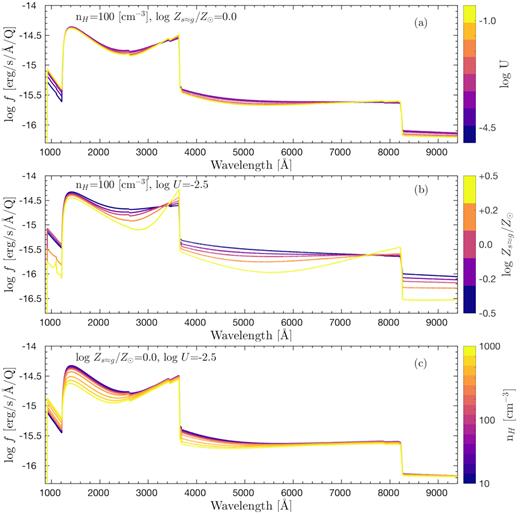
The behaviour of the nebular continuum of a stellar population aged 3 Myr with respect to three different properties. (a) The nebular continuum as a function of the ionization parameter (U) at nH = 100 cm−3 and log Zs ≈ g/Z⊙ of 0.0 (s ≈ g means that the stellar metallicity is assumed to be the same as the gas metallicity). While the shape of the nebular continuum shows a little dependence on log U, the absolute normalization depends strongly on the number ionizing photons (QH). Since we show the nebular continuum in the unit of erg s−1 Å−1 Q−1, the absolute normalization dependence on the number of ionizing photons has been removed. (b) The nebular continuum as a function of log Zs ≈ g/Z⊙ at nH = 100 cm−3 and log U = –2.5. The shape of the nebular continuum is primarily informed by the free–bound and free–free continua dependence on Te. (c) The nebular continuum as a function of nH at log Zs ≈ g/Z⊙ of solar and log U = –2.5. The effects of nH is largely confined to the bluer wavelengths, highlighting the dependence of the 2γ continuum on nH.
The dependence of the nebular continuum on metallicity, again highlighting the underlying dependence on Te, is shown in Fig. 8(b). The lower metallicity models (higher Te) show higher continuum emission, and lower magnitudes for discontinuities at 3646 and 8207Å than the higher metallicity models. The free–bound continuum contribution to the total nebular continuum dominates at higher metallicities (lower Te), producing a total continuum with more pronounced saw-tooth like jumps at 3646 Å and 8207 Å. With increasing Te, the free–free continuum becomes progressively more significant, and the power law like free–free continuum starts to dilute the saw-tooth structure of the free–bound continuum. As the relative contribution of the free–free contribution at infrared wavelengths is higher than at bluer wavelengths, the amplitudes of the recombination edges at longer wavelengths will be more affected.
The two-photon (or 2γ) continuum is a result of the radiative decay from the 22S to12S level of hydrogenic species (H i and He ii). A radiative decay to the 12S level is strongly forbidden, however, a transition can take place if two photons with sum of energies equal to that of Lyα is emitted. The decay of 21S level of He i also produces, albeit a weaker, two-photon continuum (Nussbaumer & Schmutz 1984; Drake 1986; Draine 2011). Hence the 2γ continuum has a peak at half the Lyα frequency and a natural cut-off at the Lyα frequency, highlighting the importance of the 2γ continuum for near-, and far-ultraviolet observations.
The density of the plasma can have a significant impact on the 2γ continuum. As the radiative lifetime of the 22S level is long, the 22S level can be de-populated through angular momentum changing collisions (22S → 22P) with other ions and electrons before a two-photon decay can occur. The radiative decay to 12S level from 22P level may then occur by emitting a Lyα photon. Therefore, while at low densities, the 2γ continuum dominates the free–bound continuum, it can be suppressed in H ii regions with high densities (∼105 cm−3) (Aller 1984). The dependence of the 2γ continuum on nH is shown in Fig. 8(c). The ‘bump’ at ∼1500 Å is primarily caused by the 2γ continuum, with lower nH models showing higher continuum emission over the UV wavelength regime than their higher density counterparts.
In young star-forming regions, the nebular continuum can dominate the total continuum, especially around the wavelengths of the Balmer and Paschen discontinuities. The ratio of the nebular to total (nebular + stellar) continuum with respect to different metallicities for stellar populations of 1, 3, and 5 Myr age is shown in Fig. 9. For stellar populations of ages between 1 and 4 Myr, the nebular continuum contributes between 20 and 80 per cent of the emission.
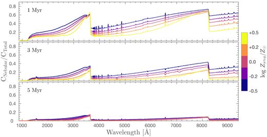
The ratio of the nebular continuum to total (stellar + nebular) continuum as a function of metallicity for fixed log U of –2.5 and nH of 100 cm−3, and for SSPs of aged 3 and 5 Myr. Five different metallicities are considered, where the metallicity of stars is assumed to be similar to that of gas from which they are formed.
3 SELF-CONSISTENT MODELLING OF STELLAR AND NEBULAR FEATURES
Here, we focus on the development of the model libraries (Section 3.1) and the model fitting procedures (Sections 3.2–3.4).
In the construction and the fitting of the model libraries below, we treat stellar and gas metallicities as independent parameters. The reason being that the starburst data set used in this study (Section 4) has high enough continuum signal-to-noise ratio, with spectra showing prominent features originating from massive stars, that we can constrain the stellar metallicity independently of the gas metallicity. In the absence of high-quality data, however, it is acceptable to approximate the stellar metallicity to that of gas or use the gas metallicity as a prior in constraining that of stars, as stellar metallicity might be expected not to differ significantly from that of the surrounding star-forming gas.
3.1 The stellar and nebular model library
We construct two separate model libraries using the Geneva and Parsec isochrones. Each library is parametrised by stellar metallicity (Zs), gas metallicity (Zg), age, nH, and strength of the starburst, with the Kroupa IMF high-mass cut-off assumed to be fixed. We describe the ranges and the sampling of each parameter in detail in Table 2.
The model continua of young stellar populations show a substantial evolution. Over the <5 Myr time-scale, the nebular continuum contribution to the total can be significant (Fig. 9), with the nebular continuum being largely featureless except for the jumps. With increasing age, the nebular continuum contribution to the total continuum diminishes while more prominent continuum structures, e.g. TiO bands around 7000Å, and various absorption features appear.
The behaviour of the model emission-line ratio diagnostics is shown in Fig. 10. The colour-coding is the same as in Fig. 5, the thick-to-thin lines denote high-to-low nH, and the dotted versus solid lines of the same colour and thickness correspond to starbursts of 100 M⊙ and 10 000 M⊙, respectively. The black and red arrows denote the direction of the increase in age of the stellar population along each model track and dust vectors, respectively. The underlying data points denote the distributions of the observed emission-line ratios of the H ii regions in the Antennae galaxy from Weilbacher et al. (2018), with the cross to the left indicating the average errors associated with the observed fluxes.
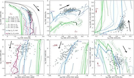
The behaviour of predicted nebular lines in different diagnostic diagrams. The different colours correspond to different metallicities, while the line thickness and styles denote the nH values and burst strengths, respectively. The ages increase along each track with the black arrows pointing to the general direction of increase. The filled black circles on thick-solid lines denote age steps in 0.5 Myr, starting from an age of 1 Myr. If the 1 Myr age point is outside the parameters space of the diagram, we show the youngest age within the parameters space next to the corresponding symbol. The red arrows denote the dust vectors computed assuming one-magnitude extinction in Hα and the Calzetti (2001) extinction law. The zig-zag patterns evident are a result of the appearance of WR stars. For clarity, we have only shown the super-solar metallicity predictions for the two left-most diagnostics diagrams. The crosses indicate the distribution of the H ii regions in the Antennae galaxy. A signal-to-noise cut is applied to the observations based on the signal-to-noise ratio of the weakest line in a given set of emission line ratio diagnostics. As noted in Section 3, the stellar and gas metallicities are independent parameters of the model libraries, however, here we make the approximation that Zs ≈ Zg for clarity. Also, the burst strengths (|$\mathcal {B}$|) explored here are for model H ii regions of the fixed radius defined in equation (2).
The most substantial changes evident in the model evolutionary tracks appear to be driven by metallicity. In the BPT plane (top left-hand panel), the sub-solar Z tracks are closer together than other metallicity models such that an increase in burst strength affect [O iii]/Hβ, a diagnostic sensitive to both U and the age of the stellar population, more significantly than [N ii]/Hα, a diagnostic sensitive to abundance. Note, however, that this assertion is largely true for later ages, as the changes in both [O iii]/Hβ and N ii]/Hα appear to be significant and somewhat similar at earlier ages. In contrast, [N ii]/Hα show a greater change than [O iii]/Hβ with increasing metallicity.
The behaviour of [O iii]/Hβ in low metallicity models can largely be explained by Te (see also Section 2.4.1). As shown in Fig. 4, at a given burst and age, the central stars of low-metallicity H ii regions have higher effective temperatures, thus higher U than high-metallicity regions (top left-hand panel of Fig. 5). Therefore, in these regions, which are already characterized by higher excitation species than high-metallicity regions, an enhanced burst will further act to amplify the degree of excitation of [O ii]. Furthermore, Nitrogen has a substantial secondary nucleosynthesis contribution over a large range in metallicity, except at very low metallicities, (Matteucci 1986; Dopita et al. 2000) such that the abundance ratio of a secondary to a primary element, e.g. N/O, will systematically increase with nebular abundance. Therefore, the lack of a change in [N ii]/Hα in low-metallicity models is likely due to low N+ abundances.
In high-metallicity H ii regions, which are characterized by low Te, the higher excitation energy transitions (e.g. O+ to O++) are suppressed, while the relatively lower energy species (e.g. N++) are continuously excited (Dopita et al. 2006). This process along with the relatively high Nitrogen abundances likely drive the increase in enhancement (decrement) evident in [N ii]/Hα ([O iii]/Hβ). In fact, it is this sensitivity of [N ii] to abundance that makes the [N ii] λ6584/Hα a useful abundance diagnostic.
Similarly, the observed trend of [Ar iii] λ7135/[O iii] λ5007 with respect to [N ii] λ6584/Hα (top right-hand panel) for a large part is due to the inverse relationship between metallicity and Te, which translates into an increase of the [Ar iii] λ7135 and [O iii] λ5007 emissivity ratios. According to Stasińska (2006), the decrease in U with increasing metallicity also adds to the observed trend in [Ar iii] λ7135/[O iii] λ5007, however, it does not play a dominant role.
The [O iii], [N ii] and [S iii] have high-energy structures with considerably different excitation energies, such that the ratio between the lines originating from different excitation energy levels can be utilized as temperature diagnostics (Osterbrock & Ferland 2006; Peimbert et al. 2017). So in Fig. 10 bottom left-hand panel, we show the model predictions7 for the ratio of [S iii] λ6312Å, which originates from the excitation energy of level 1S0 with 3.37 eV, to [S iii] λ9069, the line resulting from the lower excitation level of 1D with 1.4 eV. Similarly, in the bottom middle panel of Fig. 10, we show the ratio of [N ii] λ5755Å, corresponding to the excitation energy of the level 1S0 with 4.05 eV, to [N ii] λ6584Å, corresponding to the excitation energy of the level 1D of 1.9 eV (Luridiana, Morisset & Shaw 2015). Overall, the model evolutionary tracks show a large spread both as a function of metallicity, emphasising their underlying sensitivity to Te, and nH.
Finally, as is evident in Fig. 10, a single diagnostic alone cannot accurately trace an entire H ii region, which is a complex ionization/thermal structure. The high ionization lines (e.g. [O iii], [Ar iii], [S iii]) are strongly sensitive to the ionization parameter, which itself depends on the age. Therefore, these species will be mostly produced in very young H ii regions and, with increasing age, will be limited to tracing the innermost of the H ii regions (Byler et al. 2017). Consequently, the Te estimated from high ionization line based diagnostics like [O iii] and [S iii], and nH measured from [Cl iii] and [Ar iv] will only be representative of the innermost regions of a H ii region. In contrast, the [N ii], [O ii], and [S ii] lines are stronger in the outer parts of an H ii region, where the ionization is low. In modelling integrated spectra of star-forming galaxies, the lower ionization species will also get a much greater weighting from the aged H ii regions than the higher excitation species like O++. The temperature and density diagnostics based on these species, likewise, mostly trace the outermost of H ii regions. In concluding this section, it is worthwhile to note that the model line ratio diagnostics sample the parameter space of the observed emission-line ratios, suggesting that our model libraries are capable of (approximately) reproducing the observations.
3.2 Fitting for the stellar and nebular continua
Our model fitting routines are built on platefit, a code originally written to perform a non-negative least-squares fit with dust attenuation modelled as a free parameter to find the best-fitting stellar continuum model for a given spectrum (Brinchmann et al. 2004; Tremonti et al. 2004). In this study, we update and equip platefit with additional routines to allow self-consistent modelling of stellar and nebular continua, and nebular emission-line ratios using the libraries described in Table 2.
For the continuum fitting, the dust attenuation is modelled as a free parameter using a simple attenuation curve, τ(λ) ∝ λ−1.3. The exponent of −1.3 is recommended by Charlot & Fall (2000), which was observed to correspond to the middle range of the optical properties of dust grains between the Milky Way, the LMC and the SMC, and was found to be appropriate for modelling the attenuation of birth clouds by da Cunha, Charlot & Elbaz (2008). We have tested other common attenuation laws in the literature (e.g. Prevot et al. 1984; Calzetti et al. 2000), and their impact on the outcomes of the fitting appear to be minimal. In this analysis, we assume that the young and old stellar populations are attenuated to the same extent.
The SFHs of starbursting H ii regions are likely episodic than constant or exponential-like. Wilson & Matthews (1995), for example, find evidence for burst-like SFHs in local luminous H ii regions. Therefore, following the underlying assumption that the SFH can be approximated as a sum of discrete bursts, we use platefit to fit the underlying stellar and nebular continua of a given spectrum to extract the individual models most likely contributing to its SFH. The weights of the extracted models are defined relative to the luminosity at 5500 Å.
Strictly speaking, to preserve self-consistency, the stellar and nebular continua must be modelled as a function of all the parameters of the model library (Table 2). The model libraries described in Section 3.1 are comprehensive in both the range in parameters probed and the sampling of the parameter space. As such, the use of the full model library in the fitting can be computationally expensive. There are, however, specific model parameters that do not contribute to describing the shape of the stellar and nebular continua over the MUSE rest wavelength coverage of the Antennae spectra. These parameters, therefore, can be set to fiducial values without sacrificing self-consistency. For example, recall that the variations in nH affect mostly the 2γ continuum, whereas the shape of the nebular continuum over the 4600−9300 Å range only show a small dependence (see Fig. 8c). Similarly, the shape of the nebular continuum shows no dependence on U (see Fig. 8a), which we use to trace the strength of the starburst. Consequently, we can perform the platefit stellar and nebular continua fitting as a function of three model parameters (i.e t, Zg, Zs), instead of five, to extract the individual light-weighted underlying stellar populations likely contributing to the SFH as a function of Zg and Zs. The best-fitting velocity dispersion is determined from the continuum fitting, assuming trial velocity dispersions to converge to the solution that minimizes the chi-squared of the fit.
After subtracting the best-fitting stellar and nebular continuum (derived from adding the individual light-weighted stellar population models) in each Zg and Zs from the observed spectrum, we model all the emission lines with Gaussians simultaneously. We were able to model the majority of the Antennae spectra this way. A subset of spectra, however, required removing remaining residuals by fitting a Legendre polynomial of degree 15 before modelling the emission lines. The residuals, in most part, can be used to inform the improvements needed in population models, in attenuation models and fitting routines, as well as the issues related to data reduction. Ideally, the uncertainties from the continuum fitting should be folded-in to the emission-line flux errors without adjusting the best-fitting model. It is, however, difficult to ascertain the true uncertainties without duplicate observations of the Antennae galaxy. Encouragingly, the best-fitting models in each Zg and Zs show a good agreement with the data over the wavelength ranges of the strong emission lines (e.g. Hα, Hβ, [O iii] λ5007Å, [N ii] λ6548, 84Å, [S ii] λ6717, 31Å and redwards of the Paschen jump) without requiring a fit to the residuals. On the other hand, the weak nebular lines (e.g. [Cl iii] 5517,37Å, [O ii] 7323,32Å and weak He lines) are affected by any mismatch between the best-fitting models and the data, thus benefit from a fit to the residuals.
3.3 Fitting for the nebular emission-line intensity ratios
To match the nebular model predictions with the individual light-weighted underlying stellar populations extracted during the continuum fitting process, we weight the respective nebular model by the lightweight of the respective stellar population. The best-fitting nebular model is, then, given by the sum of individual light-weighted nebular models. Therefore all quantities extracted from the fitting process are light weighted. The nebular models exist only for the <10 Myr stellar populations, and we assume that these young populations are responsible for all observed nebular emission.
For the fitting, we adopt the Bayesian approach outlined in Brinchmann et al. (2004), Brinchmann et al. (2013) and derive the probability density functions (PDF) for the physical properties of interest. The overall fitting process is illustrated in Figs 11 and 12, where we show how the likelihood distributions of six different properties are constrained progressively with the addition of emission-line ratios. The columns, from the left- to the right-hand side, correspond to the strength of the burst in units of M⊙, nH in units of cm−3, gas (Zg) and stellar (Zs) metallicities in units of solar metallicity, e− temperature (Te) in unit of K, and the age of the <10 Myr stellar population (tyoung) in unit of Myr. The top row of panels shows the likelihood distributions after the continuum fitting process and with one emission-line ratio added. Already at this stage, the likelihoods of Zg, Zs, Te, and tyoung reflect the constraints imposed by the continuum fitting process, and as we do not fit for U and nH during the continuum fitting (Section 3.2), the burst strength and nH PDFs are not constrained at all. Between the first (i.e. top panel) and second row, we add another line ratio, and so on, until most of the properties of interest are strongly constrained. We consider a range of line ratios (e.g. see Fig. 10 for some examples), particularly those based on strong lines.
![The result of the fit to the Antennae H ii region A1439 using Parsec-based model library. Each column corresponds to the PDFs for one derived property as progressively more emission-line ratios are added. As the spectra used for this analysis contain a large number of emission lines, the $\hat{\rm {R}}_3$–$\hat{\rm {R}}_6$ show the PDFs obtained from using various different emission-line ratios and should be viewed as averages, while R1 and R2 are fixed to [O iii] λ5007Å/Hβ and [S ii] λ6717, 31Å, respectively. In most fits, $\hat{\rm {R}}_3$–$\hat{\rm {R}}_6$ represents a mixture of strong and weak lines. The columns from the left- to right-hand panel shows the strength of the burst, nH, gas and stellar metallicities with respect to solar, Te, and the age of the <10 Myr stellar population. Note that all these quantities are light weighted. The top row shows the PDFs after fitting the total continuum, which adds constraints on gas and stellar metallicities, Te and light-weighted age of the young stellar populations. The strength of the burst and nH are primarily constrained through nebular line luminosity ratios, therefore their PDFs essentially show the flat priors adopted.](https://oup.silverchair-cdn.com/oup/backfile/Content_public/Journal/mnras/497/3/10.1093_mnras_staa2158/1/m_staa2158fig11.jpeg?Expires=1716411860&Signature=t5Wb2gcGTKesqFNbCfAvFVkZki837QYaCZNHJHASJfsGtDqewPeTbLV84SDNcO0oEA8GvAYJw-eb~WcKDaCMWgPjE-iLV-BE3zWZw0wI2fJAfN4NHtZSMpHBnI0Sd7lDwt3t5gfq~7khQilmE07AL2qf3ioe7CvSmD~BU3rQEvcwUqa2vNP-IhRHb5K2foTd60azVh5wfdvFc-3TIVuiOGlVHeP3hDll6T3Q1gsneiiYzJiycrOmkYQakajT~HJfw~z9KBx67TWTgBSjFqTjxTmuJreLgNqMvHUve3TKpvo-npF-BYxMaD8PDX84m87PPb41-~JAKe3ZyYb-V9SWSQ__&Key-Pair-Id=APKAIE5G5CRDK6RD3PGA)
The result of the fit to the Antennae H ii region A1439 using Parsec-based model library. Each column corresponds to the PDFs for one derived property as progressively more emission-line ratios are added. As the spectra used for this analysis contain a large number of emission lines, the |$\hat{\rm {R}}_3$|–|$\hat{\rm {R}}_6$| show the PDFs obtained from using various different emission-line ratios and should be viewed as averages, while R1 and R2 are fixed to [O iii] λ5007Å/Hβ and [S ii] λ6717, 31Å, respectively. In most fits, |$\hat{\rm {R}}_3$|–|$\hat{\rm {R}}_6$| represents a mixture of strong and weak lines. The columns from the left- to right-hand panel shows the strength of the burst, nH, gas and stellar metallicities with respect to solar, Te, and the age of the <10 Myr stellar population. Note that all these quantities are light weighted. The top row shows the PDFs after fitting the total continuum, which adds constraints on gas and stellar metallicities, Te and light-weighted age of the young stellar populations. The strength of the burst and nH are primarily constrained through nebular line luminosity ratios, therefore their PDFs essentially show the flat priors adopted.
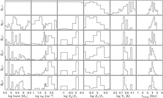
The PDFs shown in Figs 11 and 12 are derived from fitting the Parsec and Geneva libraries, respectively, to the Antennae H ii region, A1439. Except for the [S ii] λ6717, 31Å and the BPT diagnostics that correspond to R1 and R2, the rest (|$\hat{\rm {R}}_3$|–|$\hat{\rm {R}}_6$|) of the ratios include various strong and weak emission lines involving [O iii], [S iii], [Cl iii], [Ar iii], [S ii], [O ii], [N ii], and Balmer lines (see Fig. 10 for the behaviours of some of the line ratios considered with respect to models), and are included in the fits in no particular order. Note that as there are more than six different emission-line ratios available for the Antennae data, we run the final stage of the fitting process several times with different emission-line ratios for |$\hat{\rm {R}}_3$|–|$\hat{\rm {R}}_6$|, and consider combinations of low- and high-ionization line ratios to extract all potential metallicity, nH and age solutions. The |$\hat{\rm {R}}_3$|–|$\hat{\rm {R}}_6$| PDFs should, therefore, be viewed as averages.
The first column shows the PDF of the burst strength, which is somewhat poorly constrained. As discussed earlier, the presence of different ionization structures within an H ii region means that different ionization species dominate different regions. Given that we determine the burst strength that can produce observed emission-line ratios using U, with lower versus higher ionization lines pointing to low and high U values, the burst strength can indirectly be sensitive to the ionization structure of an H ii region. Consequently, the PDF of the burst strength can yield multiple solutions as shown.
The nH is shown in the second column. Immediately following the inclusion of the [S ii] λ6717, 31Å ratio (R2), a well-known gas density diagnostic, the PDF appear to converge. The [S ii] λ6717, 31Å is, however, a probe of the low-density, low-ionization zones of an H ii region, therefore, with the inclusion of additional line diagnostics, especially those with higher excitation energies, the PDF either converges to provide an average nH or two potential nH solutions. Note also that there is a degeneracy between nH and burst strength, where high nH imply low-ionization parameters, and hence, low burst strengths, and vice versa.
In the third column, we show the PDFs of the gas metallicity in units of solar metallicity. The continuum fitting, principally the Paschen jump, provides some constraints on Zg as evident in the first PDF. The strongest constraints, however, appear to come from the emission-line ratio diagnostics, which can be expected given the dependence of some emission lines (e.g. [N ii], [S ii]) on abundance.
The PDFs of the stellar metallicity are presented in the fourth column. As apparent in the first PDF, the continuum model fitting, informed in particular by the WR bumps and the Paschen jump, add strong constraints on Zs. The inclusion of the emission-line ratio diagnostics appears to strengthen the constraints on Zs further. Overall, we find that constraining Zs is generally more challenging than constraining Zg – see Section 3.4 for a discussion on the possible ways of improving the robustness of Zs derivations.
We show the likelihood distributions of the Te in the fifth column. Since Te is a strongly decreasing function of metallicity (Fig. 7), the continuum fitting process notably constrains the PDF. Recall that at solar-like metallicities, the Te dependence on the burst strength (i.e. U) is weak (see Fig. 7), therefore, the lack of strong constraints on the burst strength parameter does not significantly influence the PDFs of the Te and nH.
The final column shows the likelihood distribution for the age of the young (i.e. <10 Myr) stellar population. Owing mainly to the presence of WR features, the PDF of the young ages is tightly constrained by the continuum fitting process, with the relatively little constraint imposed by the emission-line ratio diagnostics.
The best-fitting spectral models corresponding to the final PDFs shown in Figs 11 and 12 are presented in in the top and bottom panels of Fig. 13, respectively. The best-fitting spectral model is shown green, the best-fitting model adjusted with a Legendre polynomial fit to the residuals in red and the observed spectrum in black. The inset within each panel shows the distribution of ages of the underlying stellar populations contributing to the best-fitting spectral model (i.e. the best-fitting SFH).
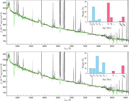
The best-fitting Parsec (top panel) and Geneva (bottom panel) models corresponding to the constrained PDFs of the Antennae H ii region A1439 shown in Figs 11 and 12, respectively. In each panel, the best-fitting model of the continuum is plotted in green, the best-fitting model adjusted with a fit to the residuals in red, and the spectrum of A1439 in black. The wavelength regions affected by sky lines/telluric residuals (shown in grey) are masked out in the fitting. The best-fitting model provides a good fit to the observed spectrum without requiring much adjustment. The offset between the green and red models highlight the likely wavelength regions where the underlying models may require further improvement in their treatment of old stellar populations. The wavelength windows where the difference between the green and red models the largest are used for the discrimination between various solutions as described in Section 3.4. The insets show predicted star formation histories with the < and > 10 Myr populations denoted by blue and red, respectively. Note that the region centred around 8600 Å shows a slight dip in Fλ. This may be caused by the second-order spectral effects associated with the MUSE extended mode observations (Weilbacher et al. 2015) and/or by the poorly subtracted sky features around 8600 Å, and is masked out in the fitting. The slight excess in continuum flux at ∼8250 Å, which we are unable to model with the current libraries, is maybe a real feature that could be associated with WR stars. This excess is also apparent in some of the SDSS spectra of H ii regions in the low-metallicity emission-line galaxies (Guseva, Izotov & Thuan 2006), although its exact origin is uncertain.
The offset between the best-fitting spectral model (green) and the best-fit with residuals removed (red) is relatively small, suggesting that the best-fit model has adequately captured the properties of the dominant underlying stellar populations residing in these H ii regions. The variations in the shape of the continuum over certain wavelength regimes carry information about the types of old stellar populations present in a given H ii region. Therefore, provided that any issues related to data reduction have not impacted the shape of the observed spectrum, the offsets between the models and data are indicative of the improvements required in the modelling of older stellar populations to fully capture their evolution.
The characteristic properties obtained for A1439 (Fig. 13) and for A1112 by fitting the Parsec and Geneva model libraries is presented in Table 3. In general, the best-fitting parameters are largely consistent between the Geneva and Parsec model libraries. As discussed in Section 2.3, the WR phase appear to occur at earlier times in stellar models generated using the Parsec isochrones. This could be a result of the stellar metallicity–age degeneracy given the difference in Parsec versus Geneva stellar metallicity estimates for A1439. Also, the WR features, the blue bump, in particular, appear to be sharper in Parsec models than in Geneva ones. As a result, the light-weighted ages derived from fitting the Parsec library is somewhat biased towards younger ages than those derived from fitting the Geneva library for spectra displaying prominent WR features.8
The light-weighted physical properties derived using the Parsec versus Geneva spectral libraries for the Antennae H ii regions A1439 (shown in Fig. 13) and A1112. The full tables for the (starbursting) H ii regions in the Antennae are available online (see also Table B1 for the description of the format of the data tables).
| Property | Geneva | Parsec |
|---|---|---|
| A1439 | ||
| The age of the <10 Myr population (Myr) | 3.86 ± 0.32 | 4.05 ± 0.87 |
| Dominant old stellar population (Myr) | 2000 | 25 |
| |$\log \, Z_{\rm {s}}/Z_{\odot }$| | 0.01 ± 0.06 | −0.1 ± 0.046 |
| |$\log \, Z_{\rm {g}}/Z_{\odot }$| | 0.0 ± 0.09 | 0.25 ± 0.15 |
| |$\log \, n_{\rm {H}}$| (cm−3) | 2.49 ± 0.27 | 2.00 ± 0.46 |
| log Te (K) | 3.807 ± 0.043 | 3.710 ± 0.0227 |
| Burst strength | >104 | >104 |
| A1112 | ||
| The age of the <10 (Myr) population (Myr) | 3.05 ± 0.57 | 2.62 ± 0.21 |
| Dominant old stellar population (Myr) | 5000a | 80, 3000b |
| |$\log \, Z_{\rm {s}}/Z_{\odot }$| | −0.25 ± 0.089 | 0.13 ± 0.054 |
| |$\log \, Z_{\rm {g}}/Z_{\odot }$| | −0.09 ± 0.13 | 0.01 ± 0.084 |
| |$\log \, n_{\rm {H}}$| (cm−3) | 2.43 ± 0.26 | 2.34 ± 0.29 |
| log Te (K) | 3.827 ± 0.0456 | 3.816 ± 0.022 |
| Burst strength (M⊙) | >104 | >104 |
aThe last template of the library is also given a significant weight.
bBoth 80 and 3000 Myr templates appear to have similar weights.
Finally, we present a more thorough comparison and a detailed discussion on the differences between Parsec and Geneva solutions in Section 5.
3.4 Discriminating between double solutions
Several degeneracies, like the age–stellar metallicity and nH–burst strength, can affect the fitting outcomes, which generally lead to PDFs displaying multiple peaks, i.e. potential solutions. Fig. 14 demonstrates the double solutions obtained for stellar metallicity in the fitting of the spectrum A989. The top panel shows the PDFs obtained from fitting the Geneva (black dashed) and Parsec (brown filled) model libraries, with the PDFs of stellar metallicity displaying a broad distribution with two distinct peaks. The panels that follow show the best-fitting model spectra corresponding to each stellar metallicity solution.
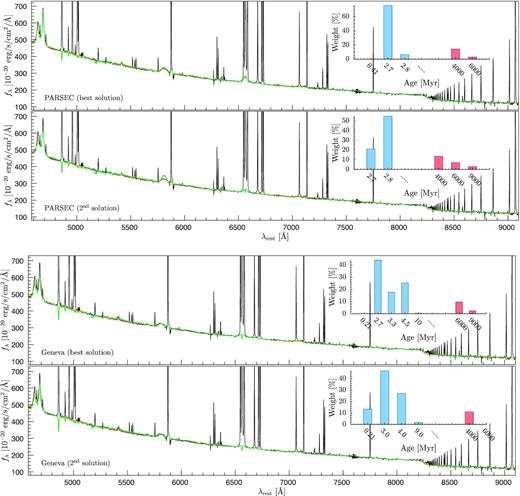
The double Zs solutions obtained from fitting Parsec and Geneva models to the Antennae H ii region A989. From the top to bottom panels, the final PDFs of Parsec (red) and Geneva (black) solutions, the Parsec best-fitting spectral model corresponding to the slightly super-solar Zs as shown in the respective PDF (in the top row), the Parsec second solution corresponding to a Zs of slightly sub-solar metallicity as shown in the respective PDF, the Geneva best-fitting spectral model corresponding to the slightly super-solar Zs as shown in the respective PDF, and the Geneva second solution corresponding to a Zs of slightly sub-solar metallicity. The insets show the age distributions corresponding to each solution.
The age–stellar metallicity degeneracy arises from the fact that with increasing stellar metallicity, the stellar continuum features start to appear at earlier ages. Therefore, there can be multiple age and stellar metallicity solutions to a given spectrum, with a higher metallicity solution predicting younger stellar ages than a lower metallicity solution. In the case of A989, both Geneva and Parsec models predict a best-fitting stellar metallicity that is slightly super-solar, as well as a second stellar metallicity solution that is slightly sub-solar. While the modelling of the WR features can be used to distinguish between the Parsec solutions clearly, the same cannot be used to discriminate between the Geneva solutions. In these cases, we assess ‘the best-fit model’ by considering the level of agreement between the best-fitting model and the observations over the wavelengths regimes containing the blue (4584–4811 Å) and red (5280–5861 Å) WR features, and the Paschen Jump (7827–8240 Å) as well as the telluric residuals prone 6875–7551 Å region. These are the wavelength ranges that generally show notable residuals. Another method of constraining multiple stellar metallicity solutions is through the best-fitting gas metallicity as the metallicity of the stars is unlikely to be significantly different from the metallicity of the gas from which they were formed. Therefore, the best-fitting gas metallicity can be used as a prior in the determination of the stellar metallicity. In the case of A989, however, all the best-fitting solutions appear to be largely similar in their distributions of age, metallicity, Te, and nH.
The degeneracy between nH and burst strength is mostly related to the lower versus higher ionization nature of the emission-line ratios used in the fitting. The line luminosity constraints based on higher ionization emission lines (e.g. [O iii] λ5007Å, [Ar iii] λ7135Å, [S iii] λ6312Å, and [S iii] λ9069Å) tend to bias nH (burst strength) towards higher (lower) values, and vice versa with lower ionization emission-line constraints (e.g. [N ii] λ6584, λ5755Å, [S ii] λ6717,31Å). Therefore, this apparent degeneracy is perhaps a tracer of the ionization structure of an H ii region.
4 THE MUSE ANTENNAE PROJECT
The observations of the Antennae galaxy were taken with the MUSE (Bacon et al. 2012) at the 8-m Very Large Telescope (VLT), with a 1 × 1 arcmin2 field-of-view between 2015 April–May and 2016 February–May. The wide-field mode set up with extended wavelength configuration (∼4600−9350 Å spectral coverage at relatively high resolution of R ∼ 3000) and 0.2 arcsec2 sky sampling was employed to observe the central regions and the tip of the southern tidal tail of the Antennae galaxy.
The MUSE observation strategy of the Antennae galaxy and the data processing are described in detail in Weilbacher et al. (2018). Briefly, most pointings composed on 1350s exposures taken with a spatial dithered pattern at fixed position angle, with several shallow extra pointings obtained at different position angles. Additionally, the observations of the central Antennae regions were supplemented with 200 s sky exposures. All exposures, except for one shallow central observation, were taken in clear or photometric conditions. The overall variation in seeing is approximately 0.5–1.2 arcsec, with an average in the sub-arcsecond regime. The depth of the observations vary across the central regions (fig. 2 of Weilbacher et al. 2018), and is taken into account through the relative weights assigned during the data processing, done consistently using the MUSE pipeline (Weilbacher et al. 2020) as outlined in Weilbacher et al. (2018), to produce data cubes of log and linear samplings. For the analysis presented in this study, we use the data cube with (linear) sampling of 0.2 arcsec × 0.2 arcsec × 1.25 Å voxel−1.
In Fig. 15, we show the Balmer decrement (i.e. Hα to Hβ flux ratio) and intrinsic star formation rate (SFR) surface density maps for the central regions of the Antennae galaxy. The Balmer decrement is an obscuration sensitive parameter, and its departure from the Case B theoretical value of 2.86 at an electron temperature of 104 K and an electron density of 100 cm−3 (Osterbrock & Ferland 2006) is an indication of the dust extinction along the line of sight. To construct the maps, we impose a signal-to-noise cut of 3 on both Hα and Hβ fluxes, and for the subset of cases where the spaxels show Balmer decrements <2.86, which can result from intrinsically low-reddening combined uncertainties in line flux calibration and measurement, we assume no dust obscuration. The H ii regions in the Antennae galaxy sample a wide range in dust obscurations and SFR surface densities, making the Antennae data ideal for studying the environments of young, massive stellar clusters formed in a violent gas-rich merger.
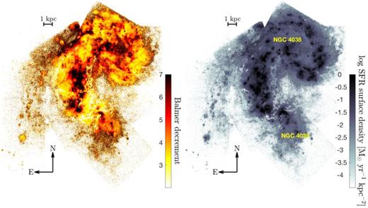
The Balmer decrement (left-hand panel) and log intrinsic Hα SFR surface density (right-hand panel) maps for the central regions of the Antennae galaxy, illustrating the wide-range range in dust obscurations and SFR surface densities sampled by the young, massive stellar clusters in the galaxy. The loop-like region west of the northern galaxy NGC 4038 is called ‘the western loop’, and the region between NGC 4038/39 that show significantly enhanced SFR surface densities is called ‘the overlap region’.
4.1 The H ii regions in the Antennae galaxy
For this study, we use the H ii regions discussed in Weilbacher et al. (2018), which are extracted using the dendrograms tool.9 Each H ii region represents a peak in the Hα flux map, which is then extracted down to the surface brightness level where the corresponding contours join, thus defining the size of the extracted region.
For the present analysis, we exclude the southern tidal tail and focus on the H ii regions in the central merger undergoing a ‘starburst’ following the Hα EW > 50 Å definition of Rodighiero et al. (2011). The 235 H ii regions meeting the EW criteria of Rodighiero et al. (2011) are shown in Fig. 16, overplotted on the SFR surface density map of the central region and colour-coded by their log Hα EW (left-hand panel), and overplotted on the 160-μm map of the Antennae galaxy (right-hand panel).
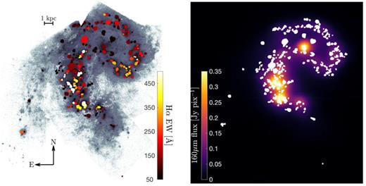
The H ii regions in a ‘starburst’ phase (i.e. Hα EW > 50 Å) overplotted on the SFR surface density map of the central regions of the Antennae galaxy and colour-coded by their average Hα EW (left-hand panel), and the same regions overplotted on the Herschel 160-μm map of the Antennae galaxy (right-hand panel). The maker size denotes the relative size of the H ii regions.
The right-hand panel of Fig. 15 and the left-hand panel of Fig. 16, together, show that the EW > 50 Å regions are generally characterized by log Hα SFR surface densities >−1 M⊙ yr−1 kpc−2, highlighting the extreme environments inhabited by young, massive stellar clusters. Similarly, the EW > 50 Å regions show a good correlation with the 160-μm distribution, particularly in the overlap region, demonstrating that the H ii regions selected for this analysis samples all the significant star formation in the central regions of the Antennae galaxy. We also show the distribution of the H ii regions selected for this study compared to that of all H ii regions with signal-to-noise ratio in Hα > 10 as a function three different properties in Fig. 17. Overall, the size and Balmer decrement distributions of the starbursting H ii regions largely overlaps with that of the full sample, suggesting the selected starbursting regions probe a wide range in environments. The distribution of [O iii] |$\rm {\lambda }$|5007/Hβ of starbursting regions is, however, skewed towards lower values with respect to the full distribution, which suggests that the selected starbursts are somewhat biased against lower metallicities (see also Fig. 10).
![From the left- to the right-hand panels, the distribution of all H ii regions in the Antennae galaxy compared that of the Hα EW > 50 Å regions as a function of size (indicated in terms of the total number of spaxels defining a given region), Balmer decrement, and [O iii]λ5007/Hβ flux ratio.](https://oup.silverchair-cdn.com/oup/backfile/Content_public/Journal/mnras/497/3/10.1093_mnras_staa2158/1/m_staa2158fig17.jpeg?Expires=1716411860&Signature=GYTSSxiPWSB7vD035mBA5gswlaRHGlIz-UEsUeSJ7x-qSXqOIMcbvwXpkBW2YGfECnc2MsmTX8epeARvldPUaxqgoD5h4J~cPAwHNtfVqEoUgAihJrm5vlmgUfcedXDmDF1mUDii4g5y6BO0~baGrBRXQOmKlNQeQaxaukB0YcV-x2DOquTQ3EJINa7MDJ8t-lMvwFD-Q3bUZocLAPq9-v3b27DFs8QzicV6l0r~k6OuFNPCXvUY8Sha8HQ5xVjWEcQlCegRQe9adrPgS-tnnfUce4lUAsT5E~jcTgjjhcXp~wub2zMxOLodD-z6zC2ENw12y-xU9fqI0ua3mjUazw__&Key-Pair-Id=APKAIE5G5CRDK6RD3PGA)
From the left- to the right-hand panels, the distribution of all H ii regions in the Antennae galaxy compared that of the Hα EW > 50 Å regions as a function of size (indicated in terms of the total number of spaxels defining a given region), Balmer decrement, and [O iii]λ5007/Hβ flux ratio.
4.2 The characterization of spatially correlated noise in the construction of integrated spectra
For each H ii region shown in Fig. 16, we create a signal-to-noise weighted integrated spectrum from the individual spectra (i.e. spatial pixels) defining that region. Likewise, we also create an integrated error spectrum by analytically propagating the error arrays of all the contributing spatial pixels. The analytically propagated error spectrum is, however, likely to underrepresent the true error due to noise in the adjacent pixels being spatially correlated, a consequence of the interpolation procedure used to obtain a regular grid of 0.2 × 0.2 arcsec2 in the final data cube. Therefore, to characterize the effect of correlated noise, we adopt the error analysis based on the full spectral fitting method described in García-Benito et al. (2015) and Husemann et al. (2013).
Neglecting any uncertainties or systematic deviations in models, the full spectral fitting analysis can provide a fair assessment of the accuracy of errors of a spectrum. In Fig. 18, we show the ratio the real noise (ϵreal) to the analytically propagated noise (ϵbinned) as a function of the spatial pixels contributing to each H ii region (grey lines) considered in this study. The ratio of ϵreal to ϵbinned is determined over the 4750−5600 and 6600−7600 Å windows. On average, each relation shows an initial increase in ϵreal to ϵbinned, followed by a flattening. We find that this behaviour is best described by the |$\epsilon _{\rm {real}} = \epsilon _{\rm {binned}} (1 + 0.18\sqrt{n})$| (indicated by the red line), which we use to scale the analytically propagated error spectrum of each region.
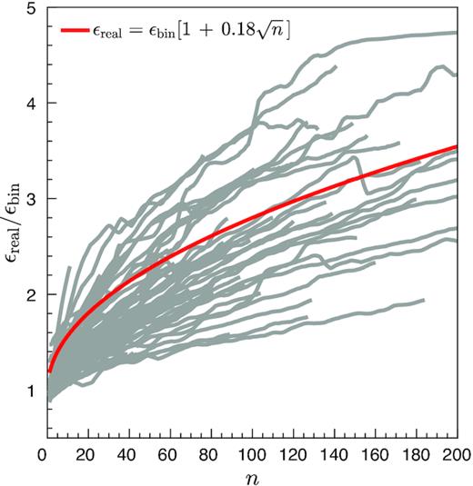
The characterization of the spatially correlated noise. The grey lines denote the individual relationships between the ratios of the real-to-analytically propagated noise (i.e. ϵreal to ϵbinned) versus the number of spaxels (i.e. n) obtained for the H ii regions considered in this study. The relation that best describe the data is shown in red. Note that this is not a best-fitting relation. It well describes the data in the high n region, but slightly overestimates the error in the low n regime.
5 THE CHARACTERISTIC PROPERTIES OF THE ANTENNAE H ii REGIONS
We apply the models described in Section 2 and the method outlined in Section 3 to the MUSE spectra of starbursting (i.e. Hα EW > 50 Å) H ii regions in the Antennae galaxies. The spectra of H ii regions are separately fitted with both the Geneva and Parsec model libraries to self-consistently derive stellar and gas metallicities, the age of the <10 Myr stars, the age of the dominant old (>10 Myr) stellar population, nH and Te, which we present in Figs 19 and 20, respectively. In each figure, from the left- to right-hand panel, top to bottom panel, the H ii regions are colour-coded by the age of the young (<10 Myr) stellar population, the old stellar population that dominate in lightweight in the 10−100 Myr, 100−1000 Myr and >1 Gyr range, the stellar and gas metallicity in the unit solar metallicity, nH and Te.
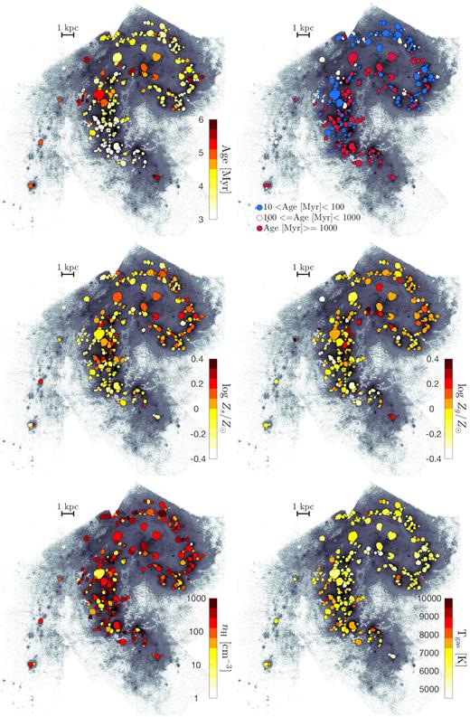
The Antennae H ii regions colour-coded by the light-weighted physical properties derived from fitting the Geneva high mass-loss models. From the left- to right-hand panels, top to bottom: the age of the young (i.e. <10 Myr) stellar population, the age of the dominant (in light-weight) old stellar population, the metallicity of the stars relative to solar metallicity, the metallicity of the star-forming gas relative to solar metallicity, nH in unit of cm−3 and Te in unit of K. The full catalogue of physical properties derived from fitting the Geneva models is available online.
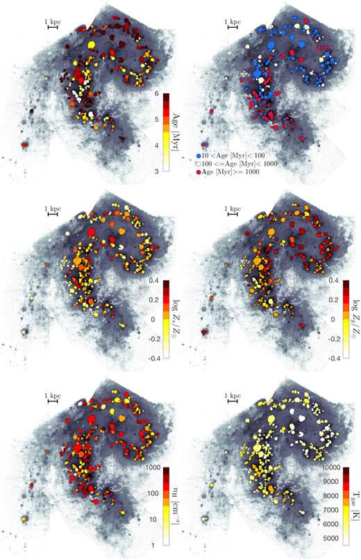
Similar to Fig. 19, but derived from fitting the Parsec model library. The full catalogue of physical properties derived from fitting the Parsec models is available online.
In the subsequent sections, we discuss the distribution of each property shown in Figs 19 and 20 and compare our results with the previous observations of the Antennae star-forming regions.
5.1 The stellar populations in the Antennae galaxy
For each starbursting region, we estimate the age of the ‘young’10 component using the light weights assigned to each <10 Myr spectral model contributing to the best-fitting solution. The dominant old11 stellar population, on the other hand, is determined by simply summing the lightweights of >10 Myr spectral models in 10−100 Myr, 100−1000 Myr, and >1 Gyr age bins.
5.1.1 The distribution of the <10 Myr old stellar population
The young stellar ages (Fig. 19, top left-hand panel) shows a trend, albeit weak, across the merger, where the youngest ages are localized to the overlap region, and some of the oldest ages are found in more extended H ii regions near the northeastern star-forming ridge (towards the centre of the northern galaxy NGC 4038). The western-loop of NGC 4038 also hosts young star-forming regions that, relative to the overlap region, appear to be slightly older. Compared to other regions, the H ii regions in the overlap region are experiencing a more significant enhancement in star formation as evident from both their atypically high Hα EWs (Fig. 16) and the average ∼3 Myr age distribution. The lack of a sizeable dynamical range in young stellar ages (Fig. 19, top left-hand panel) is likely a consequence of the fact that we are only showing the light-weighted ages of the young (<10 Myr) component with no regard to the light-weights assigned to any underlying >10 Myr stellar populations.
We find that the light-weighted young ages derived from fitting the Parsec models (Fig. 20 top left-hand panel) show broadly the same qualitative trends as Geneva. Overall, there is a good agreement between the Geneva and Parsec results. The subset of H ii regions where the respective Parsec and Geneva-based light-weighted young ages differ by more than their 1σ errors are shown in the left-hand panel of Fig. 21. As can be seen, the young ages derived from fitting Parsec and Geneva libraries are consistent within error for a significant fraction of the H ii regions. Interestingly, however, Parsec models tend to yield young ages for star-forming regions that are mostly older than the Geneva models (Fig. 21 left-hand panel inset). As a consequence, the Parsec versus Geneva residual map of the ages shown in Fig. 21 is biased somewhat towards positive differences. Moreover, the PDFs derived from fitting Parsec models, on average, show larger dispersions, which, in turn, yields larger uncertainties for Parsec derived physical properties than the Geneva-based properties. We discuss this in detail in Appendix B. Briefly, a direct comparison between the Geneva and Parsec PDFs derived for 20 H ii regions across NGC 4038/39 is presented in Fig. B1 in Appendix B, which shows that in most cases the Zg derived from fitting Parsec models are biased towards slightly super-solar metallicities than Geneva. Also, the Parsec PDFs of Zs are generally broader than that of Geneva.
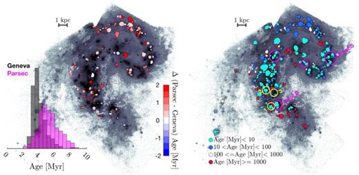
Left-hand panel: The residual map showing the differences in light-weighted young (<10 Myr) ages derived from fitting Geneva HML and Parsec models. The H ii regions are colour-coded by their differences, and only those that show differences more significant than their respective 1σ errors are shown. The inset compares the Geneva (black) and Parsec (magenta) distributions of light-weighted ages of all H ii regions selected for this study. Right-hand panel: the H ii regions colour-coded by the age of the dominant stellar population derived from the fitting Geneva HML models. The dominant age is now determined by considering the light-weights of individual spectral models constituting to a best-fitting model over four age bins, including the youngest ages (i.e. <10 Myr, 10−100 Myr, 100−1000 Myr, and ≳1 Gyr). The H ii regions indicated within circles are some of the regions that have been widely studied in the literature, which we discuss in detail in Section 5.1.3. The distribution of dominant ages derived from fitting Parsec models (not shown here) is in agreement with the Geneva result shown.
5.1.2 The distribution of the >10 Myr stellar population
In Figs 19 and 20 top right-hand panels, we show the distributions of the dominant old (>10 Myr) stellar populations contributing to the Geneva and Parsec best-fitting spectral models. Both Parsec and Geneva ages show a clear dichotomy in the distribution of the old stellar population across the merger. The H ii regions in the northern galaxy NGC 4038 appear to host an underlying old stellar population of between 10 and 100 Myr in age, whereas the regions in the southern NGC 4039 show signs of the presence of a much older, an ∼Gyr-type, underlying stellar population. The spectral features of an ∼Gyr versus a few Myr stellar population are distinct. Therefore to demonstrate further that the starbursting regions in the two galaxies host two distinctive old stellar populations indeed, we show the best-fitting spectral models for two H ii regions, one residing in NGC 4038 (H ii region A654) and other in NGC 4039 (H ii region A1365), in Fig. 22. The spectrum of A654 shows more pronounced absorption features, particularly towards the bluer wavelengths, that rivals in strength with Balmer absorption features. In comparison, however, the same features in the A1365 spectrum are less prominent, although its blue continuum is more enhanced than that of A654.
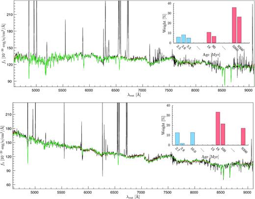
The Geneva HML best-fitting spectral models (shown in green) obtained for the Antennae H ii regions A654 (top panel) and A1365 (bottom panel). The region A654 resides in the southern galaxy NGC 4039, and show distinct continuum spectral features common to ∼1 Gyr stellar population. The region A1365 is part of the northern system NGC 4039, and show clear continuum features common to stellar populations of few tens of million years old. The Parsec best-fitting spectral models (not shown here) also clearly discriminate these distinct stellar populations and are in agreement with the Geneva result. The best-fitting models adjusted with a fit to the residuals are also shown in red to highlight that in most cases the best-fitting model alone provides a good description of the spectra of Antennae H ii regions without needing any form of adjustment. The insets show age distributions corresponding to each best-fitting solution.
For completeness, we also show the distribution of the ages of the dominant stellar populations in the Antennae, including the <10 Myr populations, in the right panel of Fig. 21. The dominant ages of the H ii regions residing in the overlap region and the southern portion of the western loop appear to be <10 Myr, the northern portion of the western loop appears to be inhabited by H ii regions with stellar populations in the 10−100 Myr age range, while most H ii regions in NGC 4039 show signatures of an ∼Gyr-old stellar population. Qualitatively, the trend in the distribution of the dominant stellar populations across the Antennae is similar to that observed for the light-weighted young stellar ages (Figs 19 and 20).
It is interesting to note that the H ii regions in the northern portion of the western loop appear to have an underlying dominant stellar population of 10−100 Myr in age. The Parsec light-weighted young ages of these regions are notably older than those based on the Geneva (Fig. 21, left-hand panel).
5.1.3 Comparison with previous age estimates of the H ii regions in the Antennae
Zhang, Gao & Kong (2010) compared the broad-band spectral energy distributions for 34 24-μm dust emission peaks across the Antennae to determine the SFH along the merging discs. Based on the large ratios of 24μm to 8μm observed across the overlap region as well as the strong ultraviolet emission detected over the western loop, they conclude the overlap region and western loop to be the most intense star-forming sites in the Antennae. Between the H ii regions in the overlap region and the western loop, Zhang et al. (2010) report that the regions in the western-loop are in a relatively later stage of star formation than those in the overlap region, in agreement with our findings above.
Using the HST Advanced Camera for Surveys observations of the Antennae in the UBVIHα filters, Whitmore et al. (2010) predict the ages, extinction and masses for a large number of star clusters across the mergers using the population synthesis models of Charlot & Bruzual (the 2007 suite of models; see also Bruzual & Charlot 2003). For a part of the overlap region, called Knot B in their study (also indicated in the right-hand panel of Fig. 21), they find that except for a single 10−50 Myr cluster lying at the heart of the Hα shell, the rest of Knot B is dominated by <10 Myr clusters with a majority <5 Myr in age. A direct comparison between our work and that of Whitmore et al. (2010) is difficult as our sample comprises of starbursting H ii regions, which likely encompass many individual star clusters. None the less, the ages reported by Whitmore et al. (2010) for a large fraction of the young star clusters embedded in the vast H ii region within Knot B (right-hand panel of Fig. 21) agree with the age estimates derived for that region in this study. Moreover, Mengel et al. (2005), Snijders (2007), and Brandl et al. (2009) have also studied the young H ii region within Knot B. The ages they report are between 2.3 and 4 Myr, again in agreement with the result of this study.
The H ii regions to the left of Knot B (the yellow circle labelled 1 in the right-hand panel of Fig. 21) have been reported to have ages between 2.3 and 4 Myr (e.g. Mengel et al. 2005; Gilbert & Graham 2007; Snijders 2007; Brandl et al. 2009), for the regions within circle-2, ages between 1 and 4.9 Myr (Mengel et al. 2005; Gilbert & Graham 2007; Snijders 2007; Brandl et al. 2009; Whitmore et al. 2010) and for circle-3, ages between 3 and 5.7 Myr (right yellow circle Mengel et al. 2005; Gilbert & Graham 2007; Snijders 2007). Except for the last region, which is not bright enough in Hα to be considered a starburst based on its Hα EW, the ages we derive for the rest are within the age ranges reported in the literature. There is also a good agreement between the Geneva and Parsec predictions of these regions.
For the older cluster within Knot B, to the right of the large H ii region, Whitmore et al. (2010) estimate an age of 10−50 Myr. We find that the light-weighted age of the young component of this region to be ≲5 Myr, however, its spectrum is similar to that shown in the top panel of Fig. 22, implying the presence of an underlying stellar population of around a Gyr or so in age. Interestingly, the spectra of most of the H ii regions inhabiting NGC 4039 show signs of an ∼Gyr−type underlying population, which we discuss below.
We have also indicated ‘Knot S’ studied by Whitmore et al. (2010) in the right-hand panel of Fig. 21. For this region, Whitmore et al. (2010) find a mixture of ages, with <10 Myr clusters dominating in number. The youngest clusters (<5 Myr) in the region appear to be mostly positioned to the left of the highest star formation peaks, with the 5−10 Myr clusters scattered across the region, which Whitmore et al. (2010) interpret as a sign of the progression of star formation towards the dust reservoir. They also find a scattering of 10−100 Myr clusters through much of the region. We find evidence for a similar variation in ages in the Geneva and Parsec distributions of light-weighted young ages (Figs 19 and 20), largely in agreement with the results of Whitmore et al. (2010). However, we remind the reader, again, that we cannot perform a direct comparison with the Whitmore et al. (2010) results as the H ii regions shown may encompass several star clusters.
Magenta circles (without labels) in Fig. 21 indicate two other knots studied by Whitmore et al. (2010). According to their study, many of the star clusters residing within these knots have ages <5 Myr, with 5−10-Myr old clusters positioned approximately at the centres of the peaks in star formation. Also, for some of the star clusters within the two circles, Bastian et al. (2009) report ages between 3.16 and 6.3 Myr. According to this study, some to the H ii regions within these circles have Geneva-derived ages <4 Myr and Parsec-derived ages in the range 4−5 Myr, which are broadly in agreement with Bastian et al. (2009) and Whitmore et al. (2010), though, there are some discrepancies between the Geneva and Parsec estimates as can be seen in their residual map (Fig. 21).
On the old stellar populations in the Antennae, the numerical modelling studies (e.g. Barnes 1988; Mihos, Bothun & Richstone 1993) of the merger suggest that the first encounter between the two progenitors occurred ∼200−400 Myr ago. In support of this time-frame, several observational work (e.g. Whitmore et al. 1999; Zhang, Fall & Whitmore 2001; Bastian et al. 2009; Whitmore et al. 2010) find evidence for the existence of intermediate-age clusters scattered throughout the merger, primarily across the northeastern star formation ridge of NGC 4038, with ages varying between 100 and 600 Myr.
In this analysis, we also see evidence for the presence of underlying old stellar populations in the starbursting regions. Our models predict both intermediate-age and older stellar populations, and intriguingly, there seems to be a dichotomy between the distribution of these two populations. The intermediate-age populations, comprising mainly of 10−100-Myr regions as well as some between 100 and 1000 Myr, are scattered across NGC 4038, including the overlap region, whereas the spectra of the H ii regions in NGC 4039 show signs of a much older, around Gyr or so in age, population. In comparison, the distribution of the intermediate-age population across regions belonging to NGC 4038 appears to be similar to that reported by Whitmore et al. (1999). In terms of ages, Whitmore et al. (1999) report an age of ∼100 Myr for the H ii regions residing mostly around the northeastern ridge, which is broadly consistent with the ages of 10−100 Myr found for that region in this study. Whitmore et al. (1999) also find a second older, ∼500 Myr, population, mainly residing in the tidal tails, which they associate with the initial encounter between the progenitors. In our study, for the two large H ii regions out of the four in the tidal tails that are currently in a starburst phase, we find dominant old ages of around ∼Gyr. We also find evidence for the existence of ∼Gyr−type populations in starbursting regions that appear to belong to the southern system NGC 4039.
Finally, we note that it is challenging to constrain the ages of the old stellar population accurately from the current analysis alone. For the determination of young ages (i.e. <10 Myr), for example, we have utilized constraints from stellar and nebular continua as well as nebular lines, adding thorough constraints on young ages, whereas the old stellar populations are constrained only using continuum spectral features. The age-selective dust attenuation may also be necessary for better constraining old stellar populations, which we have not considered in this analysis (see Section 5.6 for a discussion). This is one of the main reasons as to why we report old stellar population ages in bins of 10−100 Myr, 100−1000 Myr, and ≳1 Gyr. Another being that, as discussed in Section 2.3 and demonstrated in Figs 19 and 20, the ages derived are dependent on the isochrones used.
5.2 The metallicities of the stars and the star-forming gas in the Antennae
The middle panels of Figs 19 and 20 present the H ii regions colour-coded by their stellar and gas metallicities (in units of solar metallicity) derived from fitting Geneva and Parsec model libraries, respectively.
5.2.1 The stellar metallicity
We find that, on average, both Geneva HML and Parsec best-fitting light-weighted stellar metallicities for the H ii regions in the Antennae are around solar. There is a weak trend towards slightly super-solar stellar metallicities evident in the Geneva results (Fig. 19, middle left-hand panel), which is, however, not apparent in the Parsec distribution (Fig. 20, middle left-hand panel).
In Fig. 23 left-hand panel, we show the agreement between Geneva and Parsec derived stellar metallicities. As in Fig. 21, only the H ii regions with differences in stellar metallicities more significant than their 1σ error overlap are plotted. Overall, there is a good agreement between the predictions of the two model libraries. The inset in the left panel of Fig. 23 compares the Geneva versus Parsec derived metallicities for all H ii regions, and both distributions indicate similar broad dispersions. This is perhaps a result of the age − stellar metallicity degeneracy yielding different potential stellar metallicity and age solutions, and thus increasing the dispersion of the stellar metallicity PDFs of the best-fitting solutions (Fig. B1). As discussed in Section 3.4, the presence of prominent WR features and the Paschen jump in the nebular continuum can alleviate the effects of the age − stellar metallicity degeneracy to an extent.
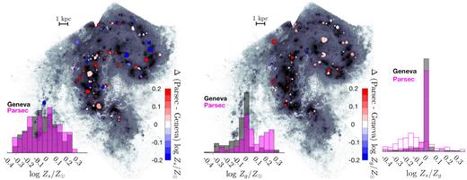
Residual maps showing the differences in stellar (left-hand panel) and gas (middle panel) metallicities derived from fitting Geneva HML and Parsec models. The H ii regions are colour-coded by their differences, and only those regions that show differences more significant than their respective 1σ uncertainties are shown. The insets compare the Geneva (black) and Parsec (magenta) distributions of Zs and Zg of all H ii regions selected for this study. The distributions of Zs − Zg are shown in the right-hand panel. The open magenta histogram presents the Parsec Zs−Zg distribution, which shows a peak towards lower values, suggesting a higher enrichment in gas relative to stars in most H ii regions. Within the uncertainties, however, Zs and Zg are mostly in agreement as shown by the filled histograms.
5.2.2 The gas metallicity
In the middle-right panels of Figs 19 and 20, we show the distributions of the light-weighted gas metallicities derived from fitting the Geneva and Parsec model libraries. Both sets of models broadly predict solar-like metallicities for the H ii regions in the Antennae, although, on average, the Parsec predictions appear to be slightly biased towards super-solar values. The Geneva versus Parsec residual map is shown in the middle panel of Fig. 23, which demonstrate that within 1σ error, the two model predictions for a significant fraction of the H ii regions are indeed consistent.
There is a trend in the distributions of gas metallicities across the merging discs. Both models predict the star-forming gas in the H ii regions around the western loop to be more enriched than those inhabiting the overlap region. The H ii regions in the overlap region and NGC 4039 show a mix of metallicities in the range between slightly sub- to super-solar. The inset in the middle panel of Fig. 23 present a comparison of the Geneva and Parsec derived gas metallicities for all H ii regions, which shows that solar-like gas metallicities characterize a significant fraction of the H ii regions in the Antennae, supporting our earlier assertion. Interestingly, the Parsec distribution shows a more distinct bimodality than the Geneva, reflecting the fact that the Parsec derived metallicities of H ii regions across the western loop indicate, on average, a slightly greater enrichment that the respective Geneva metallicities (the right-hand panels of Figs 19 and 20).
In most of the previous figures, we referred to the common expectation that metallicity of stars is likely similar to that of the star-forming gas. In the right-hand panel of Fig. 23, we present a comparison between stellar and gas metallicities. The filled (open) histograms denote the Zs/Zg distributions with (without) their respective 1σ uncertainties taken into account. Within uncertainties, both Geneva and Parsec distributions are centred around zero, indicating a good agreement between stellar and gas metallicities for a majority of H ii regions. Notably, both distributions, however, show a tail extending towards low Zs/Zg, pointing to a higher enrichment in gas relative to stars in some H ii regions. It is plausible for the stellar metallicity to be somewhat lower than that of gas, especially if the region is in a later stage of star formation. These differences, however, could also be an artefact of the age–stellar metallicity or dust degeneracies discussed earlier.
5.2.3 Comparison with previous metallicity estimates for the H ii regions in the Antennae
Mengel et al. (2002) report solar-like stellar metallicities for six H ii regions in NGC 4038 based on an analysis of the metallicity-sensitive Mg i line at 8806.8 Å. Similarly, Lardo et al. (2015) measure Fe, Mg, Si, and Ti abundances for three super star clusters (two are part of the western loop, and the third resides in the northeastern ridge) and infer slightly super-solar metallicities of ∼0.07 ± 0.03. Lardo et al. (2015) also calculate direct metallicities (i.e. gas-phase metallicities), which are consistent with being slightly super-solar.
Bastian et al. (2009) derived metallicities for 16-star clusters in the Antennae from a comparison of observed Balmer and metal line strengths with SPS models, as well as using strong emission lines where available. Out of the 16 star clusters, 15 are part of the central merger, with four residing in NGC 4039 and two of which are young, and the rest distributed mostly around the western loop of NGC 4038 and five of which are young. For all these star clusters, Bastian et al. (2009) infer metallicities that are, on average, solar to super-solar. The metallicities of the H ii regions that these star clusters are members of likely similar.
Overall, the observations of solar to slightly super-solar stellar and gas metallicities for the star-forming regions are consistent with the results of this analysis. Finally, utilizing the observations of Bastian et al. (2009) and Lardo et al. (2015) find a flat abundance gradient across the merger. In this analysis, however, we find a weak trend; the gas metallicities of H ii regions in the western loop appear to be more metal-rich than those in the overlap and NGC 4039 regions. This trend is, however, not evident in the distribution of stellar metallicities.
5.3 On the distribution of the electron densities and temperatures in the Antennae
The light-weighted electron densities and temperatures derived from fitting Geneva and Parsec models are shown in the bottom left- and right-hand panels of Figs 19 and 20.
By large, the derived nH values are within the 100−1000 cm−3 range, and we find no clear trend in their distribution across the central regions of the merger. As discussed in Section 3.4, however, most nH PDFs show double peaks, which appear to be associated with the higher and lower ionization nebular constraints used in the fitting. The Te of H ii regions are, on average, centred around 7000 K, and as with nH, show no clear variation across the central merger.
In Appendix C, we present a comparison between the PyNeb-based estimates of nH and Te and those derived from fitting the Geneva and Parsec models. On average, the majority of the model-based nH values are higher than the PyNeb estimates, with a small subset of H ii regions having nH lower than the respective PyNeb values. In contrast, the model-based light-weighted Te is lower than that estimated with PyNeb.
5.4 On the distribution of burst strengths in the Antennae
The final parameter of the model H ii regions is the strength of the starburst. This parameter is very sensitive to the ionization structure of an H ii region, and as the ionization structure is not homogeneous throughout a region, it can be challenging to constrain the burst strengths. For example, Figs 13 and 14 illustrate the typical PDFs derived for burst strengths, which tend to show several distinct–distinct peaks.
The range in burst strengths probed by the current library of models is 102−104 M⊙, assuming a fixed radius for the model H ii regions (Table 2). The main reason for choosing this range in burst strengths is that the strength of a burst is directly proportional to U (equation 2). As such, increasing the strength significantly tend to yield high U values (i.e. log U > –0.5) for ages around ∼1 Myr, which have not been explored much in the literature. Given the radius dependence of the burst strength parameter, to extract the most likely burst that would have formed a given H ii region in the Antennae, the above range in burst strengths needs to be compensated for the difference in radii following equation (2).
Overall, almost all H ii regions studied show a preference for starbursts of >104 M⊙ in strength. Whitmore et al. (2010) find masses in the 104−107 range for the star clusters in the Antennae, similar to the range in burst strengths derived in this study. It is, however, difficult to perform a direct comparison with Whitmore et al. (2010) work as their work is focused on star clusters and largely use photometry in the determination of masses. In contrast, our work focus of H ii regions that likely consist of several star clusters and principally utilize the emission-line ratios in constraining the strength of the starburst that likely formed a given H ii region.
5.5 Correlations between properties
To explore the correlations between different physical properties, we plot the stellar and gas metallicities, and the light-weighted young ages derived from fitting the model libraries as a function of various properties, e.g. Hα EW, Balmer decrement, Hα luminosity per unit spaxel, Hα SFR, Hα SFR surface density and stellar mass of H ii region estimated by summing the masses of star clusters within that region, in Fig. 24. The star cluster masses are drawn from the catalogue of Whitmore et al. (2010).
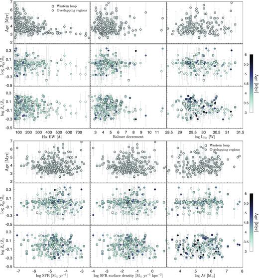
The model-based properties (e.g. light-weighted young age, and gas and stellar metallicities) as a function of Hα equivalent width in unit of Å, Balmer decrement, Hα luminosity in unit of W spaxel−1 (top set of nine panels), SFR in unit of M⊙ yr−1, SFR surface density in unit of M⊙ yr−1 kpc−2, and cluster mass in unit of solar masses (bottom set of nine panels). The circles and squares denote the H ii regions residing in the overlap region, including the southern NGC 4039, and the western loop, respectively, and the colour-code indicate the light-weighted young ages of the H ii regions.
Different marker types are used to distinguish between the H ii regions in the overlap region (including NGC 4039), and those residing in the western loop. The data points are colour-coded by the light-weighted young ages. Except for weak trends apparent in the age versus Hα EW and the age versus Hα luminosity per unit spaxel plots, there appear to be no strong correlations between these properties. In the case of age versus Hα EW, the H ii regions show a trend where most regions with high Hα EWs are characterized by younger ages, and as expected, this trend is more notable in the H ii regions residing in the overlap region than those in the western loop. Similarly, the H ii regions in the overlap region show preference for high Hα luminosities than those residing in the western loop.
5.6 Potential caveats to keep in mind
There are several potential caveats to the suite of models used in this analysis.
The Lyman Continuum (LyC; λ < 912 Å) photons leakage from H ii regions. Weilbacher et al. (2018) find that a significant fraction of H ii regions in the Antennae galaxy is leaking LyC photons at various levels. In this analysis, however, we construct model H ii regions assuming no leakage of LyC photons, which likely increase the dispersion of the reported properties.
Age-selective dust attenuation. During the model-fitting process, we have made the implicit assumption that both the young and old stellar populations are attenuated to the same extent. Since the massive, hot stars are born enshrouded in molecular clouds, which are dissipated during the lifetime of an H ii region, dust attenuation can be age selective (Charlot & Fall 2000; Tuffs et al. 2004). While we have not explored this aspect extensively in this analysis, given that we are targetting starbursting H ii regions, the uncertainties arising from the lack of age-selective attenuation corrections are likely minimal. The likely consequence of not including age-selective attenuation is a bias in the selection of old stellar populations towards older ages.
Stellar rotational mixing and binary evolution of massive stars. The current library of models for starbursts does not consider the stellar evolutionary scenarios that take the effects of binary evolution and stellar rotation into account. These scenarios are critical for the modelling of massive star formation. The stellar evolutionary models, like bpass (Eldridge & Stanway 2009) and mesa (Choi et al. 2016), allow these scenarios to be incorporated into the models of H ii regions, and their evolutionary predictions for massive stars can be vastly different from those of single stellar evolutionary models. bpass, for example, predicts ∼100 Myr duration for the WR stars in contrast to an ∼4−5 Myr durations predicted by the single stellar models (Eldridge et al. 2017). As discussed in Section 3, the fitting process derives constraints from both the stellar + nebular continua and emission-line luminosities of a given spectrum. The WR features, in particular, provide strong constraints on young stellar ages and metallicities. The bpass SSPs show presence of WR bumps over a long period, with features changing rather more slowly in appearance than in the case of SSPs based on single stellar models. For a fixed metallicity and age, the WR features appear to be stronger in the SSPs based on single-star models than in binary models. Without performing a full model fitting with bpass SSPs, it is difficult to say with certainty the extent of the changes to the light-weighted ages and metallicities reported in this study. Based on the differences between the bpass and starburst99 SSPs mentioned above, however, it is likely that bpass based ages would be biased towards older stellar populations, and metallicities towards higher values.
The incorporation of binary models in our fitting procedure is in theory feasible but it does open up a large parameter space, moreover it is also challenging to find high-resolution stellar libraries that adequately describe binary interactions. Therefore, before using these evolutionary scenarios for constructing models of H ii regions, further exploration is needed to understand not only the best ways of constraining models, but also the adjustments needed in fitting routines to minimize computational costs.
The stochastic sampling of the stellar IMF. Ordinarily, starbursts of <10 000 M⊙ are likely to produce stochastic stellar populations, whereas those >1 × 10⁵ M⊙ yield mostly-to-fully sampled IMF. In this analysis, we assume that the IMF is fully sampled, and as most of the H ii regions in the Antennae are massive star-forming regions, the effects of stochasticity are likely minimal. There are, however, some regions with masses ≲ 105 M⊙, and these regions could have stochastic massive stellar populations. The suite of models described in this paper is not equipped to address stochastic IMF sampling, the effects of which will likely increase the dispersion of the physical properties reported for those regions. According to Paalvast & Brinchmann (2017), in the presence of significant stochasticity, the mean trend would be for the emission lines to appear to come from slightly more enriched gas than they would if the IMF was fully sampled.
6 SUMMARY
In this paper, we discuss a methodology to exploit the full spectrum (continuum and emission lines) of an H ii region. Our goal is to be able to model all the spectral features contained in a spectrum, and thereby extract information on stellar and gas metallicity, age of the stellar population, Te and nH, and the strength of the zero-age starburst that would have produced the region, simultaneously.
To achieve this goal, first, we develop a suite of comprehensive self-consistent and time-dependent models for characterizing starbursting H ii regions. The model H ii regions are defined by five physical parameters; the effective temperature and age of the stellar population, chemical abundance, ionization parameter, and density. One of the most important features in spectra of starbursts is the WR feature, and any model-based methodology that attempts to provide a physical description for a starbursting region must be able to reproduce these features. Therefore, in our construction of the stellar models, we use the latest information on the stellar and WR libraries, and WR classifications. Moreover, we employ two different stellar isochrones; the Geneva isochrones that are generally preferred for the modelling of massive stars, and the latest Parsec isochrones, in order to explore possible systematics arising from the different implementations of stellar evolution.
Secondly, we discuss a potential model-fitting strategy that allows us to exploit the full spectrum, and thereby extract a number of physical properties simultaneously. The fitting procedure is two-fold. In the first instance, we fit the observed (stellar and nebular) continuum to extract the models for the unique underlying stellar populations contributing to an SFH of a region. Then, we use the age distribution of the extracted models and their light-weights to construct a nebular model, and all of this is done as a function of the model library parameters.
By applying the methodology summarized above to the MUSE spectra of the highly star-forming regions (i.e. Hα EW > 50 Å) in the Antennae galaxy, we were able to extract the following light-weighed physical properties; the young (<10 Myr) age of the stellar populations, the ages of the dominant underlying old (i.e. >10 Myr) stellar populations, stellar and gas metallicities, Te and nH. The distributions of each of these properties corresponding to the Geneva- and Parsec-based model libraries are shown in Figs 19 and 20.
Thanks to its proximity, the Antennae galaxy is well studied, and there is abundant literature on the properties of its H ii regions. In Section 5.1.3, we present a detailed comparison between the ages of the stellar populations derived in this study and the literature to date. Likewise, a thorough discussion of the stellar and gas metallicities obtained from full-spectrum fitting compared to other methods employed in the literature is presented in Section 5.2.3. In summary, we find that the H ii regions with the youngest ages lie in the overlap region between the two merging discs. The H ii regions in the western-loop of NGC 4038 also appear to host young stellar populations, although, their ages are older than those in the overlap region. Our results are consistent with a number of studies have also made similar observations (e.g. Mengel et al. 2005; Snijders 2007; Whitmore et al. 2010; Zhang et al. 2010). For the stellar and gas metallicities, we find around solar-like values for the starbursts in the Antennae, which is again consistent with the literature (e.g. Bastian et al. 2009; Lardo et al. 2015).
For the Antennae starbursting regions, we derive Te, on average, around ∼7000 K, and average nH of slightly >100 cm−3, and again, there appears to be no significant trend in their distributions. A detailed discussion on the distribution of these parameters as well as on the comparisons between the Te and nH derived from the full-spectrum fitting method and that estimated from widely used PyNeb software (Luridiana et al. 2015) is presented in Section C.
The zero-age burst strengths derived for almost all H ii regions studied are in the range 104−107M⊙. The burst strength is highly sensitive to the ionization structure of an H ii region, as such it is more difficult to constrain than the other parameters. While the range in burst strength derived is similar to that found by Whitmore et al. (2010) for the star clusters, a one-to-one comparison cannot be performed given the differences between the methodologies used. Refer to Section 5.4 for a discussion on the burst strength parameter.
ACKNOWLEDGEMENTS
We thank the anonymous referee for the constructive comments that have helped us to refine the analysis presented in this paper. MLPG acknowledges the support from European Union’s Horizon 2020 research and innovation programme under the Marie Sklodowska-Curie grant agreement no 707693. PMW was supported by BMBF Verbundforschung (project the Multi-Unit Spectroscopic Explorer-Narrow Field Mode, grant 05A17BAA). AM-I acknowledges support from the Spanish MINECO (Ministerio de Economía y Empresa) through project AYA2015-68217-P.
Data used in this paper are based on observations collected at the European Organisation for Astronomical Research in the Southern Hemisphere under ESO programs 095.B-0042, 096.B-0017, and 097.B-0346.
This work used the DiRAC@Durham facility managed by the Institute for Computational Cosmology on behalf of the STFC DiRAC HPC Facility (www.dirac.ac.uk). The equipment was funded by BEIS capital funding via the Science and Technology Facilities Council (STFC) capital grants ST/K00042X/1, ST/P002293/1, ST/R002371/1, and ST/S002502/1, Durham University and STFC operations grant ST/R000832/1. DiRAC is part of the National e-Infrastructure.
DATA AVAILABILITY
Data used in this paper are based on observations collected at the European Organisation for Astronomical Research in the Southern Hemisphere under ESO programs 095.B-0042, 096.B-0017, and 097.B-0346, and are available in the ESO archive. The data products resulted from the analysis presented in this paper are available in its online supplementary material.
Footnotes
The large number of iron-line transitions (Fe iv, Fe v, Fe vi) form a pseudo-continuum in the ultraviolet dominating the spectral energy distribution. The iron group line-blanketing is, therefore, important for reproducing the observed spectra of WR stars, particularly, WC subtypes (Gräfener, Koesterke & Hamann 2002)
The highest metallicity considered is Z ∼ 0.04.
The PARSECv1.2S library is downloaded from the CMD3.1 web interphase (http://stev.oapd.inaf.it/cgi-bin/cmd)
This is partly a result of many of the strong coolants been suppressed above their critical density
The intensity ratios are defined as [O iii] (I(4959) + I(5007))/I(4363), [N ii] I(5755)/(I(6548) + I(6583)) and [S iii] I(6312)/(I(9532) + I(9069)) (Peimbert et al. 2017), for the reason that, for example in [O iii], an excitation to the 1D results in the emission of a photon in either λ5007Å or λ4959Å with a relative probability of 3 to 1 (Osterbrock & Ferland 2006). However, the [O iii] λ4363Å and [S iii] λ9532Å are outside the MUSE wavelength coverage, and in the fitting, we tie I(6548) to I(6584), so only the I(5755)/I(6583) and I(6312)/I(9069) are shown.
We emphasis that this is only a slight bias and is largely seen in the fitting of spectra that show prominent WR features. Otherwise, the young ages derived from fitting Parsec models appear to be biased toward older ages. See Appendix B for a discussion.
Part of the astrodendro package from http://dendrograms.org.
Note that we define ’young’ stellar population to be a one that has a nebular model, which essentially means a <10 Myr population
'old’ is broadly defined to be any stellar population >10 Myr in age
REFERENCES
APPENDIX A: ON THE MODELLING OF WR FEATURES
In Sections 2.1.2 and 2.3, we discuss the selection of the spectra from the PoWR library to input into starburst99, and the properties of the generated SSPs, respectively. Out of a total of 1385 spectra provided in the PoWR WC, WNE, and WNL libraries, we remove four spectra from the PoWR WC library (two from the Galactic and two from the LMC) in order to generate stellar templates in cooperation with the Geneva HML isochrones with WR features similar to those that have been observed in the spectra of starbursting H ii regions. How the SSPs of solar metallicity change as a result of this small change to the WC library is shown in Fig. A1.
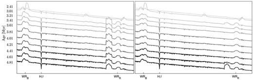
With (left-hand panel) and without (right-hand panel) the inclusion of the PoWR Galactic WC spectra 12–18 and 12–19 in the starburst99 synthesis of stellar evolution guided by the Geneva isochrones.The inclusion of these spectra produce a pronounced blue emission peak of the red WR feature, which is a feature the WC9 WR stars.
In the left-hand panel of Fig. A1, we show the stellar templates produced by incorporating the full Galactic PoWR library, and on the right-hand panel, the stellar templates generated by removing the WC spectra 12–18 and 12–19 from the Galactic library. By removing the spectra, the significantly enhanced blue component of the red WR bump, a strong signature of WC9 WR stars, evident across a wide range of young ages is suppressed. Likewise, we remove the 12–21 and 12–22 spectra from the PoWR LMC WC library, which, again, act to reduce the enhancement of the blue emission peak of the red WR bump.
These modifications to the PoWR WC libraries are motivated by the fact that the observations of H ii regions and galaxies in the nearby Universe do not show such heightened WC9 WR features. Also, the stellar metallicity effects can be crucial in the formation of different subtypes of WR stars. For instance, Sander et al. (2012) illustrate that the WC4 stars in the LMC are significantly brighter than their Galactic counterparts for the same mass-loss rates, and conclude that the WC4 stars in the LMC likely have higher current mass than the Galactic WC4 WR stars, as well as higher luminosities in order to drive the same mass-loss.
It is worth re-iterating that, as discussed in Section 2.1.2, the mass-loss rates from the stellar isochrones play a significant role in the selection of the WR spectra. The enhancement of the blue peak of the red WR bump appears to be primarily related to the use of the Geneva HML isochrones. The mass-loss rates, among to other parameters, derived from the PARSEC isochrones, on the other hand, do not lead to a substantial enhancement of the features of the red WR bump. However, for consistency, we have used the modified PoWR library throughout.
Finally, as evident in Fig. A1, the removal of the spectra also affect other WR features. In particular, the blue component of the blue WR feature is somewhat suppressed at certain ages.
APPENDIX B: PARSEC VERSUS GENEVA
In Fig. B1, we present a comparison between Geneva (black dashed) and Parsec (brown filled) fits for 20 H ii regions in total; 10 (top panels) distributed across the western-loop and the rest across the overlap region and NGC 4039. On average, the Parsec-based light-weighted young ages are relatively older, and the dispersion is larger than the respective Geneva-based values. We discuss some of the potential reason for these discrepancies below.
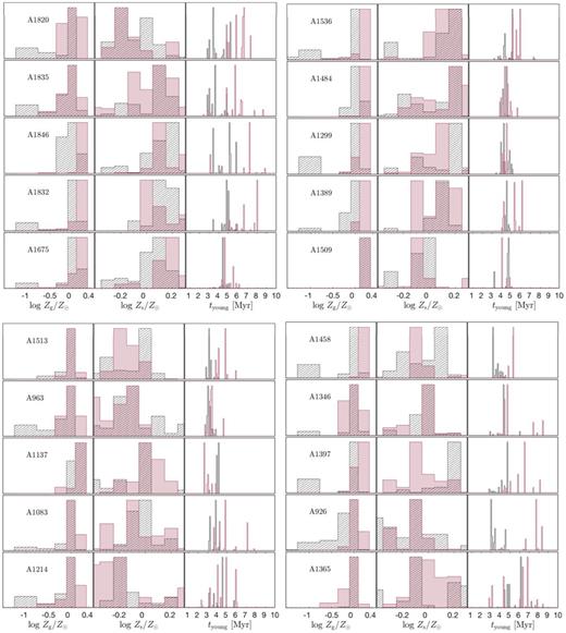
The Geneva (black dashed) versus Parsec (brown filled) fits for 20 H ii regions. The top set of panels show the PDFs of gas and stellar metallicities, and young ages (from the left- to the right-hand panels) for 10 H ii regions scattered across the western-loop. Similarly, the bottom set of panels show the PDFs for 10 regions residing in the overlap region and NGC 4039.
Certain cases, like A1137 and A1509 in Fig. B1 and A989 in Fig. 14, indicate Parsec-based light-weighted young ages predictions to be somewhat younger than the Geneva predictions. The spectra of these regions also show the blue WR bump very prominently, and in comparison, a less prominent red WR bump. In the best-fitting models shown in Fig. 14 for A989, for example, both Parsec and Geneva assign highest lightweights to a stellar population of ∼2.7 Myr in age. While Parsec predicts that an ∼2.7 Myr population solely dominates the young component of A989, Geneva also assigns some weights to an ∼3.3 and ∼4.5 Myr populations, hence biasing the estimated light-weighted young age towards a slightly older age than Parsec.
The light-weighted physical properties derived using the Geneva model library for five of the H ii regions shown in Fig. B1. The full tables containing physical properties derived using Geneva and Parsec model libraries are available online.
| Region | Young ages | |$\log \, \frac{Z_{\rm {s,1}}}{Z_{\odot }}$| | |$\log \, \frac{Z_{\rm {s,2}}}{Z_{\odot }}$| | |$\log \, \frac{Z_{\rm {g,1}}}{Z_{\odot }}$| | |$\log \, \frac{Z_{\rm {g,2}}}{Z_{\odot }}$| | |$\log \, n_{\rm {H, 1}}$| | |$\log \, n_{\rm {H, 2}}$| | log Te |
|---|---|---|---|---|---|---|---|---|
| (Myr) | (cm−3) | (cm−3) | (K) | |||||
| A1820 | 3.94 ± 1.03 | −0.1186 ± 0.1346 | −99.0 | 0.0106 ± 0.0855 | −99.0 | 2.4172 ± 0.1585 | −99.0 | 3.797 ± 0.0282 |
| A1835 | 3.57 ± 1.07 | 0.1207 ± 0.0512 | −99.0 | −0.0129 ± 0.1028 | −99.0 | 2.739 ± 0.3612 | −99.0 | 3.848 ± 0.0606 |
| A1846 | 4.77 ± 1.08 | 0.1563 ± 0.2022 | −99.0 | −0.0450 ± 0.1978 | −99.0 | 2.495 ± 0.3886 | 1.2068 ± 0.1385 | 3.805 ± 0.0634 |
| A1832 | 4.93 ± 0.40 | 0.1541 ± 0.0756 | −99.0 | 0.0256 ± 0.0935 | −99.0 | 2.3757 ± 0.1497 | −99.0 | 3.812 ± 0.037 |
| A1675 | 4.35 ± 0.41 | 0.0809 ± 0.0804 | −99.0 | 0.0379 ± 0.1096 | −99.0 | 2.5778 ± 0.2160 | 1.5905 ± 0.0851 | 3.769 ± 0.0509 |
In contrast, the Parsec and Geneva fits of, for example, A1820 and A926 in Fig. B1, point to distinctly different light-weighted young ages, where the Parsec-based age is clearly older than the Geneva-based value. In the case of A926, both Parsec and Geneva models predict the presence of an ∼3 Myr stellar population. Additionally, both Parsec and Geneva models also predict the presence of a second young population, however, at slightly discrepant ages; Parsec models predict the age to be around ∼9 Myr, and Geneva, around ∼12–13 Myr. While the ∼9 Myr versus ∼12–13 Myr is essentially a small difference, given the <10 Myr age requirement imposed in the calculation of light-weighted young ages, means that in this case, the Parsec-based light-weighted young age is biased towards older age than Geneva. Likewise, with A1820, both Parsec and Geneva models, again, predict the presence of two young stellar populations; the first around ∼3 Myr in age, and second with slightly discrepant ages with Parsec predicting an ∼7 Myr population and Geneva preferring 8−13 Myr population. This behaviour is likely primarily driven by the differences in the stellar isochrones.
The age–stellar metallicity degeneracy is also a likely reason for the differences as can be seen for A897 and A909 in Fig. B1.
Finally, there could also be some uncertainty arising from the differences in the assumed definition of solar. The solar definition of Parsec is ∼0.0169, whereas the stellar library combined with the Parsec models assume a solar value of ∼0.02. Throughout this study, we have also assumed a solar metallicity of ∼0.02.
APPENDIX C: COMPARISON WITH nH AND Te ESTIMATED FROM PYNEB
As mentioned earlier, the spectra used for this study are abundant in some of the most conspicuous emission lines in the optical, some which are widely utilized in the literature to probe the physical conditions of star-forming gas. For example, the optical diagnostics of nH include the intensity ratios of [S ii] λ6717,31Å, [Cl iii] λ5518,38Å and [Ar iv] λ4711,40Å, where each is only applicable over a specific range of densities. Likewise, the intensity ratios of [N ii] λ5755/λ6548 + 6584 and [S iii] λ6312/λ9532 + 9069 are highly sensitive to Te (Osterbrock & Ferland 2006; Peimbert et al. 2017). As the density sensitive [S ii] λ6717, 6731 Å and the temperature sensitive [N ii] λ5755, 6584 Å are relatively stronger than the others lines mentioned above, we adopt them to calculate Te and nH with aid of the publicly available PyNeb software (Luridiana et al. 2015).
The comparison between the PyNeb-based estimates of nH and Te versus those derived from fitting the Geneva and Parsec models is presented in Fig. C1. The left- and right-hand panels show the distributions of nH and Te, respectively. The nH and Te values derived from fitting the Geneva models are for the comparisons shown in the main panels, however, note that the qualitative trends are unchanged if Parsec derived values have been used instead.
![Comparison between Geneva and Parsec model predictions, and PyNeb (Luridiana et al. 2015). (a) The main panel shows the distribution of nH derived from fitting the Geneva models compared that estimated from PyNeb based on [S ii] λλ6716,31Å, with the dashed line denoting the one-to-one relation. As discussed in the text, there are cases where the best-fitting nH PDF indicate possible double solutions. For these cases, the colour-code denote the difference between the most probable and the second most probable nH values for a given spectrum. The redder colours mean the second-most likely nH is higher than the most probable value estimated from the respective PDF, and vice versa. The top panel of (a) compares the nH distributions obtained from fitting Geneva (blue) and Parsec (red) models, including the double solutions, with the distribution of PyNeb (black) estimates. (b) The distribution of light-weighted Te derived from fitting the Geneva models compared that estimated from PyNeb based on [N ii] λλ5755, 6548 Å is shown in the main panel. The dashed line, again, indicates the one-to-one relation, and the colour-code denotes the difference between the Parsec and Geneva predictions. Note that within 1σ uncertainty, the Te values obtained from Geneva and Parsec models are consistent for almost all the H ii regions, therefore the colour-code simply denote the difference between the peaks of the Gaussian fits to the Te PDFs. The top panel of (b) shows the Te distributions obtained from fitting Geneva (blue) and Parsec (red) models, and PyNeb (black) estimates.](https://oup.silverchair-cdn.com/oup/backfile/Content_public/Journal/mnras/497/3/10.1093_mnras_staa2158/1/m_staa2158figc1.jpeg?Expires=1716411860&Signature=Uk4sscDvj0Aq9mCMdNXTQ1fp6KLWSJBmRKJuXp-ZtSOsGvu9dYQFcc5SRTntnvtmLqfV26QDwrKR82HIfTORCoYJjKqRej7mG4Md9rzZfQ2peUro7XgLb7LRAzWBt-QxCNGOpmX7qP1Her5Z4G3dr8WGlx6EjcvK6UOv2v9k-vXgUCdnEPXLmoLjdZqytK~41mFjqs1vYgOYpCpXnXnpX97DvF9clZvQ5wyL-ziYIkJcU9QL0vh4FpHORZum1wfdATrEDSVgnULBlO00uoe3O~1~qrIYoen0nJBKMTZX2tXAVGcjJLJSSVnAAMmgsJ1EttqEkoxrN1xvKOD~xedcDw__&Key-Pair-Id=APKAIE5G5CRDK6RD3PGA)
Comparison between Geneva and Parsec model predictions, and PyNeb (Luridiana et al. 2015). (a) The main panel shows the distribution of nH derived from fitting the Geneva models compared that estimated from PyNeb based on [S ii] λλ6716,31Å, with the dashed line denoting the one-to-one relation. As discussed in the text, there are cases where the best-fitting nH PDF indicate possible double solutions. For these cases, the colour-code denote the difference between the most probable and the second most probable nH values for a given spectrum. The redder colours mean the second-most likely nH is higher than the most probable value estimated from the respective PDF, and vice versa. The top panel of (a) compares the nH distributions obtained from fitting Geneva (blue) and Parsec (red) models, including the double solutions, with the distribution of PyNeb (black) estimates. (b) The distribution of light-weighted Te derived from fitting the Geneva models compared that estimated from PyNeb based on [N ii] λλ5755, 6548 Å is shown in the main panel. The dashed line, again, indicates the one-to-one relation, and the colour-code denotes the difference between the Parsec and Geneva predictions. Note that within 1σ uncertainty, the Te values obtained from Geneva and Parsec models are consistent for almost all the H ii regions, therefore the colour-code simply denote the difference between the peaks of the Gaussian fits to the Te PDFs. The top panel of (b) shows the Te distributions obtained from fitting Geneva (blue) and Parsec (red) models, and PyNeb (black) estimates.
As noted in Section 3.4, we infer more than one probable nH solution for a number of H ii regions, therefore, for the comparison with PyNeb shown in Fig. C1 (left main panel), we use the most probable nH, but colour-code that to show the second nH solution. The redder (bluer) shadings indicate H ii regions with a second nH that is higher (lower) than the best-fitting nH, and the intensity of the shading denote the magnitude of the difference between the two nH values. A direct comparison between the nH distributions derived from fitting Geneva (blue) and Parsec (red) models, including all second solutions, and that calculated from PyNeb is shown in the top panel of Fig. C1.
According to the nH comparison, the majority of the model-based predictions of nH are, on average, higher than the PyNeb estimates, with a small subset of H ii regions having nH values lower than the respective PyNeb values. Those regions with a probable second nH solution also show a similar dichotomy. This is in the sense that the regions that lie above (below) the one-to-one relation have a second nH lower than their best-fit nH. The preference for the best-fitting model-based nH solutions to be biased towards higher nH values than the PyNeb solutions is further demonstrated in the top left-hand panel of Fig. C1. The Geneva distribution peaks at a somewhat higher nH than the Parsec, though there is a significant overlap between the two. In relation, the PyNeb distribution shows a peak at much lower nH. Furthermore, both Geneva and Parsec model-based nH predictions exhibit a dichotomy in their distribution, which is absent in the PyNeb distribution.
The lack of agreement between the model versus PyNeb predictions is expected given our choice of the nH diagnostic. The [S ii] doublet is largely sensitive to the low density, low-ionization zones within an H ii region, whereas, an array of low- and high-ionization emission-line ratios are used as constraints in the model fitting. Alternatively, [Cl iii] λ5518,38Å can be utilized as an indicator of the high density, central zones of an H ii region. The [Cl iii] doublet is, however, much weaker than [S ii], and resides in a part of the spectrum where the model residuals can be large.
Similarly, in the right-hand panels, we show the model- versus PyNeb-derived Te comparison. On average, we find that the model-based light-weighted Te is lower than the PyNeb estimates. This is probably due to PyNeb estimates been based on the [N ii] λ5577, 6584Å diagnostic, which likely represent a single temperature zone within an H ii region, while the model-based estimates provide an overall Te. To depict the differences between Parsec and Geneva derivations of Te, we colour-code the data points by their differences, where the bluer (redder) shadings portray the H ii regions with Geneva-based Te larger (smaller) than that of Parsec. For almost all H ii regions, the Geneva predictions of Te are larger than the Parsec values.
The top-right panel of Fig. C1 presents a Te comparison between Geneva (blue) and Parsec (red) models, and PyNeb (black), which, again, illustrate that on average PyNeb estimates of Te are larger than the model predictions. The Geneva and Parsec distributions show a substantial overlap, however, the Geneva distribution peaks at a slightly higher Te than Parsec. This behaviour of Te between the Geneva and Parsec models is expected given the tight correlation between gas metallicity and Te. Recall that Parsec, on average, yield gas metallicities that are slightly higher than Geneva, which, in turn, results in lower Te.
