Competing Reverse Channels’ Performance with Sustainable Recycle Innovation Input

Abstract

Increasing attention to sustainable development issues and recycling are forcing the recyclers to use different incentives to capture more market share. Recycling innovation input is one of the effective topics in reverse competitive chains. Because of the importance of this issue, firstly, a basic closed-loop supply chain (CLSC) system is discussed that includes an integrated manufacturer and a third-party collector. Then the impact of the integration with the innovation input into third-party product collectors is considered. Eventually, two models are constructed. The first model is a basic model that includes an integrated manufacturer and one third-party collector with innovation investment. The other model is the hybrid model that includes an integrated manufacturer and two third-party collectors with and without innovation input. Stackelberg game models are used to study the optimal pricing strategies for all three models and players’ attitudes toward different scenarios. Finally, numerical analysis is presented. Our findings are generated on the following three aspects. The collector’s recycling choice, recycling innovation input, and influence on recyclers and manufacturers. It is found that the manufacturer will always choose to recycle and prefers the hybrid recycling market, which depends on the rate of collection and the compensation from production-collecting. Moreover, the results reveal that the highest return rate of recyclers occurred under the hybrid model. However, the recyclers may not be able to invest the sustainable recycle innovation input under the exorbitant innovation barriers.

1. Introduction

In recent years, along with the trends on eco-environmental problems and sustainability, product recycling and reusing as well as sustainable development innovation have received unwavering attention of both the industrial and the academic world. Countries around the world have issued a series of policies and regulations to regulate the sustainable development of enterprises. On the one hand, the Chinese government has proposed a series of policies that combine sustainability and technological innovation. For example, in May 2016, the Ministry of Commerce and other six departments issued the Opinions on Promoting the Transformation and Upgrading of the Recycling Resources Recycling Industry, which pointed out that the main clue is to accelerate the transformation of development methods and promote the transformation and upgrading of the industry. The opinion pointed out that in line with the Internet Plus initiative development trend, the government will vigorously promote the innovation of renewable resource recovery models, and establish and perfect a renewable resource recovery system. In March 2019, the Ministry of Industry and Information Technology and the China Development Bank jointly issued the Notice on Accelerating the Promotion of Industrial Energy Conservation and Green Development, pointing out that in the qualified cities and towns, promoting the joint disposal of domestic waste by cement kilns, and promoting the comprehensive utilization of waste copper and iron, waste plastics and other renewable resources, then focusing on supporting the cascade utilization and reuse of retired new energy vehicle power batteries. Such policies, the Internet Plus, intelligent manufacturing, and online and offline integration, are designed to encourage residents and enterprises to recycle resources and promote the development of circular economy, which can not only improve resource utilization, but also protect and improve the environment. In the past, recycling channels that relied solely on physical collectors have been slowly replaced. A growing number of recycling technology companies have put forward many of their own ideas in terms of intelligent recycling, such as the Yellow Dog (the website of Yellow Dog, https://www.xhg.com), the Da Ba Shou (the website of Da Ba Shou, http://www.dabashou.com.cn), the Easy-to-Place and the Ai Hui Shou (the website of Ai Hui Shou, https://www.aihuishou.com) not only develop recycling technology, but also provide intelligent recycling equipment. This recycling equipment is often placed near people’s living environment. Compared with the traditional recycling mode, people are more willing to recycle used ones through convenient channels. At the same time, because people throw waste in smart recycling bins near their living environment, collectors can also concentrate more effectively on recycling from smart recycling bins. In general, the introduction of smart devices and 24-hour business has broken through the limitations of time and space. People can throw away waste products at a fixed point nearby at any time, which not only reduces the consumption of human resources, but also improves consumer recycling will.

On the other hand, the developed countries in the world are also actively undertaking international and social responsibilities. After the promulgation of the EU WEEE Directive, it has gradually been transformed into the legislative procedures of the EU Member States. The EU WEEE Directive 2.0 entered phase three, and the scope of control was extended to all electrical and electronic equipment. Various local governments in the United States have formulated different recycling measures, policies and regulations, such as prohibition of incineration and burial, consumers bear the cost of recycling and disposal of waste electronic and electrical products, adopt the extended production responsibility system, requiring electronic product manufacturers to bear the cost of recycling and disposal of waste electronic and electrical products, and have the responsibility to build an electronic product recycling system to collect waste of electronics and electrical products. With the efforts of the US Environmental Protection Agency, many professional electronic waste disposal companies with high and new technologies have emerged. Since 1970, the Japanese government has successively promulgated a series of laws and regulations that incorporate the concept of an extended production responsibility system, emphasizing that production enterprises must bear the major responsibility of reusing and recycling waste products, severely punishing consumer violations, actively developing a variety of recycling technologies, and constantly striving to improve the utilization ratio to used parts.

The series of similar strategies improve the external uneconomical problems of a large number of obsoleted products being discarded and accumulated, as well as the unknown environmental hazards caused by discarded electronic and electrical products lack of scientific treatment after disposal. The change in the status quo and the increase in recycling inputs greatly improve the performance of the recycling system and have a good role in promoting each entity in the closed-loop supply chain.

Manufacturers can get more low-cost recycled parts, reduce cost investment, and at the same time improve the green image in the competitive market. The green and positive manufacturer brand image can bring consumers a safer and more reliable consumer experience. The consumer viscosity is also improved. For example, all Apple’s products can be recycled. When the retailer takes the role of a recycling point, customers purchase products from the original sales channel, and then can return the used products from the original sales channel, which indirectly stabilizes the sales channel. In other words, the stability of the channel also allows consumers more trust in the brand and better recognition of the channel. From the perspective of the third-party professional recycling institutions, its introduction makes the product recycling work tend to be efficient, meticulous and professional, which can improve the efficiency of recycling. Specifically, the intelligent recycling bin can operate 24 h without labor costs, and can be automatically detected to reduce unnecessary pollution and waste. The Germany company, Reisman, specializes in the treatment of waste electronic appliances. It is mainly good at recycling waste refrigerators. It even studied and invented a set of recycling equipment for waste refrigerators. The equipment has high efficiency, advanced technology and high quality of renewable resources after treatment. However, in the past, recyclers may simply and mechanically treat, clean, dismantle, smash and so on, or discard toxic and harmful parts at will, which will bring about unknown pollution and environmental problems. In comparison, the intelligent recycling equipment has broken through the time and space restrictions. With the unified recycling and scientific treatment of professional institutions, the recycling compensation price for consumers is clearer and more transparent, but collectors charge prices that were more subjective in the past. So now, consumers will feel more reliable.

In actual life, obsolete electronic and electrical products are recycled mainly through the government’s community system, private non-profit organizations, and the voluntary collection system established by manufacturers, as well as the recent Internet Plus recycling. Then those are recycled by professional recycling technology companies and manufacturers, and are commercialized again after a series of recycling processes. For instance, packaging wastes (beer bottles), aluminum cans, etc., their reverse logistics were mainly driven by retailers, third-party collectors, and scavengers. When combined with the internet, recycling opens up a new path for low-value recyclables including low-value packaging waste, that is, the Internet Plus recycling mode, which improves consumers’ environmental awareness of recycling. Meanwhile, smart devices bring recycling convenience, price openness, and technological expertise. Therefore, the low-value recycled materials can be recycled and reused in a more concentrated, effective and economical manner.

In a simple closed-loop supply chain (CLSC), [1] showed that there are three main types of channel participants: retailers, manufacturers/remanufacturers, and third-party collectors. In fact, the industry provides a large number of examples of heterogeneous collectors with recycle innovation inputs competing. For example, Shandong Zhonglv is a third-party recycling enterprise specializing in recycling and disposal of waste electrical and electronic products. With its leading domestic processing scale and technology, it provides professional recycling, dismantling, and inspection services for Hisense’s old home appliance recycling. While the rise of third-party recycling companies, such as Hangzhou Dadi Environmental Protection Co., Ltd. and Shenyang Muchang International Environmental Protection Industry, will inevitably lead to competition among third-party collectors. At the same time, there are a large number of small collectors in the market that purchase eliminated electronic and electrical products from consumers, and then the integrated manufacturers buy second-hand raw materials or retired products from the competing collectors. Obviously, on the one hand, investing a certain amount of innovative inputs in recycling will increase the amount of recycling. For example, Shandong Zhonglv’s more professional recycling technology and recycling services have improved the profitability of product recycling. Another example, the innovative recycling model of Ai Hui Shou improves the convenience of recycling and consumers’ awareness of recycling simultaneously. Therefore, for high-quality recycling of electronic products, consumers can obtain considerable recycling rewards in recycling transactions, and they will be more willing to accelerate the replacement of electronic products, which indirectly drives the demand for emerging electronic products. On the other hand, competition between heterogeneous collectors will have a substantial impact on the efficiency of recovery of the entire CLSC and even performance. Just as more and more environmental protection companies and recycling companies are playing the role of third-party collectors in the market, considering the competition of third-party collectors with or without innovative investment, it is more suitable for the actual situation.

In this study, we firstly discuss a basic CLSC system that includes an integrated manufacturer and a third-party collector. Reference [2] paid particular attention to the role of technological innovation as evidenced through patent activities in the waste recovery sector. Whether spontaneously through the market or as a consequence of policy interventions, technological innovation can play a significant role in overcoming failures in recycling markets. Thus, on the basis of the basic supply chain system, we consider the impact of the innovation input, and we construct the two models, one of the models includes an integrated manufacturer and a third-party collector with innovation investment, another model is the hybrid model that includes an integrated manufacturer and two third-party collectors with and without innovation input.

Based on the above model, we aim to solve the following research problems:

1.

How the recycling innovation inputs affect the retail price, transfer price, collection effort, supply chain agents’ decisions and performance?

2.

How does horizontal competition among recyclers affect the optimal strategy and optimal channel performance of closed-loop supply chain node enterprises?

The remainder of the paper is organized as follows. In Section 2, we provide a literature review with three aspects, namely closed-loop supply chains with remanufacturing, competition in remanufacturing, innovation input incentives in remanufacturing a closed-loop supply chain. In Section 3, we define the model parameter and then introduce the basic research problem, and related model assumptions. In Section 4, we propose a basic closed-loop supply chain model and a hybrid closed-loop supply chain system that includes innovative inputs. Section 5 gives the analysis results. We conclude and outline the limitations of this work and possible directions for future research in Section 6. The proofs of the theorems, lemmas and propositions can be found in the Appendix A.

2. Literature Review

In this section, we present a review of the related literature on three research fields, i.e., closed-loop supply chains with remanufacturing, competition in remanufacturing, and innovation input incentives in remanufacturing closed-loop supply chain.

2.1. Closed-Loop Supply Chains with Remanufacturing

First, this paper is most closely related to the CLSC system with remanufacturing. In this area, Reference [1] considered a manufacturer-led CLSC in a Stackelberg game, which has three options for product collection activities and found that the retailer is the most effective undertaker. Moreover, Reference [3] extended the two-stage supply chain collection model as explored in many of the above-reviewed studies to a three-tier supply chain coordination problem under different channel leadership. Since then, many scholars have compared these three single channels in pairs; for example, [4,5,6]. However, their works only focus on one period problem. Reference [7] presented a two-period closed-loop green supply chain model with a single manufacturer and a single retailer to investigate the impact of green innovation, marketing effort and collection rate of used products on the supply chain decisions. Some scholars proposed a dual distribution channel consisting of traditional retail channels and e-tail (internet) ([5,6,8]), a dual recovery channel hybrid manufacturing-remanufacturing production model [9], but the above researches focused on the collecting channels of the third-party collectors is less. In recent years, with the rise of online recycling service platforms, third-party collection channels have attracted more and more attention from scholars. For example, the authors of [5] dealt with a closed-loop supply chain with two dual channels—a forward dual-channel where a manufacturer sells a product to customers through traditional retail channel and e-tail (internet) channels, and a reverse dual-channel where the used items are collected for remanufacturing through the traditional third party logistics and e-tail channel. Reference [10] considered consumers might choose the online collection service provided by third-party platforms for convenience and explore the influence of consumer behavior on the competitive dual-collecting supply chain. With the spread of digitalization, a virtual logistics company plays a very important role, not only in a regular supply chain, but also in some emerging supply chain areas. For instance, Reference [11] study an implementation of a virtual logistics network for PCs with remanufacturing and [12] investigate the possibilities of establishing and operating virtual logistics centers in a cross-border logistics area.

2.2. Competition in Remanufacturing

Second, the authors of [13] extended the study of [1] to a setting where two retailers compete in the forward supply chain, and studied the coordination problem in the indirect collection model. Subsequently, many scholars ignited fierce discussions about the competition between closed-loop supply chain recycling channels and the choice of recycling channels. On the basis of a single recycling channel, the authors of [14] discussed the recycling model of retailers and third-party companies, and found that the prices of remanufactured products under the recycling channels of third-party companies were higher than the prices of products recovered by retailers. In comparison, the recycling channels of third-party companies are most affected by the marginal effect. Reference [15] considered that the retailer collects used products with a third-party and remanufactures used products at the same time. Reference [16] studied a supply chain in which the collecting of waste products is by the manufacturer and the third-party, and three individuals are leaders of a Stackelberg game. Reference [17] proposed a dual-recycling situation where retailers and third parties compete with each other. Research showed that when recycling competition is fierce, dual-recycling channels are superior to traditional single-recycling channels. On the basis of dual recycling channels, the authors of [18] set up two dual-collecting channel models: one that is the collecting of waste products by the manufacturer and the retailer, and another that is the collecting of waste products by the manufacturer and the third-party. Then, the authors of [19] found dual-collecting competition has significant influence on the supply chain. Reference [20] studied the two chains compete with each other in three competition structures: the Centralized Competition Game, the Hybrid Competition Game (including two cases), and the Decentralized Competition Game. Reference [21] studied the influence of collecting convenience on collecting rate in a dual collecting model. Reference [22] considered two collecting reverse supply chains consisting of a retailer and a manufacturer, who compete together by proposing more rewards to the customers. Competition between two channels of one chain infers to internal competition, and external competition that points out to competition among two supply chains.

With the rapid development of smart logistics, the recycling model of waste products has gradually shifted to the Internet Plus recycling, and the way of third-party recycling occupies an increasingly important position. Reference [10] considered consumers might choose the online collection service provided by third-party platforms for convenience, which also brings competition to other channels. To explore the influence of consumer behavior on the competitive dual-collecting supply chain. Reference [23] considered a closed-loop supply chain (CLSC) with a competitive recycling-market (competitive collectors) and product-market (new and remanufactured products). According to the above literature, such as [1,3], the third-party recycler is the most unfavorable recycling method, but with the support of the internet, the third-party recycler’s innovative investment in recycling work has greatly overcome the disadvantages of third-party recycling, not only in the external impact. It has increased consumer demand and improved recycling efficiency, and realized the unrealized value of waste products from recycled products [24]. Those problems we proposed above are also the research questions we would like to discuss in this particular study.

2.3. Innovation Input Incentives in Remanufacturing Closed-Loop Supply Chain

Finally, we discussed relevant literature on innovation inputs. Reference [25] mainly studied how the competition between the two reverse channels influence supply chain players’ optimal decisions and channel performance. In their work, however, they ignored the impact of the innovation input. Reference [26] examined the development and current state of supply chain innovation research in management and identified research gaps. Reference [2] emphasized imperfect and asymmetric information and technological and consumption externalities such failures that can be overcome (in part) by technological innovation. For example, the authors of [27] reported a simple, effective and sustainable method for the recovery of precious metals from end-of-life vehicle shredder residue and/or automobile shredder residue based on a hybrid ball-milling and microbubble froth flotation process. The authors of [28] used an innovative disassembly approach to identify the profitability of recycling such electronic components. Reference [29] also showed that the retailer remanufacturing after paying for the fixed technology authorization fees remanufacturing (FR) mode not only promotes the retailer to improve the product service level, but also enables the third-party to improve the recovery rate. Reference [9] first identified the root causes of the low return rate of cell phones and then developed a novel Radio Frequency Identification (RFID) based return channel to increase the recycling rate. A mathematical model is developed considering the cost of implementation and the design of the proposed RFID based recovery channel. Reference [30] contributed on waste product collection and remanufacturing by taking the intellectual property rights of the original manufacturer into consideration. Reference [31] found that during the pretreatment process, the failure to operate on high-value materials caused significant economic losses (from 2006 to 2014, computer and mobile phone losses exceeded 70 million dollars). This is also the necessity of this article to explore innovative investment in recycling channels. We have also found that in many documents, specific innovative technologies and innovative models are introduced into the recycling and remanufacturing process. Reference [32] provided an overview of the status of the waste electrical and electronic equipment (WEEE) collection system in China, combined the brick-and-mortar and the internet, and generated four WEEE collection systems. Moreover, the authors of [33] analyzed the effect of environmental subsidies on the incentives of investing in emission-reducing technologies in manufacturing amid the environmental concerns of consumers. Reference [8] said the performance of the supply chain can be improved by instigating either green innovation or marketing effort or both. For example, the authors of [34] focused on the impact of competition and consumers environmental awareness on key supply chain players. Also, they found that as consumers environmental awareness increases, retailers and manufacturers with superior eco-friendly operations will benefit. In addition, many emerging countries are also involved with their corresponding innovation management in their manufacturing industries. For instance, the authors of [35] use Data Envelopment Analysis to investigate the effectiveness of invested finances in the innovation of small- and medium-sized production enterprises in Slovakia. Furthermore, in [36], the authors developed a bibliometric analysis to investigate how the innovation factors benefit to a strategic manager with their given innovative activities.

3. Problem Description and Assumption

3.1. Problem Description

In this section, we firstly discuss a basic closed-loop supply chain system that includes an integrated manufacturer and a third-party collector. Secondly, we consider the impact of the innovation input, and we construct the two models. One of the models includes an integrated manufacturer and a third-party collector with innovation investment. The other model is the hybrid model that includes an integrated manufacturer and two third-party collectors with and without innovation input. The integrated manufacturer produces the new product and sells it to the consumer directly. We assume that the manufacturer only recycles from third-party recycling channels to implement remanufacturing. The collector recycles from the market directly and sells the used products to the manufacturer. The two or three parties will all pursue optimal profit by making their decision or effort strategies under Stackelberg games. For example, Ai Hui Shou implement smart recycling bins in residential areas, schools, commercial squares and other places. Due to the popularity of smart phones and the background of the intelligent community, people are more likely to put used products into smart recycling bins and get certain variable remuneration. In the model, the manufacturer allocates the reverse channel responsibility to the collectors, and products are collected indirectly via the collectors. The CLSC structures under different business models are as follows.

3.2. Assumption

In this reverse channel model, collected used products are transferred to the manufacturer by the collectors in return of a fixed per-unit buy-back payment, $b_i$. Subscript i takes the values of 1 and 2, denoting the collector 1 and collector 2, respectively. Given the retail price p and the buy-back payment $b_1$ and $b_2$, each collector $i(i=1,2)$ solves for the optimal innovation input e and the collection effort ${\tau }_i$, taking into consideration the competition from the other collectors. The manufacturer chooses the retail price p and the buy-back price b, taking into consideration the effect of these decisions on the strategic decisions of the collectors. Consistent with the extant literature ([7,8]), we assume that in that model, the manufacturer has sufficient channel power over the collectors to act as a Stackelberg leader, and the collectors compete in a Bertrand pricing game. We characterize the supply chain performance for each model in terms of the pricing decisions of the manufacturer and collectors, the collection effort, total supply chain profits, and the allocation of total profits between the manufacturer and the collectors.

In the rest of the paper, the following notation is used: $c_m$ denotes the unit cost of manufacturing a new product, and $c_r$ the unit cost of remanufacturing a returned product into a new one. ${\Pi }_j$ denotes the profit function for channel member j. Subscript j takes the values of M, C, $C_1$, and $C_2$, denoting the manufacturer, the collector, the collector 1, and collector 2, respectively. While the manufacturer takes back the used product from collector i at a price $b_i(i=1,2)$. $D(p,e)$ denotes the demand at market as a function of the selling price p and collector’s innovation input e. R denotes cost coefficient of recycling innovation input. Due to the vertical externality brought by the recycling innovation input, we assume that e plays a positive role in the demand of consumers. We denote the returned quantity as $\tau D(p,e)$, and $0<\tau <1$, where $\tau$ represents the reverse channel performance and it is a function of the product collection effort. $\tau$ also denotes the fraction of the current generation products remanufactured from the returned units [13]. We assume the market demand function as a deterministic linear function of the retail price p and the innovation input e.

$$\begin{array}{c}\hfill D(p,e)=\alpha -\beta p+Ke\end{array}$$

(1)

where $\alpha >0$, $\beta >0$, the constant $\alpha$ indicates the market potential while the coefficient $\beta$ represents the sensitivity of demand to price changes. $K>0$, and K represents the demand expansion effectiveness coefficient of the innovation input by the collector, also the coefficient K measures the marginal consumer demand with respect to the innovation input e. When $\beta \ge K$, it means that consumers are more sensitive to the sales price of the product than the innovative input coefficient provided by the collector. When $\beta <K$, it is contrary to the above statement. p represents the retail price of the unit determined by the manufacturer, and e represents the recycling innovation investment of the collector. $\alpha >\beta p$, that is, this is a rational market, and reasonable pricing controls the basis of the general market. This form of demand function has been adapted separately by the research community ([34,37,38]).

The average unit cost of manufacturing can hence be written as $c=c_m(1-{\tau }_i)+c_r{\tau }_i$ (c.f., [3,13]). We assume that $\alpha -\beta c_m>0$. The reverse channel performance is characterized by $\tau$, the return rate of used products from the customers. $\tau$ denotes the fraction of the current generation of products supplied from returned and thus remanufactured units, i.e., $0<\tau <1$. e denotes innovation input of collection activities by collectors which can be understood as not only the investment in the recycling technology (disassembly, refining, etc., and the technology of the intelligent recycling machine), but also the innovation in the recycling mode (the release of the intelligent recycling machine). There are now more than a dozen large-scale waste product recycling platforms, such as Ai Hui Shou, Hui Shou Bao (the website of Hui Shou Bao, https://www.huishoubao.com) and other Internet Plus recycling platforms. Compared with the recycling mode of a petty dealer, it breaks the space limitation and improves the enthusiasm of consumers to participate. People are more willing to recycle used products to recyclers in exchange for a certain variable return. For example, Ai Hui Shou gives different rewards to customers regarding the quality rating for their electronic products. The better the product, the higher the reward. Therefore, the investment in recycling innovation will also stimulate consumer demand for new products to a certain extent. By focusing only on promotional and innovation’s expenses to collect used products, we control for the strategic consumer behavior and solely focus on the channel behavior of the manufacturer and the collectors. Hence, consumers in our model react only to new product prices and innovation input.

The total cost of collection $C\left(\tau \right)$ can be characterized as a function of returned rate and unit innovation input of used products and is given by

$$\begin{array}{c}\hfill C({\tau }_i,e)=\frac{H}{2}{\tau }_i^2+\frac{R}{2}{e}^2+A{\tau }_{i}D(p,e)\end{array}$$

(2)

where A denotes the variable unit cost of collecting and handling a returned unit (e.g., a fixed payment given to the consumer who returns a used product). For simplicity of calculation, we set A as a constant. H and R are scaling parameters, and $H,R>0$. Notice that in order to characterize the diminishing return of investment with respect to ${\tau }_i$ and e, we use the quadratic cost structure. To ensure that the remanufacturing process is economically viable, we have $A<c_m-c_r$, $A<b$.

Several papers in the operations management literature, such as [22,25], addressed cost structure problems taking into consideration the effects on the self-reward of each channel and cross-rewards that are suggested to the customer by the competitors in the other channels.

In summary, the following assumptions are made for the model in this paper,

Assumption A1.

All supply chain members are rational with the aim of maximizing profits.

Assumption A2.

We assume that all supply chain members have access to the same information while optimizing their objective functions.

Assumption A3.

In the basic closed-loop supply chain system which does not consider the recycling innovation inputs, the following assumption is established: $4H-\beta {(\Delta -A)}^2>0$.

Assumption A4.

In the basic closed-loop supply chain system which considers the recycling innovation inputs, the following assumptions are established: $\beta R-K^2>0$, $RH-\frac{K^2{\beta }^2{R}^2{(\Delta -A)}^2}{4{(\beta R-K^2)}^2}$ and $RH-\frac{{\beta }^2{R}^2{(\Delta -A)}^2}{4(\beta R-K^2)}>0$.

Assumption A5.

In the hybrid closed-loop supply chain system which considers the recycling innovation inputs, the following assumptions are established: $\beta R-K^2>0$, $RH-\frac{K^2{\beta }^2{R}^2{(\Delta -A)}^2}{4{(\beta R-K^2)}^2}$ and $RH-\frac{\beta R(2\beta R-K^2){(\Delta -A)}^2}{4(\beta R-K^2)}>0$.

4. Model Formulation and Solution

In the real practice, we explore that their optimal retailing price, transfer price and collection effort may have some special influences on their performance. Therefore, we generate this model to explore their decision variables, that is, retail price p and transfer price b by the manufacturer, collection effort $\tau$ and innovation input e by the collector. Without loss of generality, we generate the manufacturing and the direct selling by an integrated manufacturer who produces products with remanufactured components and new components, and sell it to the end customers with selling price p in the system.

4.1. Basic System without Innovation Input (Model B)

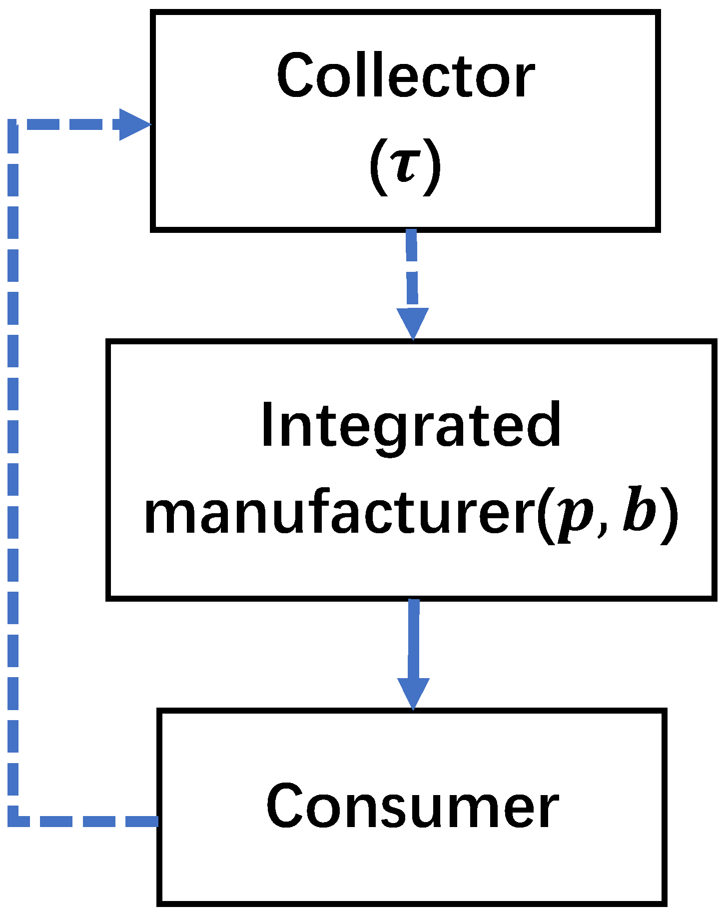
Now, we start with the simple supply chain described above, including one collector and one manufacturer. Figure 1 shows this basic supply chain system structure. As the basic model, we first study the vertically integrated manufacturer that directly sells its product to consumers and one collector without innovation input e.

The demand function of the basic system without innovation input (model B) is given as:

$$\begin{array}{c}\hfill D^B\left(p\right)=\alpha -\beta p\end{array}$$

(3)

Many manufacturers play as leaders in the respective supply chains. They have strong market power to influence the decisions of other supply chain participants. As such, we consider that the integrated manufacturer has the power to determine the retail price and the transfer price. At first, the manufacturer determines the transfer price b and the selling price p. Afterward, the collector determines the return rate of used product $\tau$.

The profit function of the collector of the basic model (model B), ${\Pi }_C^B$ (the superscript B representing basic model without innovation input e and the subscript C representing the collector), is as follows,

$$\begin{array}{c}\hfill {\Pi }_C^B\left(\tau \right)=b\tau D\left(p\right)-A\tau D\left(p\right)-\frac{H}{2}{\tau }^2\end{array}$$

(4)

Solving the stage two optimization problem first, the collector’s response function can be obtained as,

$$\begin{array}{c}\hfill \tau (p,b)=\frac{(b-A)(\alpha -\beta p)}{H}\end{array}$$

(5)

Further, the profit function of the manufacturer (denoted with a subscript M ) of model B is as follows,

$$\begin{array}{cc}\hfill {\Pi }_M^B(p,b)& =[p-c_m+(c_m-c_r-b\left)\tau \right]D^B\left(p\right)\hfill \\ \hfill & =[p-c_m+(\Delta -b\left)\tau \right]D^B\left(p\right)\hfill \end{array}$$

(6)

where $\Delta =c_m-c_r$.

The following proposition describes the findings in the basic model without innovation input e.

Theorem 1.

To solve the manufacturer’s problem, we substitute the obtained response function (5) into the manufacturer’s profit function (6) and jointly optimize over the manufacturer’s decisions (p, b). It can be obtained that $b^{B*}=\frac{\Delta +A}{2}$, and $p^{B*}=\frac{\alpha +\beta c_m-2\alpha \beta \frac{{(\Delta -A)}^2}{4H}}{2\beta -2\beta \left(\beta \right)\frac{{(\Delta -A)}^2}{4H}}$. Based on the optimal decisions, the collector’s collection effort τ can also be obtained as, ${\tau }^{B*}=\frac{(\Delta -A)(\alpha -\beta c_m)}{4H-\beta {(\Delta -A)}^2}$. The optimal profits can be obtained as, ${\Pi }_M^B(p,b)=\frac{H{(\alpha -\beta c_m)}^2}{\beta [4H-\beta {(\Delta -A)}^2]}$, ${\Pi }_C^B\left(\tau \right)=\frac{H}{2}{\left[\frac{(\Delta -A)(\alpha -\beta c_m)}{4H-\beta {(\Delta -A)}^2}\right]}^2$, and ${\Pi }_c^B\left(\tau \right)+{\Pi }_M^B(p,b)=\frac{H{(\alpha -\beta c_m)}^2[8H-\beta {(\Delta -A)}^2]}{2\beta {[4H-\beta {(\Delta -A)}^2]}^2}$.

Lemma 1.

If the condition of $H>\frac{\beta {(\Delta -A)}^2+(\Delta -A)(\alpha -\beta c_m)}{4}$ is satisfied, then ${\tau }^{B*}=\frac{(\Delta -A)(\alpha -\beta c_m)}{4H-\beta {(\Delta -A)}^2}$ is between 0 and 1.

From the above analysis, it can be seen that the cost coefficient of recycling efforts H has a minimum value. Below the minimum value does not meet the actual situation, nor does it conform to the assumptions of this article. In other words, if the recycling cost factor H of recycling efforts is small, that is to say, the difficulty of recycling is small and the recycling rate may exceed 1. It is also reflected from the negative side that the recycling cost in real life is high and the recycling difficulty is great. On the other hand, as the transfer price rises, it will indirectly increase the difficulty of recovery.

4.2. Basic System with Innovation Input (Model BE)

Next, in Figure 2, we consider a similar basic supply chain structure consisting of a manufacturer and a collector, in which the collector invests in innovation input in the process of collection. As mentioned in the above assumptions, the demand function of the market can be expressed as, $D^{BE}(p,e)=\alpha -\beta p+Ke$.

The collector’s profit function of the model $BE$ can be written as,

$$\begin{array}{c}\hfill {\Pi }_C^{BE}\left(\tau ,e\right)=b\tau D^{BE}(p,e)-A\tau D^{BE}(p,e)-\frac{H}{2}{\tau }^2-\frac{R}{2}{e}^2\end{array}$$

(7)

From the concavity of the objective functions, the best response functions are determined by the simultaneous solution of first-order conditions for ${\tau }^{BE}$, $e^{BE}$.

The optimal product return rate is ${\tau }^{BE}(b,p)=\frac{R(b-A)(\alpha -\beta p)}{RH-K^2{(b-A)}^2}$. The optimal innovation input is $e^{BE}(b,p)=\frac{K{\left(b-A\right)}^2(\alpha -\beta p)}{RH-K^2{\left(b-A\right)}^2}$.

The manufacturer’s profit function can be written as,

$$\begin{array}{c}\hfill {\pi }_M^{BE}(p,b)=(p-c_m+(c_m-c_r-b\tau )D^{BE}(p,e)\end{array}$$

(8)

Theorem 2.

We substitute the obtained the closed-form solutions of ${\tau }^{BE}$ and $e^{BE}$ into the manufacturer’s profit function (8) and jointly optimize over the manufacturer’s decisions (p, b).

$$\begin{array}{cc}\hfill b^{BE*}=& \frac{\beta R(\Delta +A)-2K^{2}A}{2\beta R-2K^2}\hfill \end{array}$$

(9)

$$\begin{array}{cc}\hfill p^{BE*}=& \frac{\left(\alpha +\beta c_m\right)M-2\alpha \beta RN}{2\beta M-2{\beta }^{2}RN}\hfill \end{array}$$

(10)

where $M=RH-\frac{K^2{\beta }^2{R}^2{(\Delta -A)}^2}{4{\left(\beta R-K^2\right)}^2}$, $N=\frac{\beta R\left(\beta R-2K^2\right){(\Delta -A)}^2}{4{\left(\beta R-K^2\right)}^2}$.

Substituting $b^{BE*}$, $p^{BE*}$ into the collector’s profit function, then the optimal decisions are given as follows,

$$\begin{array}{cc}\hfill {\tau }^{BE*}=& \frac{\beta R}{\beta R-K^2}*\frac{R(\Delta -A)\left(\alpha -\beta c_m\right)}{4M-4\beta RN}\hfill \end{array}$$

(11)

$$\begin{array}{cc}\hfill e^{BE*}=& \frac{K}{2}\frac{{\left[\beta R\right]}^2}{{\left[\beta R-K^2\right]}^2}\frac{{(\Delta -A)}^2\left(\alpha -\beta c_m\right)}{4M-4\beta RN}\hfill \end{array}$$

(12)

Thus, the optimal profit functions can be obtained as,

$$\begin{array}{cc}\hfill {\Pi }_M^{BE*}(p,b)=& \frac{RH{\left(\alpha -\beta c_m\right)}^2}{\beta (4M-4\beta RN)}\hfill \\ \hfill {\Pi }_C^{BE*}(p,b)=& \left[\frac{H}{2}-\frac{R}{8}{\left(\frac{\beta K(\Delta -A)}{\left(\beta R-K^2\right)}\right)}^2\right]{\left[\frac{R*\beta R(\Delta -A)}{\beta R-K^2}*\frac{\left(\alpha -\beta c_m\right)}{4M-4\beta RN}\right]}^2\hfill \\ \hfill {\Pi }_T^{BE*}(p,b)=& \frac{RH{\left(\alpha -\beta c_m\right)}^2}{\beta (4M-4\beta RN)}+\left[\frac{H}{2}-\frac{R}{8}{\left(\frac{\beta K(\Delta -A)}{\left(\beta R-K^2\right)}\right)}^2\right]{\left[\frac{R*\beta R(\Delta -A)}{\beta R-K^2}*\frac{\left(\alpha -\beta c_m\right)}{4M-4\beta RN}\right]}^2\hfill \end{array}$$

Lemma 2.

If the condition of $H>\frac{\beta {(\Delta -A)}^2}{4\left(\beta R-K^2\right)}\left[\frac{R\left(\alpha -\beta c_m\right)}{(\Delta -A)}+\beta R\right]$ is satisfied, then ${\tau }^{BE*}=\frac{\beta R}{\beta R-K^2}*\frac{R(\Delta -A)\left(\alpha -\beta c_m\right)}{4M-4\beta RN}$ is between 0 and 1.

From the above analysis, after the integration of innovative investment, it can be seen that the threshold of the cost coefficient of recycling efforts H has increased compared with that in the basic model B. In other words, when recyclers invest on the innovation, they also increase the entry barriers to the innovational recycling.

Lemma 3.

When $\Delta >b$, we can get $R>\frac{2K^2}{\beta }$. In this case, it means that the threshold of the recycling innovation cost coefficient is raised, that is, the barriers to recycling innovation are raised. Under the current conditions, with the increase of b, it also indirectly improves the difficulty of recycling efforts. Such situations are more in line with the actual situation.

4.3. Hybrid System (Model H)

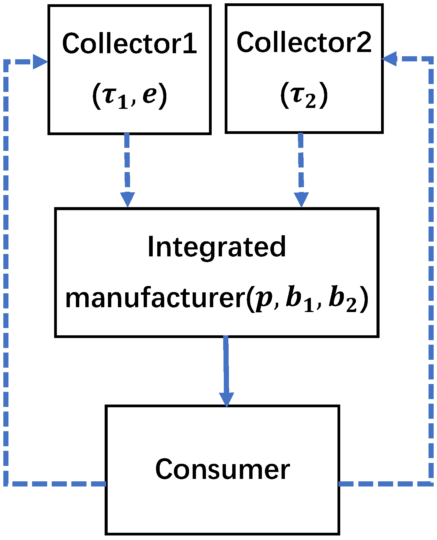
In the hybrid system, there is an integrated manufacturer and two collectors. The structure of the game played between the manufacturer and the collectors in the reverse channels is as follows. In this reverse channel model, collectors engage only in the recovering of the product while the integrated manufacturer participates in both manufacturing and distribution. The integrated manufacturer decides on the retail price of the product p, transfer price $b_1$ (per unit returned) reimbursed to the collector 1 and transfer price $b_2$ (per unit returned) reimbursed to the collector 2. We consider that one of the collectors with innovation input (collector 1) decides on the investment in product collection effort ${\tau }_1$ as well as the innovation input e of the recycling process. While the other one without innovation input (collector 2) determines the product collection effort ${\tau }_2$ by taking into account the retail price charged by the manufacturer and the competition from the other collector 1 with innovation input. Both collectors reimburse each consumer a fixed fee A, per unit returned. We assume that in the model, the manufacturer has sufficient channel power over the retailers to act as a Stackelberg leader, and the collectors compete in a Bertrand pricing game. Figure 3 shows this hybrid supply chain system structure.

When obsoleted products are returned to the collectors directly, the manufacturer has strong market power to influence the decisions of other supply chain members, so he firstly determines the transfer price $b_i(i=1,2)$, the subscript 1, 2 represents collector 1 and collector 2, and the selling price p. Secondly, the collectors determine the optimal return rates of used product ${\tau }_1$, ${\tau }_2$ and the optimal innovation input e. For example, the recycling mode of electronic equipment products such as mobile phones is similar to the recycling mode described above. Mobile phones can be recycled from the recycling channels of professional recyclers, from smart recycling bins, and from petty dealers.

The profit function of the collector 1 with innovation input e in the model H is ${\Pi }_{C_1}^H$(the superscript H representing the hybrid system and the subscript $C_1$ representing the collector 1).

Given p and $b_1$, the collector 1 solves the following profit function to determine the investment in product collection effort and the innovation input.

$$\begin{array}{c}\hfill {\Pi }_{C_1}^H\left({\tau }_1,e\right)=b_1{\tau }_{1}D-A{\tau }_{1}D-\frac{H}{2}{\tau }_1^2-\frac{R}{2}{e}^2\end{array}$$

(13)

From the concavity of the objective functions, the best response functions are determined by the simultaneous solution of first-order conditions for ${\tau }_1^H$, $e^H$.

The optimal product return rate is ${\tau }_1^H\left(b_1,p\right)=\frac{R\left(b_1-A\right)(\alpha -\beta p)}{RH-K^2{\left(b_1-A\right)}^2}$. The optimal innovation input is $e^H\left(b_1,p\right)=\frac{K{\left(b_1-A\right)}^2(\alpha -\beta p)}{RH-K^2{\left(b_1-A\right)}^2}$.

Hence the collector 2 without innovation input optimizes the following problem (the subscript $C_2$ representing the collector 2).

$$\begin{array}{c}\hfill {\Pi }_{C_2}^H\left({\tau }_2\right)=b_2{\tau }_{2}D-A{\tau }_{2}D-\frac{H}{2}{\tau }_2^2\end{array}$$

(14)

From the concavity of the objective function, we can easily show that, ${\tau }_2^H\left(b_1,b_2,p\right)=\frac{R\left(b_2-A\right)(\alpha -\beta p)}{RH-K^2{\left(b_1-A\right)}^2}$.

Furthermore, the manufacturer’s profit function is given below,

$$\begin{array}{c}\hfill {\Pi }_M^H(p,b_1,b_2)=(p-c_m)D(p,e)+(c_m-c_r-b_1){\tau }_{1}D(p,e)+(c_m-c_r-b_2){\tau }_{2}D(p,e)\end{array}$$

(15)

Theorem 3.

When the parameters satisfy $H>\frac{\beta {(\Delta -A)}^2}{4}*\frac{2\beta R-K^2}{\beta R-K^2}$, $\beta R-K^2>0$. The manufacturer’s profit function is concave and has a unique maximum value.

It is straight forward to find that the optimal solutions for the manufacturer’s profit function are

$$\begin{array}{cc}{b}_1^{H*}=\hfill & \frac{\beta R(\Delta +A)-2K^{2}A}{2\beta R-2K^2}\hfill \end{array}$$

(16)

$$\begin{array}{cc}{b}_2^{H*}=\hfill & \frac{\Delta +A}{2}\hfill \end{array}$$

(17)

$$\begin{array}{cc}{p}^{H*}=\hfill & \frac{\left(\alpha +\beta c_m\right)M-2\alpha \beta RN-\frac{{(\Delta -A)}^2}{2}\alpha \beta R}{2\beta M-2{\beta }^{2}RN-\frac{{(\Delta -A)}^2}{2}{\beta }^{2}R}\hfill \end{array}$$

(18)

where $M=RH-\frac{K^2{\beta }^2{R}^2{(\Delta -A)}^2}{4{\left(\beta R-K^2\right)}^2}$, $N=\frac{\beta R\left(\beta R-2K^2\right){(\Delta -A)}^2}{4{\left(\beta R-K^2\right)}^2}$.

$b_2$ is independent of p, $b_1$, while p and $b_1$ affect each other. With the above analytical results, we can derive Theorem 4.

Theorem 4.

$H>0$, $R>0$, $RH-\frac{K^2{\beta }^2{R}^2{(\Delta -A)}^2}{4{\left(\beta R-K^2\right)}^2}>0$ are satisfied, the optimal decisions of collectors are given as follows.

$$\begin{array}{cc}\hfill {\tau }_1^{H*}=& \frac{\beta R}{\beta R-K^2}*\frac{R(\Delta -A)\left(\alpha -\beta c_m\right)}{4M-4\beta RN-\beta R{(\Delta -A)}^2}\hfill \end{array}$$

(19)

$$\begin{array}{cc}\hfill {\tau }_2^{H*}=& \frac{R(\Delta -A)\left(\alpha -\beta c_m\right)}{4M-4\beta RN-\beta R{(\Delta -A)}^2}\hfill \end{array}$$

(20)

$$\begin{array}{cc}\hfill e^{H*}=& \frac{K}{2}\frac{{\left[\beta R\right]}^2}{{\left[\beta R-K^2\right]}^2}\frac{{(\Delta -A)}^2\left(\alpha -\beta c_m\right)}{4M-4\beta RN-\beta R{(\Delta -A)}^2}\hfill \end{array}$$

(21)

where $M=RH-\frac{K^2{\beta }^2{R}^2{(\Delta -A)}^2}{4{\left(\beta R-K^2\right)}^2}$, $N=\frac{\beta R\left(\beta R-2K^2\right){(\Delta -A)}^2}{4{\left(\beta R-K^2\right)}^2}$.

Theorem 5.

The optimal profit functions can be obtained as,

$$\begin{array}{cc}\hfill {\Pi }_M^{H*}=& \frac{RH{\left(\alpha -\beta c_m\right)}^2}{\left[4M-4\beta RN-\beta R{(\Delta -A)}^2\right]\beta }\hfill \end{array}$$

(22)

$$\begin{array}{cc}\hfill {\Pi }_{c_1}^{H*}\left({\tau }_1,e\right)=& \left[\frac{H}{2}-\frac{R}{8}{\left(\frac{\beta K(\Delta -A)}{\left(\beta R-K^2\right)}\right)}^2\right]{\left(\frac{\beta R}{\beta R-K^2}*\frac{R(\Delta -A)\left(\alpha -\beta c_m\right)}{4M-4\beta RN-\beta R{(\Delta -A)}^2}\right)}^2\hfill \end{array}$$

(23)

$$\begin{array}{cc}\hfill {\Pi }_{c_2}^{H*}\left({\tau }_2\right)=& \frac{H}{2}{\left[\frac{R(\Delta -A)\left(\alpha -\beta c_m\right)}{4M-4\beta RN-\beta R{(\Delta -A)}^2}\right]}^2\hfill \end{array}$$

(24)

where $M=RH-\frac{K^2{\beta }^2{R}^2{(\Delta -A)}^2}{4{\left(\beta R-K^2\right)}^2}$, $N=\frac{\beta R\left(\beta R-2K^2\right){(\Delta -A)}^2}{4{\left(\beta R-K^2\right)}^2}$.

Lemma 4.

If the condition of $H>\frac{\beta {(\Delta -A)}^2}{4\left(\beta R-K^2\right)}\left(\frac{\left(\alpha -\beta c_m\right)\left(2\beta R-K^2\right)}{\beta (\Delta -A)}+2\beta R-K^2\right)$ is satisfied, then ${\tau }_1^{H*}$, ${\tau }_2^{H*}$, ${\tau }_1^{H*}+{\tau }_2^{H*}$ are all between 0 and 1.

Compared with the previous two models, the cost coefficient of the collection effort H has the highest threshold in model H, that is to say, the system has the highest difficulty. The hybrid system is also much more close to real life, which also reflects the high recycling cost and the difficulty of recycling in real life.

Lemma 5.

In some cases, $b_1^{H*}>\Delta$ will appear. In this case, although it will greatly stimulate the enthusiasm of the collector 1 for recycling, it is difficult for manufacturers to achieve for a long time. Unless the government or the manufacturer participates in the coordination of subsidies, or manufacturers may sacrifice part of their profits in the short term in order to incentivize recyclers to make innovative investments in the short term or change the collector’s recycling business model. In this case, the profit of the collector 1 is much higher than the profit of the collector 2. The collector 1 is also more willing to invest in cost recovery to transform and upgrade, and invest in innovation.

5. Comparison and Insights

This section firstly discusses several implications of the results derived in the previous section. The optimal values of the collection effort, the investment of innovation input, retailer prices, transfer price, manufacturer’s profits, collector’s profits and the supply chain profits are compared across all problems. The comparison of results helps understand how the effects of innovation input in a supply chain on the various variables under study. To facilitate the discussion, some numerical results’ figures are shown. Secondly, the impact of cost of collection and the demand expansion effectiveness coefficient of innovation input on profits are also discussed. Satisfying the assumptions mentioned above is necessary to ensure that the decision variables and profitability are non-negative.

5.1. Comparison of Equilibrium Outcomes

Proposition 1.

The optimal transfer prices of different collectors in the three models satisfy the following relationships: $b_1^{H*}=b^{BE*}>b_2^{H*}=b^{B*}$.

It is apparent that the optimal transfer price is bigger when the collector has innovation input. If the manufacturer assigns a large value of b, it would observe a high level of innovation input e and collection effort $\tau$ by the collector, but at the same time, manufacturer’s net savings from remanufacturing diminish. Hence, the manufacturer faces a trade off on the transfer price. Because of this, the manufacturer is more profitable in the hybrid channel.

Proposition 2.

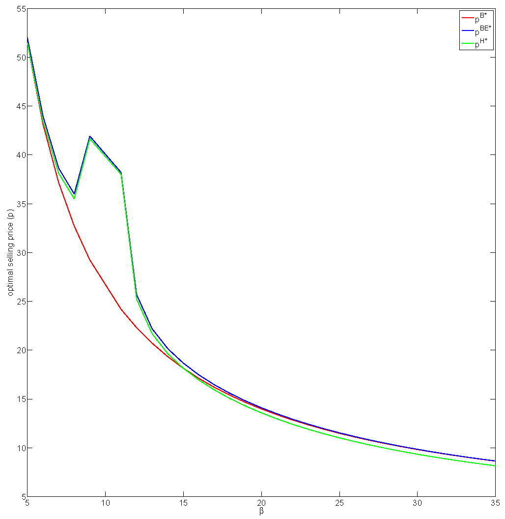
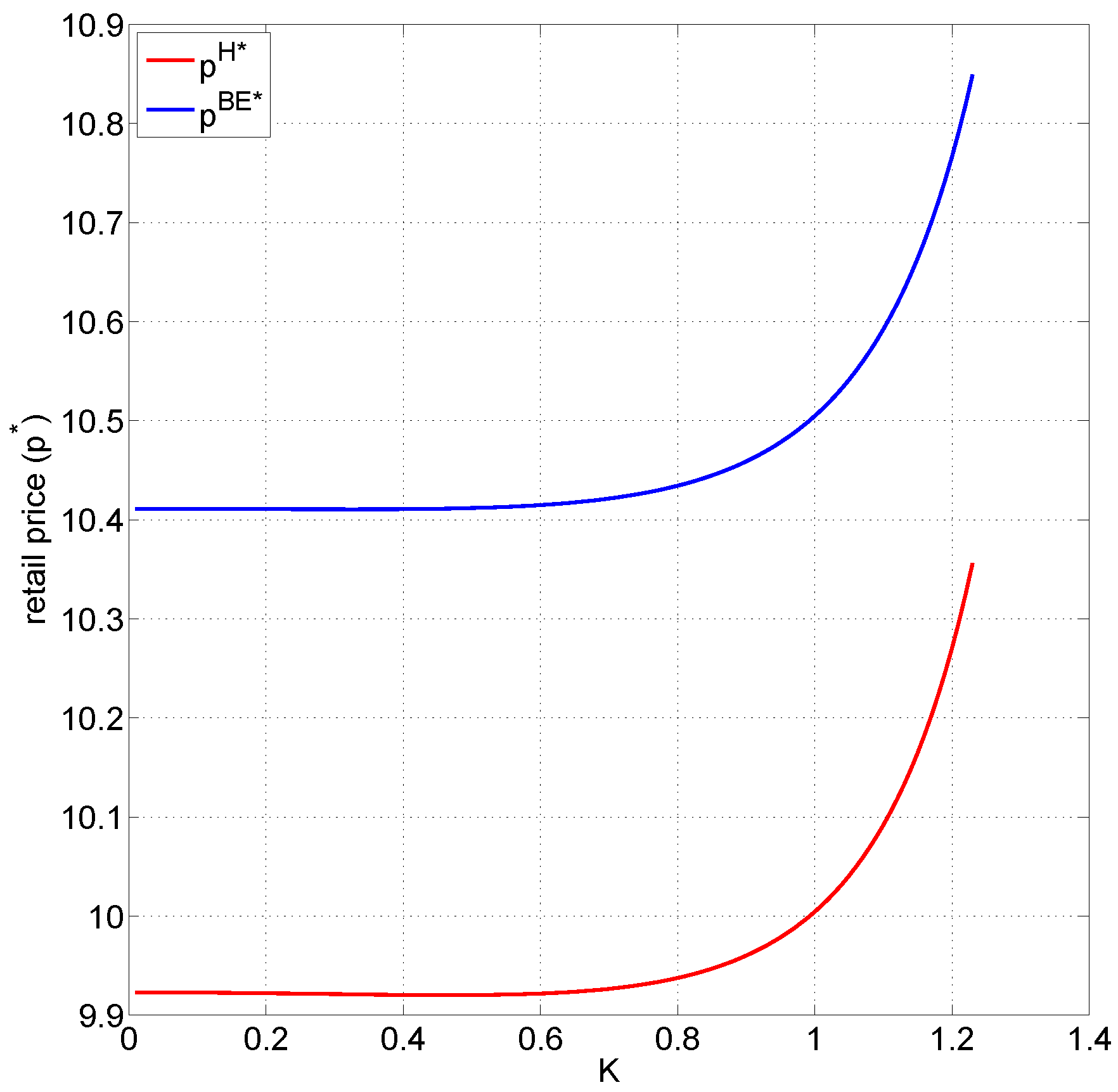
The relationship among the manufacturers’ optimal selling prices is shown in Figure 4.

We can get $p^{BE*}=\frac{\alpha }{\beta }-\frac{2M\left(\alpha -\beta c_m\right)}{4\beta M-4{\beta }^{2}RN}$, $p^{H*}=\frac{\alpha }{\beta }-\frac{2M\left(\alpha -\beta c_m\right)}{4\beta M-4{\beta }^{2}RN-4{\beta }^{2}R{(\Delta -A)}^2}$. Obviously, $p^{B*}>p^{BE*}$. As shown in Figure 4, among the three models, the retail price in model $BE$ is unexpectedly the highest. When the value of $\beta$ is small, $p^{BE*}>p^{H*}>p^{B*}$, which reflects that consumer demand is less sensitive to price, and consumers prefer to purchase the innovation invested products. At this time, both $p^{BE*}$ and $p^{H*}$ have a quicker increase due to the increased cost of innovation input and consumer preference, resulting in an additional increase in retail prices. While the integrated manufacturer considers maximizing consumer utility, it also maximizes his profits. As $\beta$ increases, $p^{BE*}>p^{B*}>p^{H*}$. The retail price of p is relatively small in the hybrid system because the manufacturer can choose to recycle part of the used raw materials from collector 2 with a lower transfer price $b_2$. We assume that the recycled raw materials recovered by the collectors 1, 2 are homogeneous. Therefore, the manufacturer in the hybrid recycling system can save more profit than that in the model $BE$, which is not only the positive impact of recycling innovation investment, but also the social welfare. Another reason is that the manufacturer’s profit in the hybrid model is higher, and some of the profits are derived from the scale effect. In general, the retail price p in the two system models with innovative inputs is not much different from the retail price p in the model without innovative inputs. It shows that innovation investment has not significantly increased retail prices, and can effectively improve channel recovery performance, while increasing consumer demand.

Proposition 3.

The optimal product return rates of different collectors satisfy the following relationship: ${\tau }^{H*}>{\tau }^{BE*}>{\tau }^{B*}$, ${\tau }^{H*}={\tau }_1^{H*}+{\tau }_2^{H*}$, ${\tau }_1^{H*}>{\tau }_2^{H*}$

Interestingly, the total recovery rate of the mixed channel is higher than the basic centralized model, and the manufacturer’s recycling compensation has a direct impact on the collection effort $\tau$. When $b_1^{H*}>b_2^{H*}$, for the two recyclers in the hybrid system, collector 1 has a greater recycling effort. When $b_1^{H*}=b^{BE*}$, the collection rate of collector 1 is greater than the collection rate of the collector in the basic model, the main reason is that the retail price is p. It is precisely because of $p_1^{H*}<p^{BE*}$ that consumer demand is greater. For single-cycle issues, the greater the demand, the greater the scale of recycling generated.

Proposition 4.

The optimal innovation input of collector satisfies the following relationships: $e^{BE*}<e^{H*}$.

Theorem 6.

The manufacturer’s profits under three different modes are related as follows: ${\Pi }_M^{B*}<{\Pi }_M^{BE*}<{\Pi }_M^{H*}$.

Intuitively, manufacturers benefit from increased investment in recycling innovation. Analysis shows that innovation investment not only forces manufacturing to lower retail prices, which leads to higher demand, but also creates more profits for manufacturers by having mixed channels. However, it is counterintuitive that it can be best among integrated manufacturers in the hybrid system.

Such an edge increases when the amount of recyclers in the reverse channel increases, because the scale operated by the integrated manufacturer in model H is higher than that in model $BE$, and the cost savings of recycling and remanufacturing is increased due to collectors competition.

Theorem 7.

The collector’s profits are related as follows, ${\Pi }_{C_1}^{H*}>{\Pi }_C^{BE*}$, ${\Pi }_{C_2}^{H*}>{\Pi }_C^{B*}$.

However, the relationship among ${\Pi }_C^{BE*}$, ${\Pi }_{C_2}^{H*}$ and ${\Pi }_C^{B*}$ is not clear. As mentioned in the assumption of [1], when $c_m-c_r>A$ and $b-A>0$ are satisfied, it is economically viable for recyclers. Reference [13] pointed out that for retailers, even $b_1^{H*}<A$, can compensate for losses by expanding demand. However, for the individual collectors in this article, only through cutting the price A and inflating the transfer price b can they obtain the residual value of the waste products, and expand profits by expanding the demand for recycling. The higher the $\Delta =c_m-c_r$, the higher the return rate $\tau$, the more profitable the recycler will be.

In the market competition environment, in order to gain more market share, some recyclers will improve their recycling efficiency by introducing technological innovations, increasing recycling efforts, and expanding recycling scale and other business strategies to gain competitive advantage.

Theorem 8.

The profits of the supply chains are related as follows: ${\Pi }_T^{B*}<{\Pi }_T^{BE*}<{\Pi }_T^{H*}$.

Interestingly, the supply chain profit is the highest in the hybrid system with two collectors in comparison to the basic centralized channel vertical Stackelberg equilibrium. Thus, competition of collectors through the investment of innovation input is advantageous for the supply chain.

5.2. Numerical Analysis

In this section, we present numerical simulations to illustrate the analytical results of those two models with the innovation input as shown above. We will illustrate the effects of the marginal demand coefficient K and the cost coefficient R on the analytical results in both closed-loop supply chains with innovation input successively.

5.2.1. Impact of Marginal Demand Coefficient for Recycling Innovation Inputs

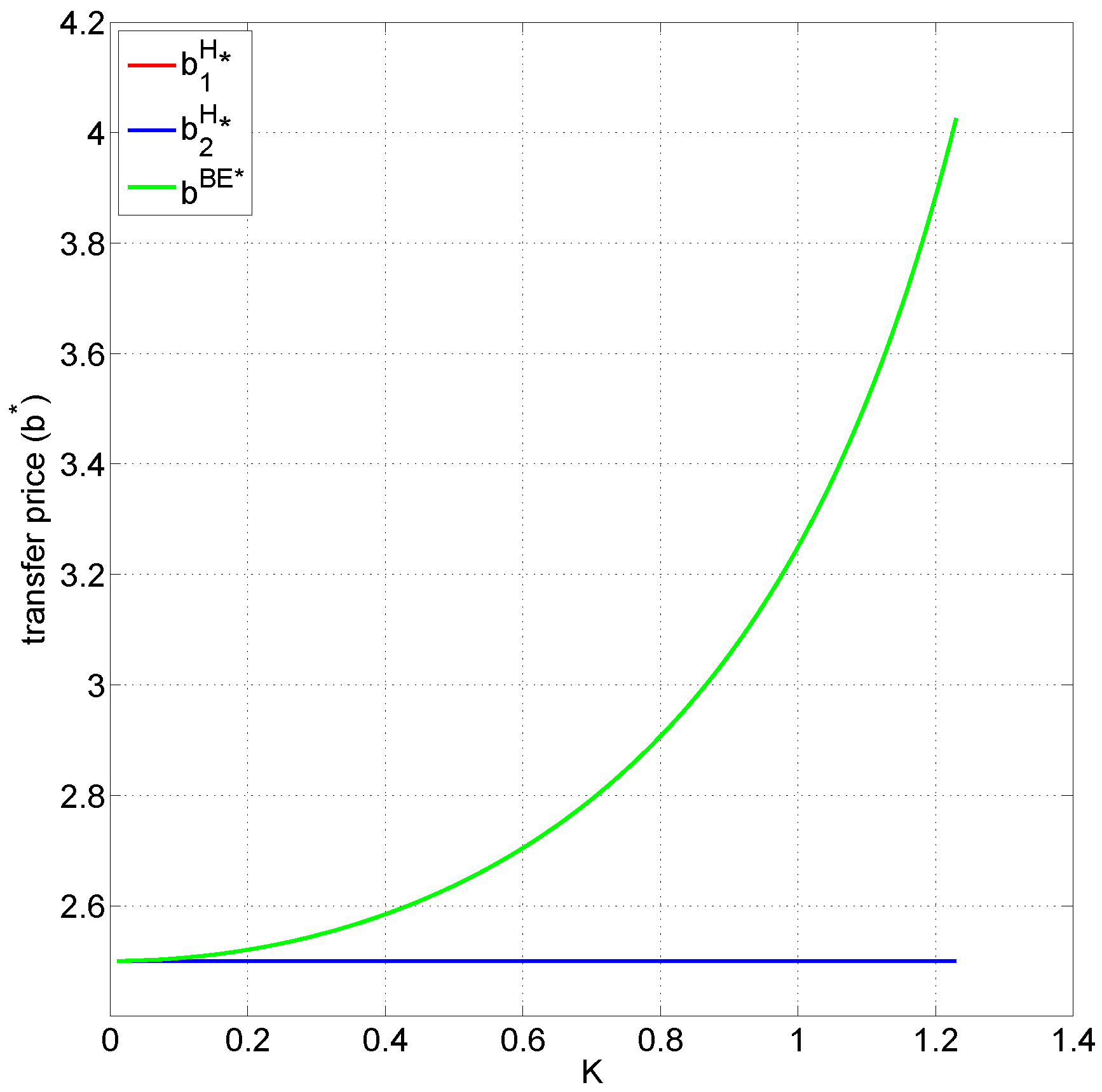
First, we mainly focus on the investigation of K, the marginal demand coefficient for recycling innovation inputs, on the performances of the supply chain. The related parameters are assumed that $\alpha =500$, $\beta =30$, $H=1000$, $R=0.1$. The value of K is varied from 0.01 to 1.2.

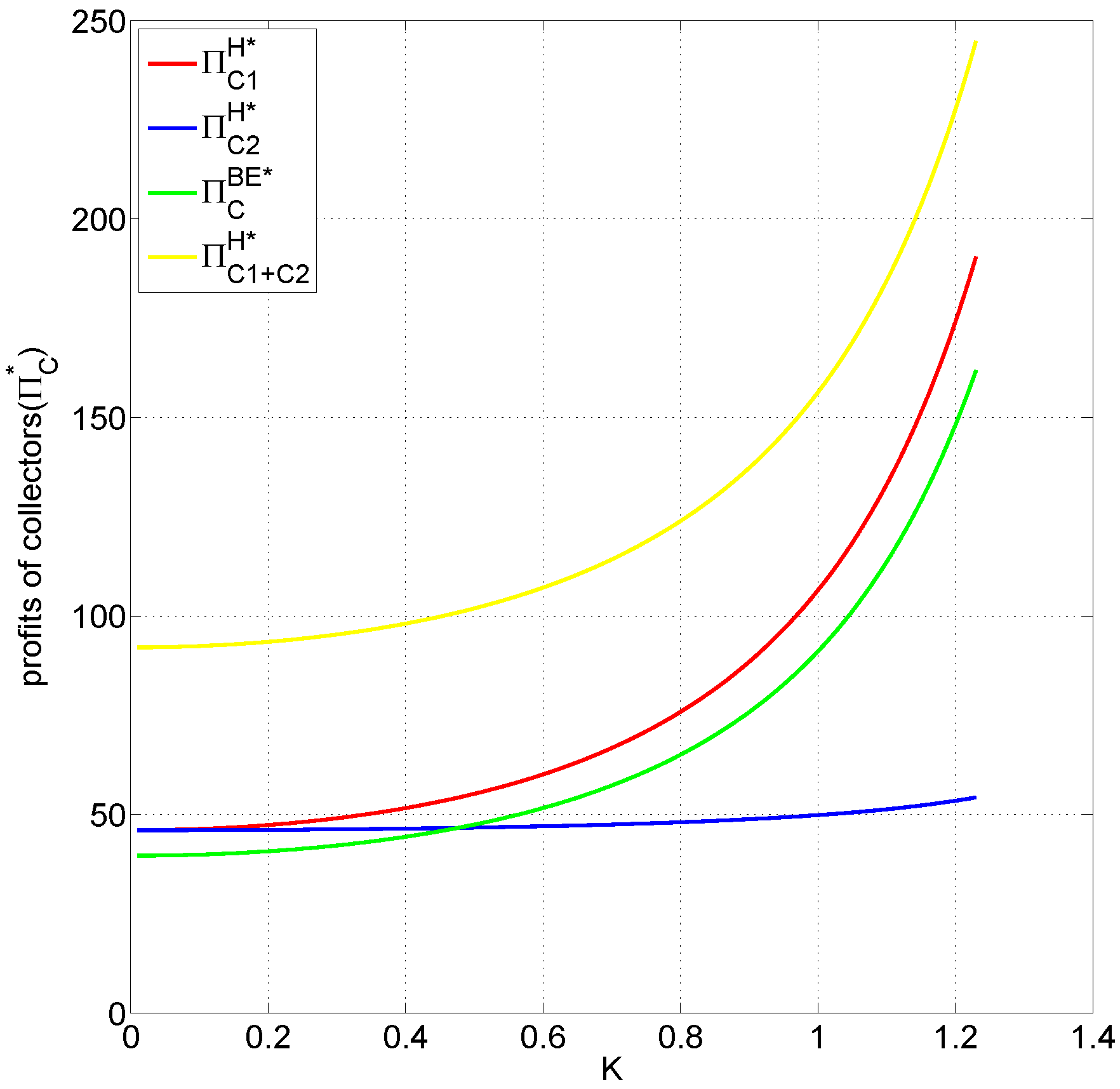
It’s noticed that K has an increasing effect on price, collection effort, innovation input, the profitability of each player, and the total supply chain profits. In Figure 5, as K increases, the transfer prices, $b_1^{H*}$ and $b^{BE*}$ have a climbing trend, while $b_2^{H*}$ stays unchanged, the gap between these two and $b_2^{H*}$ is growing. It means that recyclers expect higher recycling subsidies when they invest in recycling innovations, namely the transfer price of b compensated by the manufacturer.

From Figure 6, considering second scenario, as manufacturer’s share of revenue increases, the products quality of the manufacturer increases and the products quality of the packaging company goes down. When $K<0.6$, the growth of p is flat. When K is greater than 0.6, the growth rate of product selling price goes up but the relationship of $p^{H*}<p^{BE*}$ still remains.

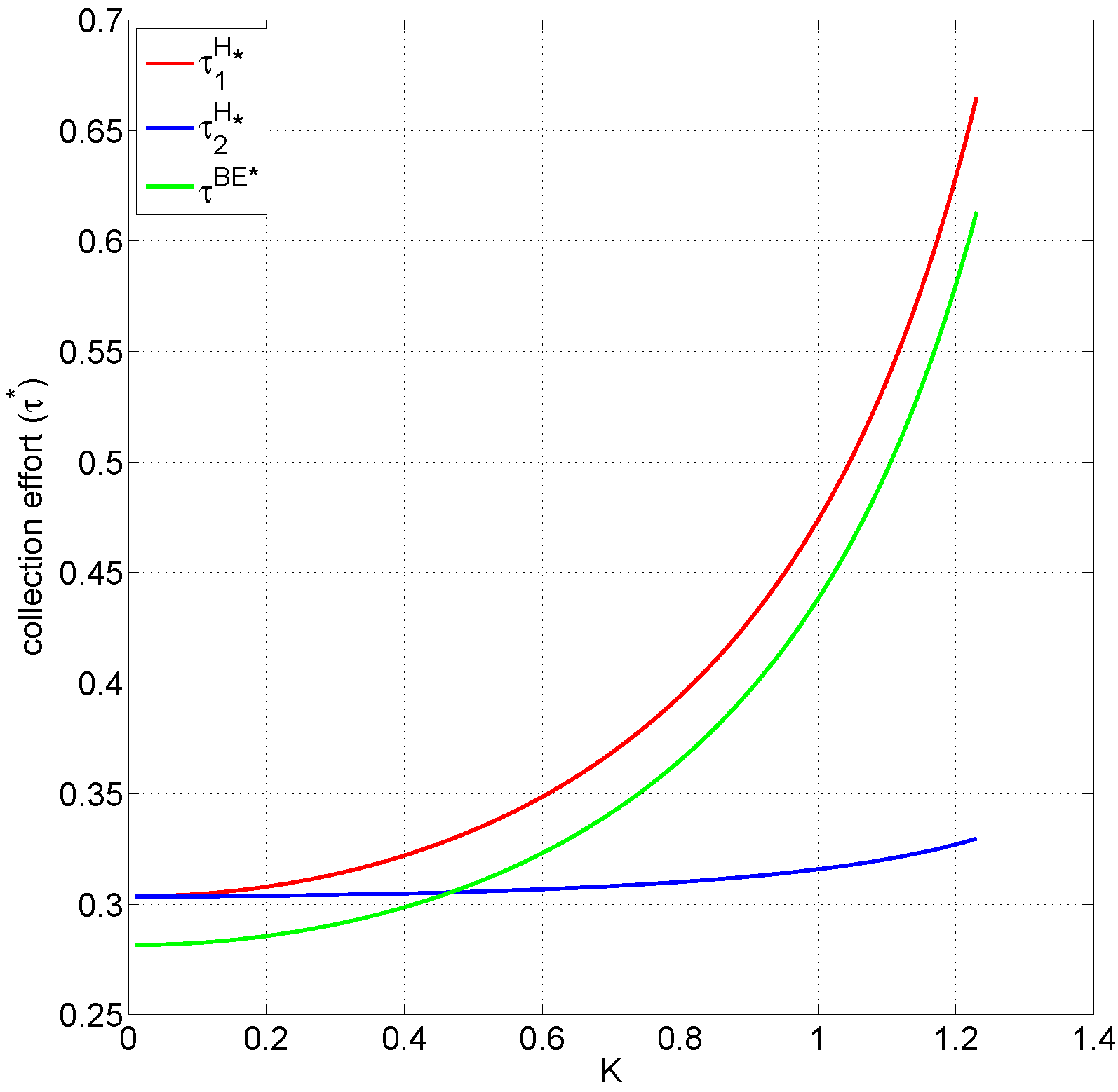
As shown in Figure 7, by increasing K, the innovation input $e^{H*}$ and $e^{BE*}$ also increase, and the rate of growth is getting higher. At the same K level, the innovation input incentive of model H is slightly greater than that of model $BE$. In other words, $e^{H*}$ is slightly higher than $e^{BE*}$ at a comparable K level. However, when model $BE$ is at a high level of K, the innovation input can exceed that of the model H.

Figure 8 shows even though collector 2 does not invest in innovation, its collection rate increases slowly with the increase of K, mainly because of the positive externality brought by innovation input, that is, the social welfare brought by innovation input. When K is low, it means that the collector is in the initial stage of investment collection innovation, ${\tau }_1^{H*}$ is close to ${\tau }_2^{H*}$, it is difficult to see the changes that innovation investment will bring to the collection rate in the short term. Surprisingly, both ${\tau }_1^{H*}$ and ${\tau }_2^{H*}$ are higher than ${\tau }^{BE*}$, we find that when K is at a low level, collector 2 charges the manufacturer a lower transfer price, which saves more cost for the manufacturer to recycle. The manufacturer’s preference also encourages collector 2 to maintain a higher collection rate level. And $e^{H*}$ is slightly higher than $e^{BE*}$, it makes ${\tau }_1^{H*}$ higher than ${\tau }^{BE*}$. However, when K gradually increases, it means that the collectors have entered the development stage of investment and recovery of innovative investment, and the positive impact of recycling innovative investment is becoming more and more obvious. ${\tau }_1^{H*}$ and ${\tau }^{BE*}$ grow rapidly with the increase of K, and ${\tau }^{BE*}$ will soon exceed ${\tau }_2^{H*}$. Therefore, the increasing trends for ${\tau }_1^{H*}$ and ${\tau }^{BE*}$ are similar. We compare collector 2’s performance under the cases with (without) innovation input and can find that the marginal demand coefficient K has significant influence on $\tau$ with innovation input.

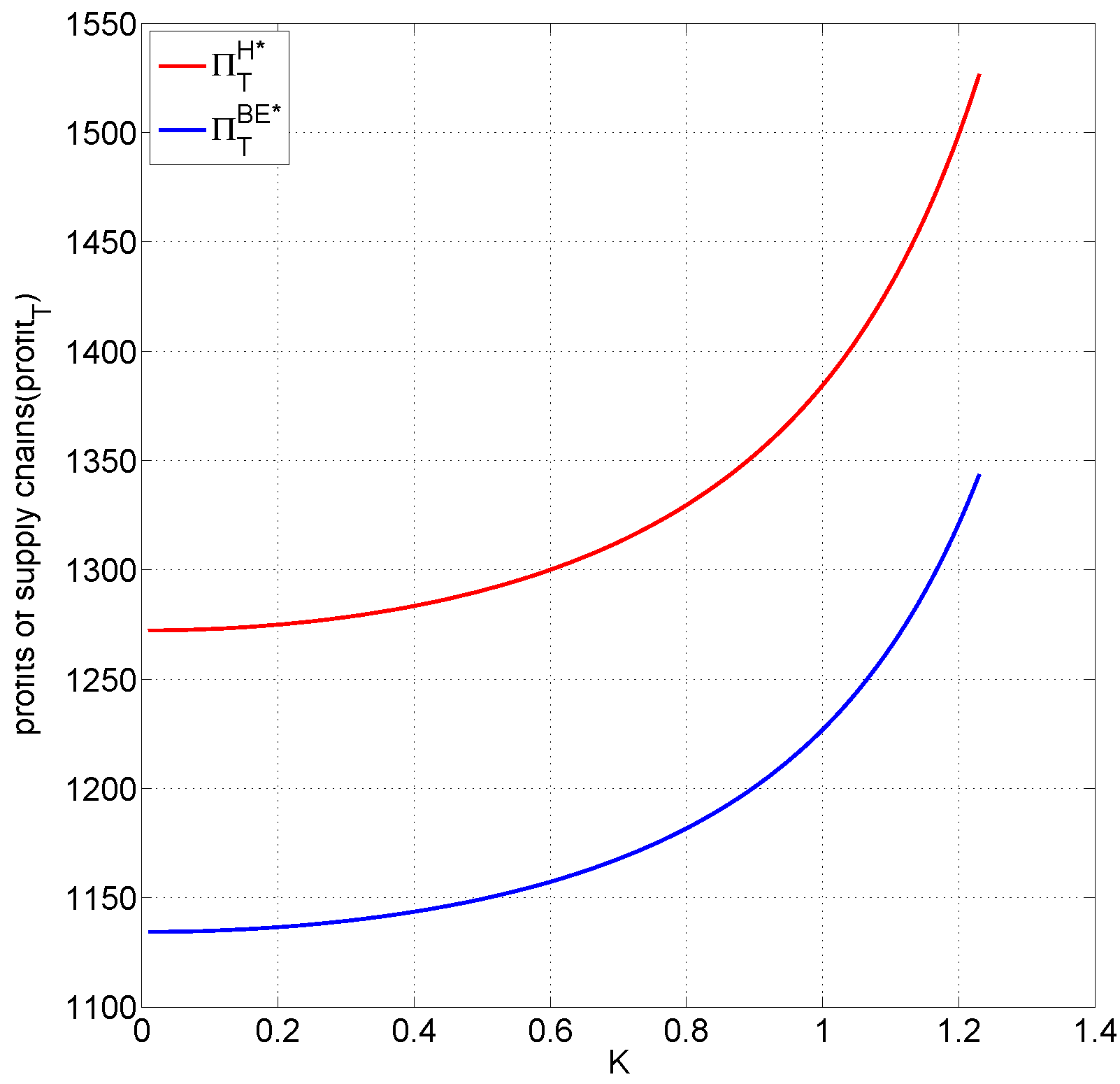
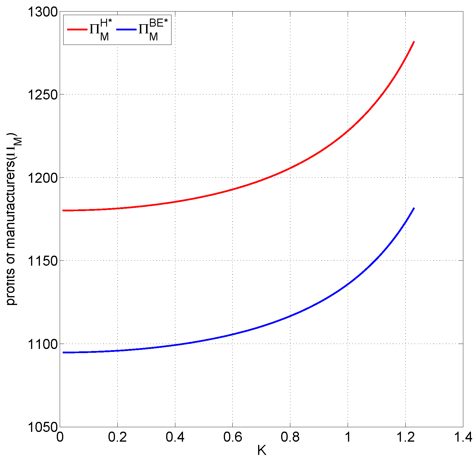
Comparison of total supply chain profits shows the following relationship: ${\Pi }_T^{H*}>{\Pi }_T^{BE*}$. Interestingly, the supply chain profit is higher in the hybrid system with two collectors in comparison to the basic centralized channel vertical Stackelberg equilibrium in Figure 9. Thus, competition of collectors through the investment of innovation input is advantageous for the supply chain. We further compare the individual players’ profits in the two models. In Figure 10, the manufacturer’s profits are in the following order, ${\Pi }_M^{H*}>{\Pi }_M^{BE*}$.

The reason for larger profit of the manufacturer in model H is the increased social welfare brought about by the increased investment in recycling innovation. Due to the externality of innovation investment, the recycling volume of collector 2 without innovation investment will also be improved to a certain extent. For example, the social awareness of environmental recycling is enhanced, and manufacturers can purchase second-hand products or waste materials from collector 2 at a lower price. Then the manufacturers’ profits could be further improved, and also the manufacturers are more willing to sell new products to consumers at lower retail prices.

The collectors’ profits cannot be established. In Figure 11, collector 1 incurs the highest profit in the hybrid system with innovation input. With the increase of K, it means that the positive external influence brought by innovation investment increases, and the profit of the collector increases with the increase of K. Even if collector 2 does not invest in innovation investment, his profit is slowly increasing with the increase of K, which is mainly due to the positive external response brought by the innovation input. It can also be said that the innovation input brings social welfare.

When the K is low, it means that the collector is in the initial stage of investment and innovation investment, and the profits’ relationship between each collector is as follows: ${\Pi }_{C1}^{H*}>{\Pi }_{C2}^{H*}>{\Pi }_C^{BE*}$. Correspondingly, the collection rate relationship among various collectors can be observed: ${\tau }_1^{H*}>{\tau }_2^{H*}>{\tau }^{BE*}$, which means that it is difficult for recycling companies to invest in innovation in the recycling market at first. The conclusions are drawn that the third-party recycling channel is the most unfavorable. Because it often bears a huge amount of innovation input costs when it does not achieve sufficient recycling to make a profit. However, the amount of waste items in society is getting higher and higher. Recycling must also be specialized. The establishment of recycling enterprises is an inevitable trend. Of course, it will require the joint assistance of the government, manufacturing enterprises, and remanufacturing enterprises.

When the K increases, it means that the collector has entered the development stage of investment and recycling innovative inputs, the market environment for innovative inputs is relatively good, and people also prefer recycling channels that contain innovative inputs. We observe that the sorting of the profit size of collectors has changed, ${\Pi }_{C1}^{H*}>{\Pi }_C^{BE*}>{\Pi }_{C2}^{H*}$. The corresponding recovery rate also changes as follows. ${\tau }_1^{H*}>{\tau }^{BE*}>{\tau }_2^{H*}$.

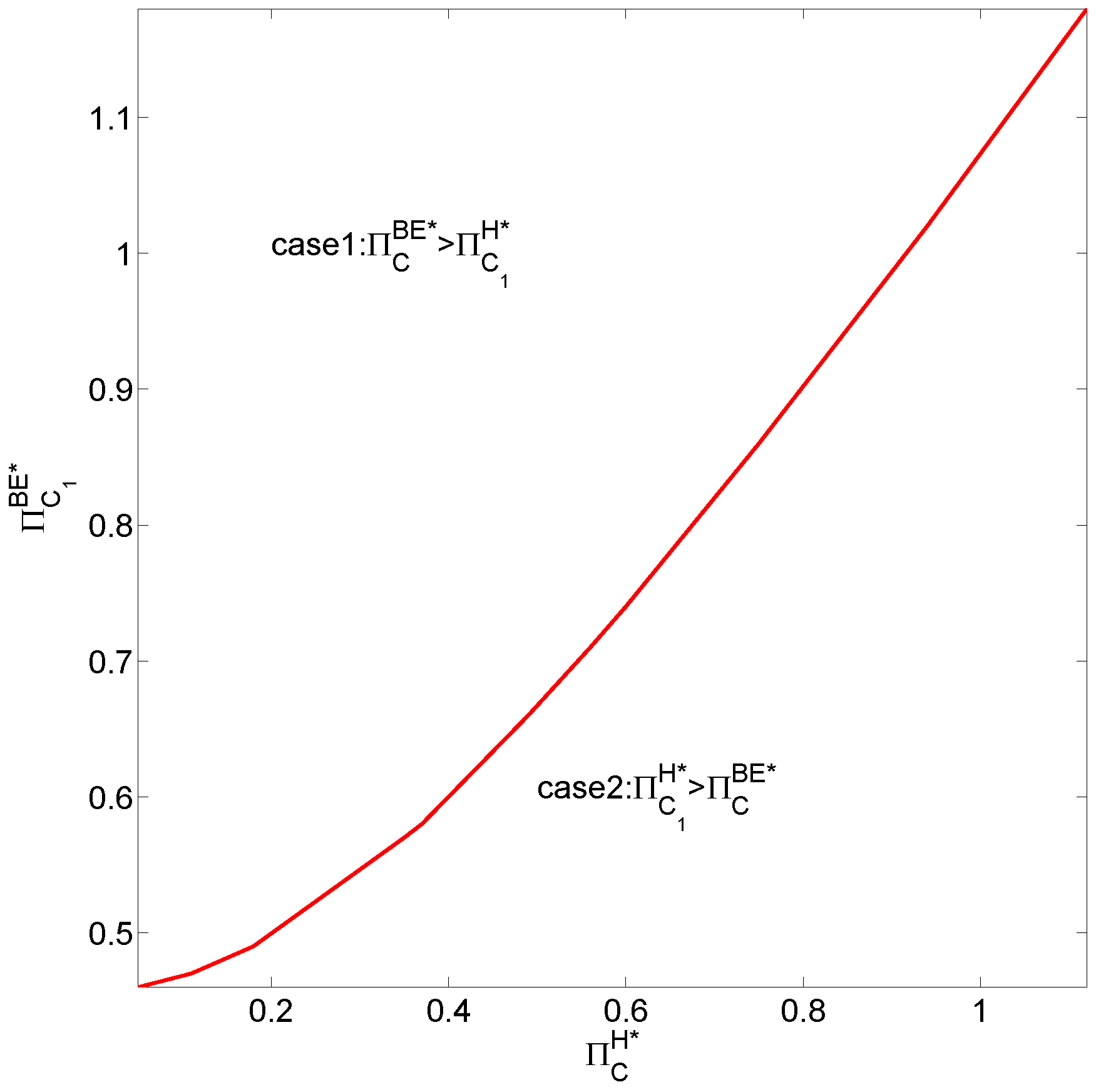
In Figure 12, we study the two collectors’ profits with innovation input and determine regions where its profit is highest relative to K. In the same value of K, ${\Pi }_C^{H*}>{\Pi }_C^{BE*}$. When model $BE$ and model H are in the different K levels, we assume $K_g(g=BE,H)$, subscript g represents the value of K under model $BE$ and model H respectively, which also shows the different market environment responses to innovation input. As the relative $K_H$ increases, we find that case 2 is more profitable for the collector 1 in model H. We find, at higher relative level of $K_{BE}$, case 1 is more profitable than case 2 for the collector in the model $BE$. In case 1, since $K_{BE}$ is more powerful, the collector also dispenses relatively higher effort and also charges higher transfer price leading to higher profits.

Proposition 5.

The profit of each member increases with the increase of K. Interestingly, the hybrid recycling system is superior to the basic centralized recycling model, ${\Pi }_T^{H*}>{\Pi }_T^{BE*}$. In this sense, horizontal competition (at collector level) enhances the sustainability goals. The $e^{*}$ and ${\tau }^{*}$ of competing collectors’ case are also greater than the optimal $e^{*}$ and ${\tau }^{*}$ in the monopoly case. From the perspective of the collector, ${\Pi }_C^{BE*}$ is not only less than ${\Pi }_{C1}^{H*}+{\Pi }_{C2}^{H*}$, but also less than ${\Pi }_{C1}^{H*}$, and in some cases less than ${\Pi }_{C2}^{H*}$. From the manufacturer’s perspective, ${\Pi }_M^{H*}>{\Pi }_M^{BE*}$.

5.2.2. Impact of Cost Factor for Recycling Innovation Inputs

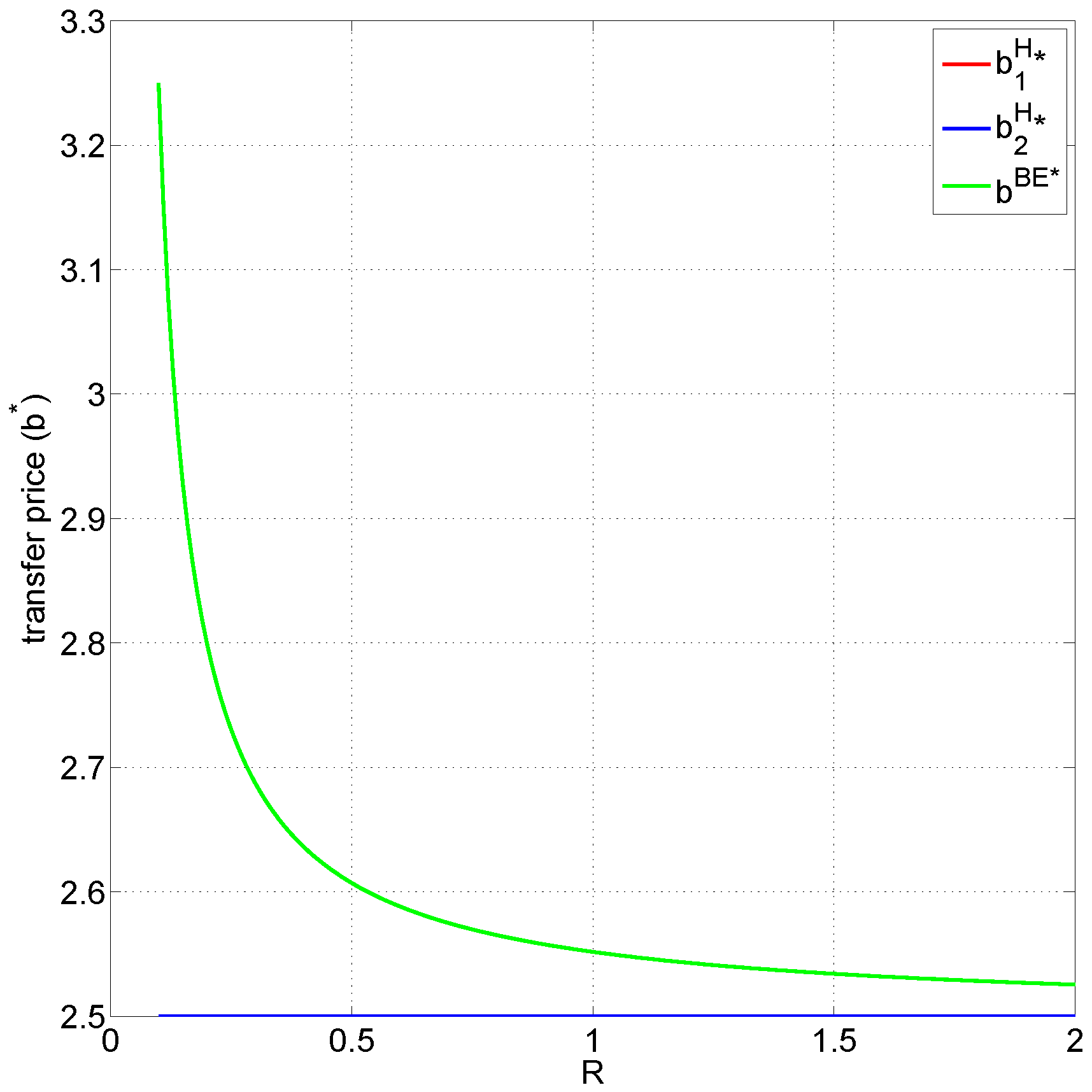
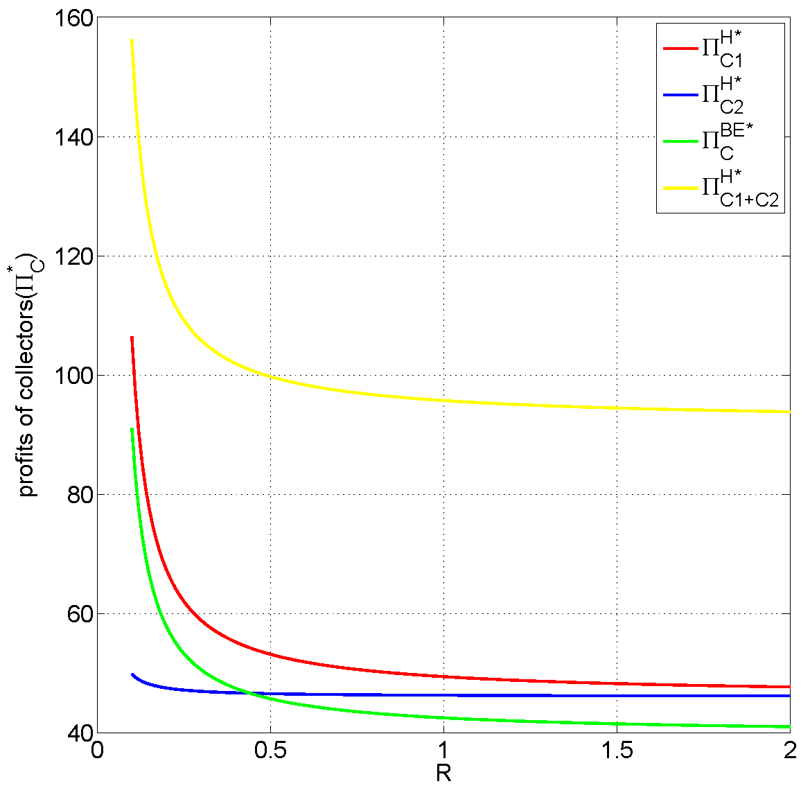
Next, we mainly focus on the investigation of R, the cost factor for recycling innovation inputs, on the performances of the supply chain. The related parameters are assumed that $\alpha =500$, $\beta =30$, $H=1000$, $K=1$. The value of R is varied from 0.01 to 2.

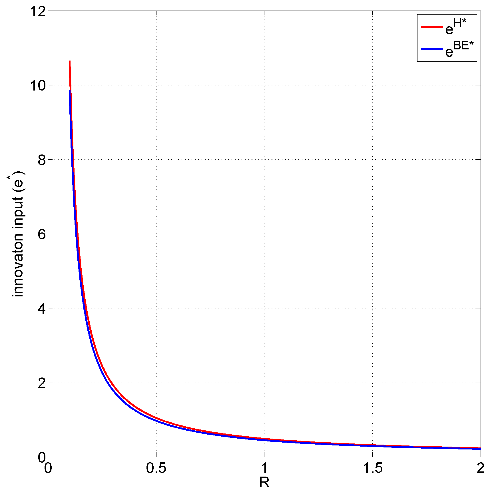
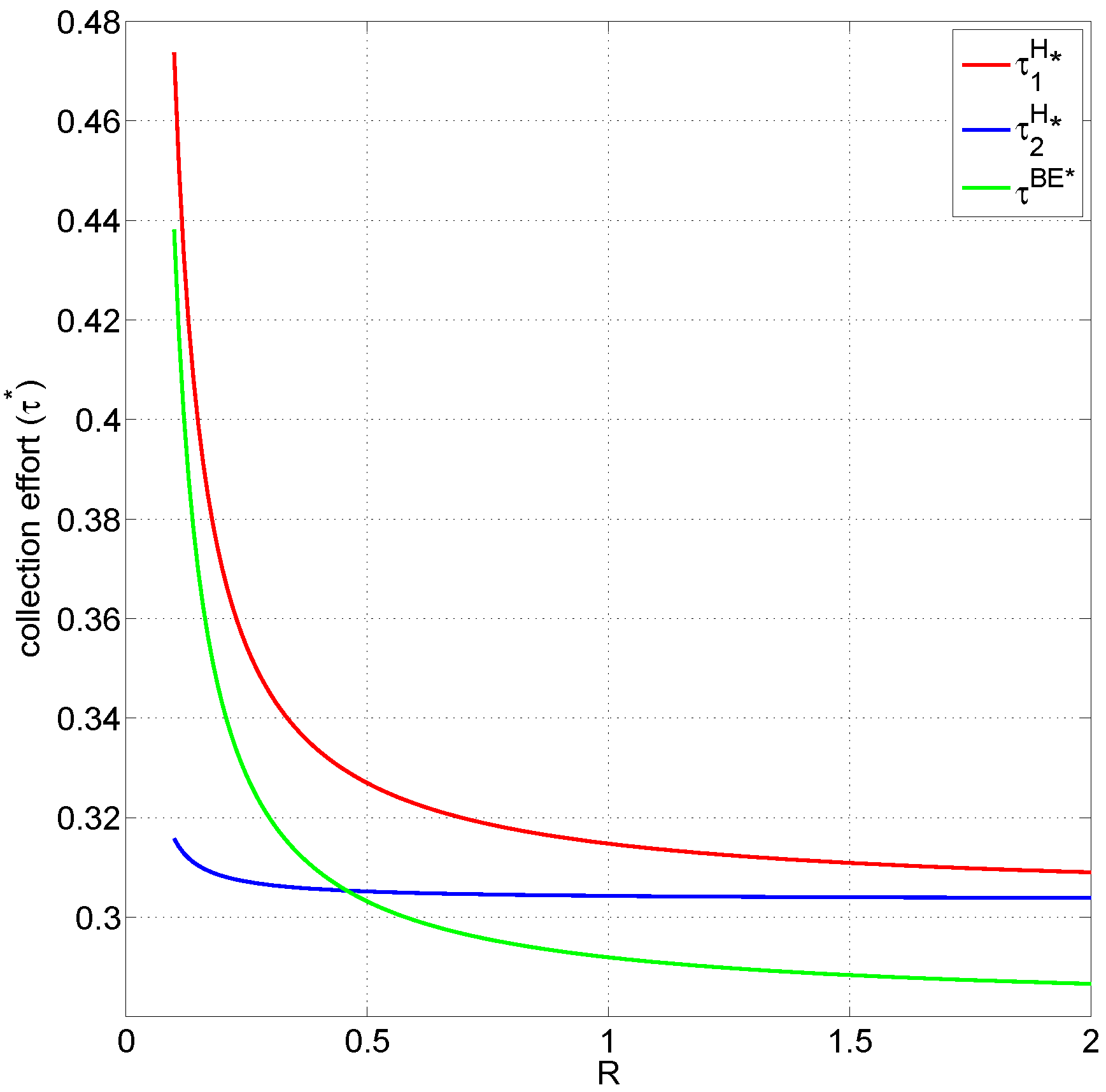
It is noticed that the optimal level of environmental sustainability of the reverse channel and the direct sale channel, the optimal retail price and the optimal direct sale price decrease with the increase of the cost factor R. In Figure 13, $b_1^{H*}$ and $b^{BE*}$ decrease with the increase of R, and the gap with $b_2^{H*}$ gradually decreases. $b_2^{H*}$ remains the same as R increases.

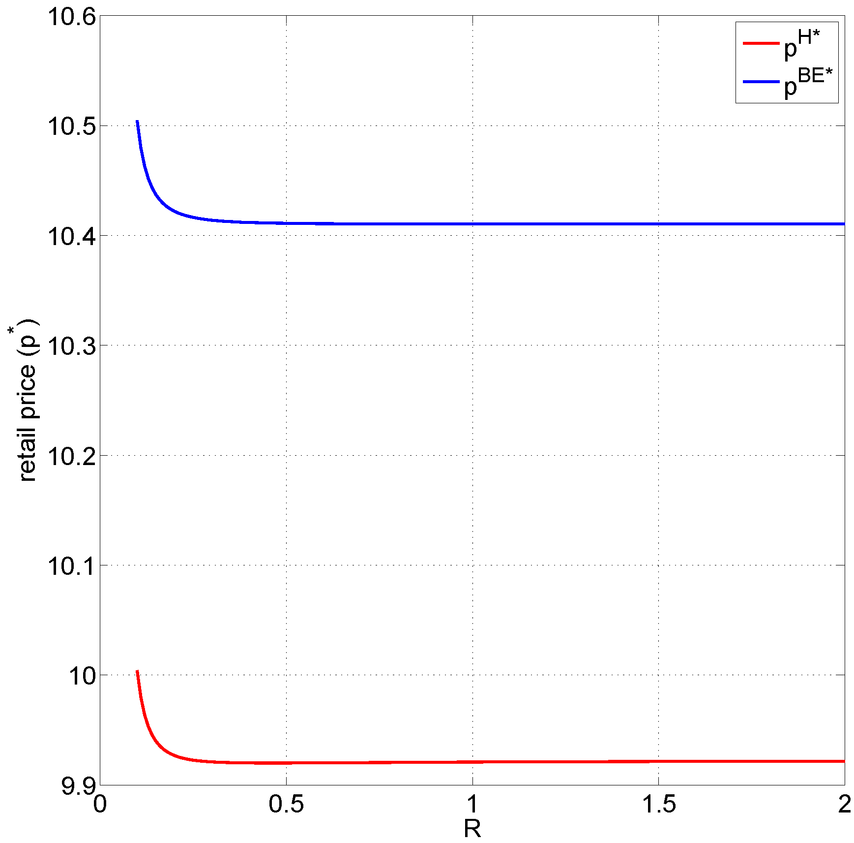
As shown in Figure 14, $p^{H*}$ and $p^{BE*}$ decrease with the increase of R. When $R<0.2$, the decrease rate of p is higher. When R exceeds 0.2, the decrease of p is relatively slow, but it remains $p^{H*}<p^{BE*}$.

In Figure 15, $e^{H*}$ and $e^{BE*}$ decrease with the increase of R, and the rate of decrease becomes smaller and smaller. When at the same R value level, the incentive for innovation input of model H is slightly higher than that in model $BE$, that is, $e^{H*}>e^{BE*}$. However, when the value of R in model $BE$ is at a lower level, the investment in innovation can exceed that in model H.

It can be seen from Figure 16 that even if collector 2 does not invest in innovation, his collection rate also slowly decreases with the increase of R, which means that the cost coefficient of innovation input has a certain impact on collector 2, but the impact is not great. When the R is low, it means that the collector’s investment to recover the innovation input is low, which is an ideal situation with low investment and high return. ${\tau }_1^{H*}$ and ${\tau }^{BE*}$ are at the highest level, both are higher than ${\tau }_2^{H*}$. It can also be seen that if you want to promote recycle companies to carry out recycling innovation investment, reducing innovation investment costs is a fast-acting method. However, when the R gradually increases, it means that the cost of investing in recycling innovation investment by collectors is gradually increasing, and the barriers to entering the innovation recycling market are gradually rising. Recycling efforts ${\tau }_1^{H*}$ and ${\tau }^{BE*}$ declined rapidly, and ${\tau }^{BE*}$ even gradually fell below ${\tau }_2^{H*}$. At the same time, we also observe that the cost coefficient of innovation investment e is increasing, and the decreasing trends of ${\tau }_1^{H*}$ and ${\tau }^{BE*}$ are more consistent. Compared with the collector 2 without innovation investment, the rate of decrease is greater. It shows that R has a significant impact on $\tau$ with innovation inputs. It also reflects that the excessively high cost of innovation input hinders the recycler’s innovation investment in the recycling market.

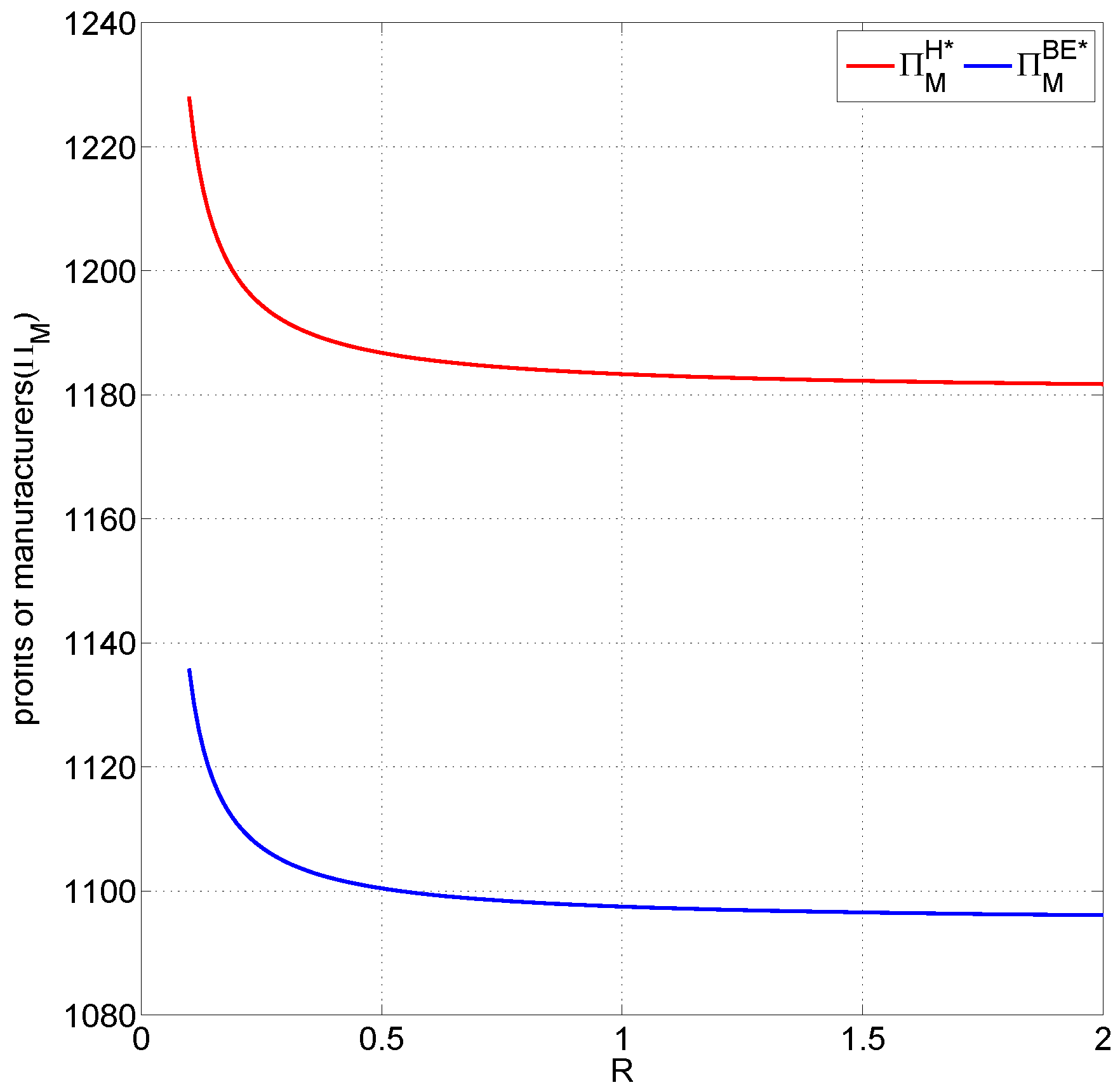
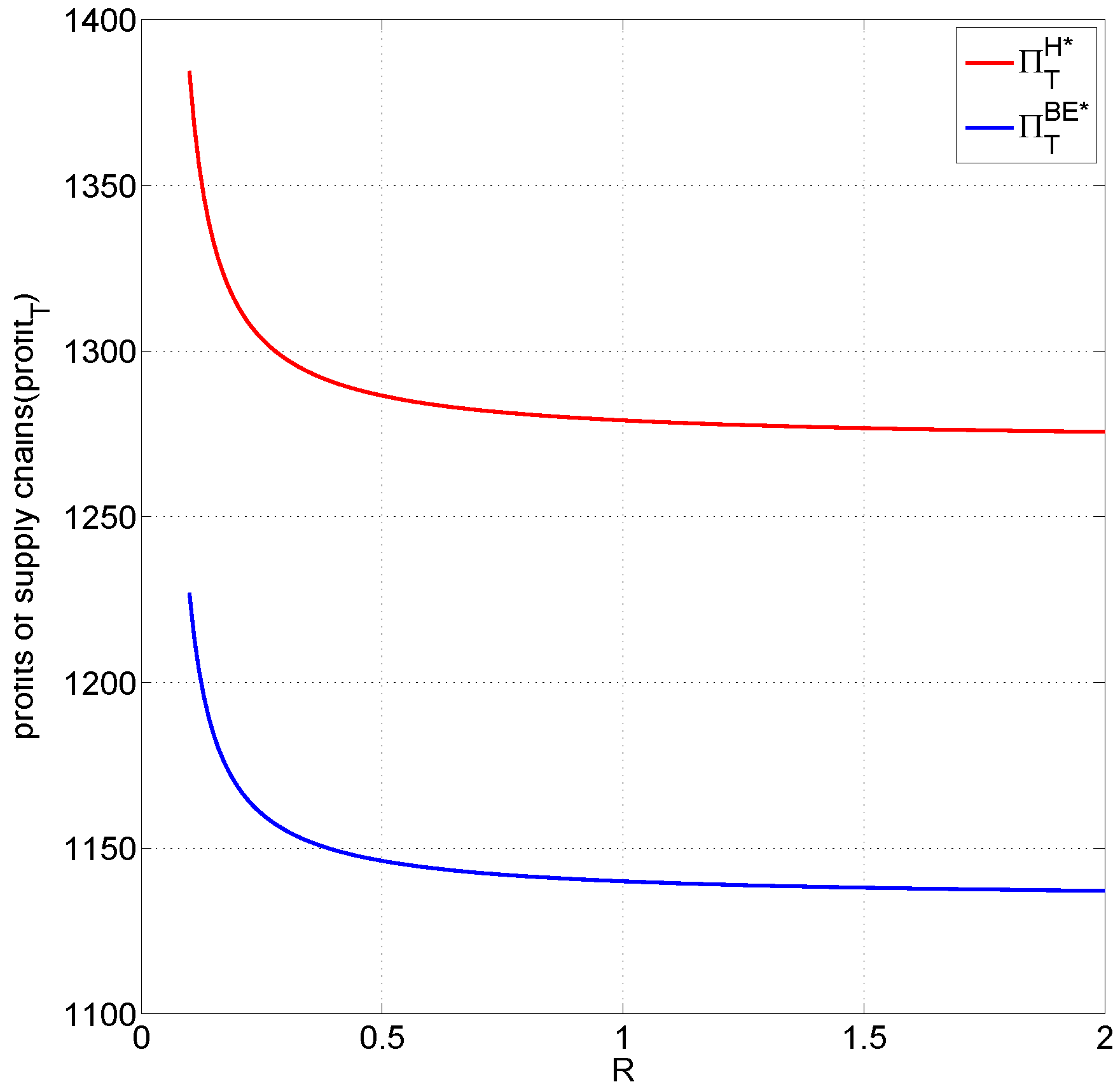
From Figure 17 and Figure 18, comparison of total supply chain profits and manufacturer’s profits show the following relationship: ${\Pi }_T^{H*}>{\Pi }_T^{BE*}$, ${\Pi }_M^{H*}>{\Pi }_M^{BE*}$.

The increase in the investment in recycling innovation has led to an increase in social welfare, which has led to greater profits for the manufacturer in Model H. The recovery volume and recovery rate of collector 2 without innovation input are improved to a certain extent because of the positive externality of innovation input. For example, the emergence of intelligent recycling bins and the Internet Plus recycling platform have increased the environmental recycling awareness of the society, and the overall recycling volume of the society has risen. The manufacturer can purchase second-hand or used materials from collector 2 at a lower transfer price. Therefore, the cost savings of the manufacturer’s recycling and remanufacturing are further reduced, and consequently, profits are further improved. The manufacturer is more willing to sell new products to consumers at lower retail prices.

The collectors’ profits can not be established. From Figure 19, collector 1 incurs the highest profit in the hybrid system with innovation input. With the increase of R, it indicates that the cost of innovation input gradually increases, while the profit of the recycler decreases. Even if collector 2 does not invest in recycling innovation, his profit slowly decreased with the increase of R. When the value of R is low, it reflects that the recycler invests less cost for recycling innovation. The profit relationship between each recycler is as follows: ${\Pi }_{C1}^{H*}>{\Pi }_C^{BE*}>{\Pi }_{C2}^{H*}$. Correspondingly, we can observe the recovery rate relationship among various recyclers: ${\tau }_1^{H*}>{\tau }^{BE*}>{\tau }_2^{H*}$. It is shown that recyclers have just started to innovate in the recycling market with low input costs, low barriers to entry, and large gains. With the influx of a large number of collectors into the market, the competition for recycling innovation is fierce. Correspondingly, the cost of innovation investment has increased. When R gradually increases, it indicates that the cost of investing in recycling innovation investment by collectors is relatively high, greatly reducing the enthusiasm of collectors for innovation investment. However, due to the lack of recycling volume, which cannot compensate for the losses caused by the cost of innovation input, we find that the sorting of the profit size of the collectors has changed, ${\Pi }_{C1}^{H*}>{\Pi }_{C2}^{H*}>{\Pi }_C^{BE*}$. The recovery rate also changes as follows, ${\tau }_1^{H*}>{\tau }_2^{H*}>{\tau }^{BE*}$, correspondingly.

Proposition 6.

The profits of each member decreases with the increase of R. Interestingly, the hybrid recycling system is superior to the basic centralized recycling model, ${\Pi }_T^{H*}>{\Pi }_T^{BE*}$. The $e^{*}$ and ${\tau }^{*}$ of competing collectors’ case are also greater than the optimal $e^{*}$ and ${\tau }^{*}$ in the monopoly case. From the perspective of the collector, ${\Pi }_C^{BE*}$ is not only less than ${\Pi }_{C1}^{H*}+{\Pi }_{C2}^{H*}$, but also less than ${\Pi }_{C1}^{H*}$, and in some cases less than ${\Pi }_{C2}^{H*}$. From the manufacturer’s perspective, ${\Pi }_M^{H*}>{\Pi }_M^{BE*}$.

Comparing the two settings, we can find that the optimal level of collection effort, innovation input of collector, the retail price, the transfer price and the total profit of the supply chain in the basic centralized model are always lower than those in the hybrid model. The vertical externality effect not only affects the profits of the supply chain and members but also influences the collection effort of the collector with or without innovation input.

Proposition 7.

When the market conditions of K are large and R is low, it is very beneficial to the development of recycling innovation, and the social welfare brought by recycling innovation investment is also high.

6. Concluding Remarks

Whether the collector recycles innovation input will lead to different channel performance. We explore the importance of innovative investment for recycling and the supply chain. By analytically addressing the three important research questions we proposed in the introduction section, this paper has made two important contributions as listed below.

1.

In the previous literature, it was mentioned that third-party recycling channels are often not the best choice. However, in the era of the Internet Plus third-party recycling platforms have received more attention. When compared to the basic model without innovation input, both the model $BE$ and the model H enhance product collection rate and players’ profits in the game. Due to the externality of innovation investment, it will simultaneously increase the positive demand of products and the profit of the integrated manufacturers. We can easily find out many practical applications in the business world. The model B and the model $BE$ are suitable for competition between brands with different recycling innovation inputs like well-known brands and store brand. Such as Ai Hui Shou, the largest O2O electronic product recycling and trade-in service internet platform in China, compete against their local recovery points. It has close collaborations with e-business platforms (like JD.com) and smartphone producers (like SAMSUNG). Consumers can choose the trade-in program to replace an old smartphone with a new one. Moreover, that kind of competition widely exists in many other countries. Such as the case of horizontal competition between Germany Reisman and the local recovery points.

2.

The integrated manufacturer can share the recycling costs of recyclers by setting b (transfer payment price), when the manufacturer recycles second-hand products or raw materials from two competing collectors in either the same market or different markets, the optimal collection rate and innovation input will increase as a result of the horizontal competition between the two collectors. This kind of cost-sharing contract theme is also very popular in practical applications. For instance, Hisense has adopted different transfer price strategies for Shandong Zhonglv and the other local recyclers. In addition, the competitive companies with different recycling innovation inputs have brought a huge boost to the phone’s recycling market. Different pricing mechanisms are adopted by Huawei and Xiaomi for different recyclers, like Da Ba Shou and the other local recovery points.

This study could be extended on several possible aspects. First, we assume a manufacturer that integrates retailers together to weaken the sales process in order to highlight the recycling process. However, some recycling and manufacturing processes are inseparable in some real practice. Second, throughout this paper, we consider a supply chain system in which a monopolist manufacturer collects through a single collector or two collectors. It is likely to observe horizontal competitions between collectors or manufacturers. Finally, we assume all the information is symmetric between both firms throughout this study, but in some situations, the manufacturer is likely more informed about the investment cost, whereas the retailer can be more knowledgeable about the demand. These complexities will undeniably affect the strategic interaction between the manufacturer and collector. Thereby altering the role played in our current CLSC setting. It would be interesting to include these factors into our model in the future.

For future research, although our model is well-supported by the literature and also well-motivated by various industrial practices, we have made a few assumptions that could be relaxed in future research. For example, in our mode, the recycling performance of a single recycler is fixed, but for recyclers with innovative inputs, his recycling input is reproducible and expandable. When the recycler succeeds in a certain area, the business model can be expanded rapidly. We only consider the problem of a single recycler’s innovation efforts in a single system, and further efforts to apply this investment to n systems. In addition, since we only examine the deterministic CLSC models, it is interesting while challenging to extend the work to the stochastic case and important issues can be explored, such as how the randomness and nonlinearity affect the supply chain agents’ decisions and performance, and how the degrees of risk aversion or alternative risk-related optimization objectives of different supply chain agents affect the supply chain performance.

References

- Savaskan, R.C.; Bhattacharya, S.; Van Wassenhove, L.N. Closed-loop supply chain models with product remanufacturing. Manag. Sci. 2004, 50, 239–252. [Google Scholar] [CrossRef] [Green Version]
- Nicolli, F.; Johnstone, N.; Söderholm, P. Resolving failures in recycling markets: The role of technological innovation. Environ. Econ. Policy Stud. 2012, 14, 261–288. [Google Scholar] [CrossRef]
- Choi, T.M.; Li, Y.; Xu, L. Channel leadership, performance and coordination in closed loop supply chains. Int. J. Prod. Econ. 2013, 146, 371–380. [Google Scholar] [CrossRef]
- Chuang, C.; Wang, C.X.; Zhao, Y. Closed-loop supply chain models for a high-tech product under alternative reverse channel and collection cost structures. Int. J. Prod. Econ. 2014, 156, 108–123. [Google Scholar] [CrossRef]
- Giri, B.C.; Chakraborty, A.; Maiti, T. Pricing and return product collection decisions in a closed-loop supply chain with dual-channel in both forward and reverse logistics. J. Manuf. Syst. 2017, 42, 104–123. [Google Scholar] [CrossRef]
- Wang, J.; Jiang, H.; Yu, M. Pricing decisions in a dual-channel green supply chain with product customization. J. Clean. Prod. 2020, 247, 119101. [Google Scholar] [CrossRef]
- Mondal, C.; Giri, B.C. Pricing and used product collection strategies in a two-period closed-loop supply chain under greening level and effort dependent demand. J. Clean. Prod. 2020, 265, 121–335. [Google Scholar] [CrossRef]
- Jia, D.; Li, S. Optimal decisions and distribution channel choice of closed-loop supply chain when e-retailer offers online marketplace. J. Clean. Prod. 2020, 265, 121767. [Google Scholar] [CrossRef]
- Ullah, M.; Sarkar, B. Recovery-channel selection in a hybrid manufacturing-remanufacturing production model with RFID and product quality. Int. J. Prod. Econ. 2020, 219, 360–374. [Google Scholar] [CrossRef]
- Wang, N.; Song, Y.; He, Q.; Jia, T. Competitive dual-collecting regarding consumer behavior and coordination in closed-loop supply chain. Comput. Ind. Eng. 2020, 144, 106481. [Google Scholar] [CrossRef]
- Kokkinaki, A.; Dekker, R.; Lee, R.; Pappis, C. Integrating a Web-Based System with Business Processes in Closed Loop Supply Chains; Technical report; Erasmus University Rotterdam: Rotterdam, The Netherlands, 2001. [Google Scholar]
- Tamas, P.; Illes, B.; Banyai, T.; Toth, A.B.; Akylbek, U.; Skapinyecz, R. Intensifying Cross-border Logistics Collaboration Opportunities Using a Virtual Logistics Center. J. Eng. Res. Rep. 2020, 13, 1–7. [Google Scholar] [CrossRef]
- Savaskan, R.C.; Wassenhove, L.N.V. Reverse Channel Design: The Case of Competing Retailers. Manag. Sci. 2006, 52, 1–14. [Google Scholar] [CrossRef] [Green Version]
- Abbey, J.D.; Blackburn, J.D.; Guide, V.D.R., Jr. Optimal pricing for new and remanufactured products. J. Oper. Manag. 2015, 36, 130–146. [Google Scholar] [CrossRef]
- Yi, P.; Huang, M.; Guo, L.; Shi, T. Dual recycling channel decision in retailer oriented closed-loop supply chain for construction machinery remanufacturing. J. Clean. Prod. 2016, 137, 1393–1405. [Google Scholar] [CrossRef]
- Gan, S.S.; Pujawan, I.N.; Widodo, B. Pricing decision for new and remanufactured product in a closed-loop supply chain with separate sales-channel. Int. J. Prod. Econ. 2017, 190, 120–132. [Google Scholar] [CrossRef] [Green Version]
- Huang, M.; Song, M.; Lee, L.H.; Ching, W.K. Analysis for strategy of closed-loop supply chain with dual recycling channel. Int. J. Prod. Econ. 2013, 144, 510–520. [Google Scholar] [CrossRef]
- Zhao, J.; Wei, J.; Li, M. Collecting channel choice and optimal decisions on pricing and collecting in a remanufacturing supply chain. J. Clean. Prod. 2017, 167, 530–544. [Google Scholar] [CrossRef]
- Wei, J.; Wang, Y.; Zhao, J.; Gonzalez, E.D.R.S. Analyzing the performance of a two-period remanufacturing supply chain with dual collecting channels. Comput. Ind. Eng. 2019, 135, 1188–1202. [Google Scholar] [CrossRef]
- Zheng, Y.; Shu, T.; Wang, S.; Chen, S.; Lai, K.K.; Gan, L. Analysis of product return rate and price competition in two supply chains. Oper. Res. 2018, 18, 469–496. [Google Scholar] [CrossRef]
- He, Q.; Wang, N.; Yang, Z.; He, Z.; Jiang, B. Competitive collection under channel inconvenience in closed-loop supply chain. Eur. J. Oper. Res. 2019, 275, 155–166. [Google Scholar] [CrossRef]
- Taleizadeh, A.A.; Sadeghi, R. Pricing strategies in the competitive reverse supply chains with traditional and e-channels: A game theoretic approach. Int. J. Prod. Econ. 2019, 215, 48–60. [Google Scholar] [CrossRef]
- Wang, N.; He, Q.; Jiang, B. Hybrid closed-loop supply chains with competition in recycling and product markets. Int. J. Prod. Econ. 2018, 217, 246–258. [Google Scholar] [CrossRef]
- Liu, Y. Pattern Changes in the Reverse Logistics of Household Appliances in the Light of “Internet Plus” Strategy. China Bus. Mark. 2015, 29, 30–35. [Google Scholar]
- Liu, L.; Wang, Z.; Xu, L.; Hong, X.; Govindan, K. Collection effort and reverse channel choices in a closed-loop supply chain. J. Clean. Prod. 2017, 144, 492–500. [Google Scholar] [CrossRef]
- Wong, D.T.W.; Ngai, E.W.T. Critical review of supply chain innovation research (1999–2016). Ind. Mark. Manag. 2019, 82, 158–187. [Google Scholar] [CrossRef]
- Mallampati, S.R.; Lee, B.H.; Mitoma, Y.; Simion, C. Sustainable recovery of precious metals from end-of-life vehicles shredder residue by a novel hybrid ball-milling and nanoparticles enabled froth flotation process. J. Clean. Prod. 2018, 171, 66–75. [Google Scholar] [CrossRef]
- Li, J.; Barwood, M.; Rahimifard, S. Robotic disassembly for increased recovery of strategically important materials from electrical vehicles. Robot. Comput.-Integr. Manuf. 2018, 50, 203–212. [Google Scholar] [CrossRef] [Green Version]
- Zhao, J.; Wang, C.; Xu, L. Decision for pricing, service, and recycling of closed-loop supply chains considering different remanufacturing roles and technology authorizations. Comput. Ind. Eng. 2019, 132, 59–73. [Google Scholar] [CrossRef]
- Zhang, D.; Zhang, X.; Shi, B.; Cao, J.; Zhou, G. Collection and Remanufacturing of Waste Products under Patent Protection and Government Regulation. Sustainability 2018, 10, 1402. [Google Scholar] [CrossRef] [Green Version]
- Ford, P.; Santos, E.; Ferrão, P.; Margarido, F.; Van Vliet, K.J.; Olivetti, E. Economics of end-of-life materials recovery: a study of small appliances and computer devices in Portugal. Environ. Sci. Technol. 2016, 50, 4854–4862. [Google Scholar] [CrossRef] [Green Version]
- Cao, J.; Xu, J.; Wang, H.; Zhang, X.; Chen, X.; Zhao, Y.; Yang, X.; Zhou, G.; Schnoor, J.L. Innovating Collection Modes for Waste Electrical and Electronic Equipment in China. Sustainability 2018, 10, 1446. [Google Scholar] [CrossRef] [Green Version]
- Bian, J.; Zhang, G.; Zhou, G. Manufacturer vs. Consumer Subsidy with Green Technology Investment and Environmental Concern. Eur. J. Oper. Res. 2020, 287, 832–843. [Google Scholar] [CrossRef]
- Liu, Z.; Anderson, T.; Cruz, J.M. Consumer environmental awareness and competition in two-stage supply chains. Eur. J. Oper. Res. 2012, 218, 602–613. [Google Scholar] [CrossRef]
- Durana, P.; Zauskova, A.; Vagner, L.; Zadnanova, S. Earnings Drivers of Slovak Manufacturers: Efficiency Assessment of Innovation Management. Appl. Sci. 2020, 10, 4251. [Google Scholar] [CrossRef]
- Durana, P.; Valaskova, K.; Vagner, L.; Zadnanova, S.; Podhorska, I.; Siekelova, A. Disclosure of strategic managers’ factotum: Behavioral incentives of innovative business. Int. J. Financ. Stud. 2020, 8, 17. [Google Scholar] [CrossRef] [Green Version]
- Zhang, S.; Wang, C.; Yu, C.; Ren, Y. Governmental cap regulation and manufacturer’s low carbon strategy in a supply chain with different power structures. Comput. Ind. Eng. 2019, 134, 27–36. [Google Scholar] [CrossRef]
- Li, G.; Li, L.; Sun, J. Pricing and service effort strategy in a dual-channel supply chain with showrooming effect. Transp. Res. Part Logist. Transp. Rev. 2019, 126, 32–48. [Google Scholar] [CrossRef]
Figure 1.
The closed-loop supply chain (CLSC) structure of model B.
Figure 2.
The CLSC structure of model .
Figure 3.
The CLSC structure of model H.
Figure 4.
The influences of on the retail price p.
Figure 5.
The influences of K on the transfer price b.
Figure 6.
The influences of K on the retail price p.
Figure 7.
The influences of K on the innovation input e.
Figure 8.
The influences of K on the collection effort .
Figure 9.
The influences of K on the total profit of the supply chain .
Figure 10.
The influences of K on the manufacturer’s profit .
Figure 11.
The influences of K on the collector’s profit .
Figure 12.
Regions comparing profit of the collectors with innovation input with respect to K.
Figure 13.
The influences of R on the transfer price b.
Figure 14.
The influences of R on the retail price p.
Figure 15.
The influences of R on the innovation input e.
Figure 16.
The influences of R on the collection effort .
Figure 17.
The influences of R on the manufacturer’s profit .
Figure 18.
The influences of R on the total supply chain’s profit .
Figure 19.
The influences of R on the collector’s profit .
© 2020 by the authors. Licensee MDPI, Basel, Switzerland. This article is an open access article distributed under the terms and conditions of the Creative Commons Attribution (CC BY) license (http://creativecommons.org/licenses/by/4.0/).
Share and Cite
MDPI and ACS Style
Liu, R.; Du, B.; Yuan, W.; Li, G. Competing Reverse Channels’ Performance with Sustainable Recycle Innovation Input. Appl. Sci. 2020, 10, 5429. https://doi.org/10.3390/app10165429
AMA Style
Liu R, Du B, Yuan W, Li G. Competing Reverse Channels’ Performance with Sustainable Recycle Innovation Input. Applied Sciences. 2020; 10(16):5429. https://doi.org/10.3390/app10165429
Chicago/Turabian StyleLiu, Ran, Bisheng Du, Wenwen Yuan, and Guiping Li. 2020. "Competing Reverse Channels’ Performance with Sustainable Recycle Innovation Input" Applied Sciences 10, no. 16: 5429. https://doi.org/10.3390/app10165429
Note that from the first issue of 2016, this journal uses article numbers instead of page numbers. See further details here.