Arbitrary Phase Modulation of General Transmittance Function of First-Order Optical Comb Filter with Ordered Sets of Quarter- and Half-Wave Plates

Abstract

Here we theoretically and experimentally demonstrated the arbitrary phase modulation of a general transmittance function (GTF) of the first-order optical comb filter based on a polarization-diversity loop structure, which employed two ordered waveplate sets (OWS’s) of a quarter-wave plate (QWP) and a half-wave plate (HWP). The proposed comb filter is composed of a polarization beam splitter (PBS), two equal-length polarization-maintaining fiber (PMF) segments, and two OWS’s of a QWP and an HWP with each set located before each PMF segment. The second PMF segment is butt-coupled to one port of the PBS so that its principal axis should be 22.5° away from the horizontal axis of the PBS. First, we explained a scheme to find four waveplate orientation angles (WOA’s) allowing the phase of a GTF to be arbitrarily modulated, using the way each component of the filter, such as a waveplate or PMF segment, affects its input or output polarization. Then, with the WOA finding method, we derived WOA sets of the four waveplates, which could give arbitrary phase retardations ϕ’s from 0° to 360° to a GTF chosen here arbitrarily. Finally, we showed phase-modulated GTF’s calculated at eight selected WOA sets allowing ϕ’s to be 0°, 45°, 90°, 135°, 180°, 225°, 270°, and 315°, and then the predicted results were verified by experimentally measured results. It is concluded from the theoretical and experimental demonstrations that the GTF of our filter based on the OWS of a QWP and an HWP can be arbitrarily phase-modulated by properly controlling the WOA’s of the four waveplates.

1. Introduction

To date, optical comb filters have provided versatile spectrum controllability in the fields of interrogation of optical fiber sensors, wavelength routing in optical communications, and photonic processing of microwave signals [1,2,3,4,5]. In these comb filters, the capability of continuous wavelength tuning is a crucial function to pass desired spectral components or reject unwanted ones in optical signal processing. By utilizing a Mach-Zehnder interferometer structure [6,7], Sagnac birefringence loop structure [8,9], Lyot-type birefringence loop structure [10,11], and polarization-diversified loop structure (PDLS) [12,13,14,15,16], much effort has been exerted in implementing this continuous tunability of the absolute wavelength in comb filters. Among these filter configurations, optical comb filters based on a PDLS have superior flexibility in the wavelength switching or tuning of their output spectra [12,13,14,15,16,17,18,19,20]. Since 2017, successive works have been done to realize the continuous wavelength tuning of periodic transmission spectra in PDLS-based fiber comb filters [21,22,23,24,25]. A continuously wavelength-tunable PDLS-based zeroth-order comb filter containing one polarization-maintaining fiber (PMF) segment as a birefringent element (BE) was reported by employing three ordered waveplate sets (OWS’s): an OWS of a half-wave plate (HWP) and a quarter-wave plate (QWP), another OWS of a QWP and an HWP, and two QWPs [21]. Apart from the zeroth-order comb filters, there have been several works reporting the implementation of the continuous wavelength tuning of flat-top [22,23], narrow [23,24], and arbitrary-shaped [25] passband transmission spectra, which could be obtained in a PDLS-based first-order comb filter having two PMF segments. In these previous studies on the first-order comb filters [22,23,24,25], only the OWS of an HWP and a QWP was adopted and placed before each PMF segment to continuously modulate the extra phase delay ϕ in the filter transmittance function. Another OWS of a QWP and an HWP may also be a candidate to achieve the ϕ modulation. To the best of our knowledge, the flexible wavelength tuning of arbitrary-shaped passband transmission spectra, that is, general transmittance functions (GTF’s) in addition to some special transmittance functions such as transmittance functions with flattened and narrowed passbands, was not achieved by using an OWS of a QWP and an HWP. Arbitrary phase modulation of the GTF of the first-order comb filter leading to its flexible wavelength tuning should not be underestimated but rather rigorously explored, because application-specific spectral shapes are demanded in some spectral flattening filters and label erasers and their wavelength tuning capability can provide great efficiency to related optical systems. In particular, the new OWS will bring completely different sets of waveplate orientation angles (WOA’s) where the phase ϕ of the filter transmittance function can be arbitrarily modulated. On top of that, the conventional scheme utilized to obtain WOA’s theoretically in order to enable continuously tuning the filter wavelength [22,23,24], based on direct comparison between the filter transmittance function and the known analytic transmittance effortlessly found in literatures, is not suitable for finding theoretical WOA’s for continuous frequency tuning of the GTF, because the exact mathematical expression of a desired GTF needed for specific applications is often difficult to seek. Here, we theoretically and experimentally demonstrated the arbitrary phase modulation of a GTF of the PDLS-based first-order fiber comb filter employing two OWS’s of a QWP and an HWP. The proposed comb filter consists of a polarization beam splitter (PBS), two polarization-maintaining fiber (PMF) segments of equal length, and two OWS’s of a QWP and an HWP with each OWS positioned before each PMF segment. The second PMF segment is butt-coupled to one port of the PBS so that its principal axis should be 22.5° away from the transverse-magnetic (TM) polarization axis of the PBS. Basically, polarization conditions, which should be satisfied to modulate the desired phase of a GTF, are explained by taking advantage of the spectral evolution of the input and output states of polarization (SOP’s) of the second PMF in the narrowband transmittance function, on the basis of the continuous wavelength tuning mechanism of previously reported PDLS-based first-order narrowband comb filters [23,24]. Then, we explain a scheme to find four WOA’s for the arbitrary phase modulation of a GTF, using how each component of the filter, such as a QWP, an HWP, or a PMF segment, affects its input SOP (SOP_in) or output SOP (SOP_out). By making good use of this WOA finding method, we draw out WOA sets of the four waveplates, which can provide arbitrary phase retardations ϕ’s from 0° to 360° to a GTF chosen here arbitrarily. Finally, we show phase-modulated GTF’s calculated at eight selected WOA sets allowing ϕ’s to be 0°, 45°, 90°, 135°, 180°, 225°, 270°, and 315°, and then the theoretically predicted results are verified by experimentally measured ones. It is concluded from the theoretical and experimental demonstrations that the GTF of our filter based on the OWS of a QWP and an HWP can be arbitrarily phase-modulated, i.e., wavelength-tuned, by properly adjusting the WOA’s of the four waveplates.

2. Phase Modulation Principle Based on Spectral Evolution of State of Polarization (SOP)

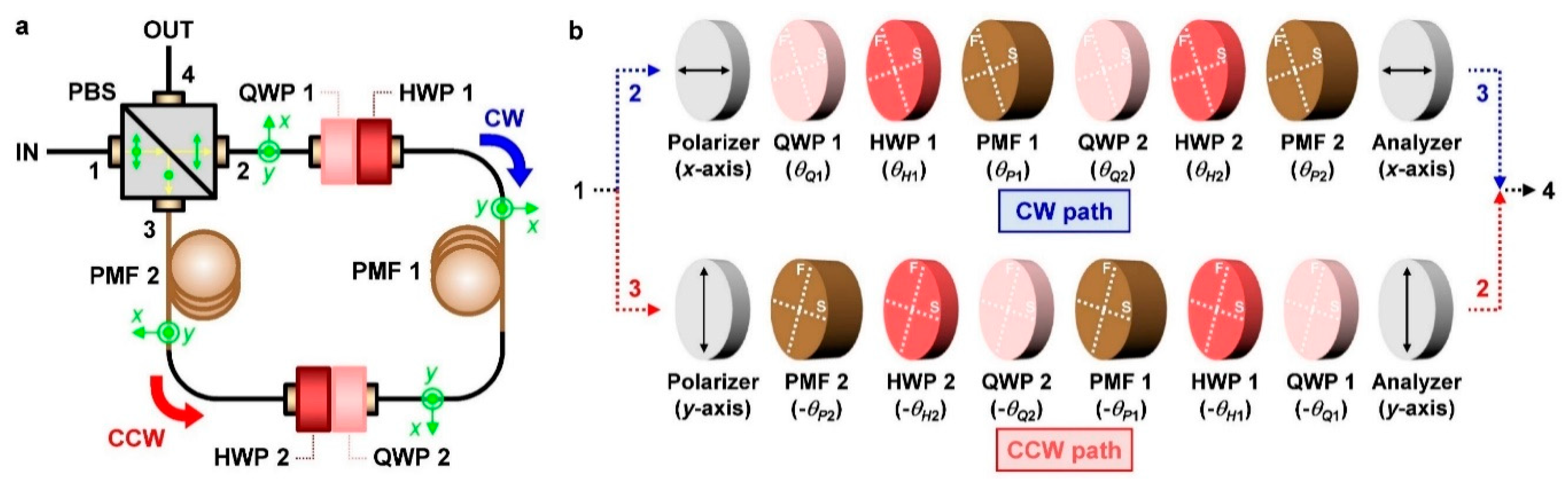
Figure 1a shows a schematic diagram of the proposed comb filter comprised of a PBS, two PMF segments whose lengths are equal (denoted by PMF 1 and PMF 2), two QWPs (denoted by QWP 1 and QWP 2), and two HWPs (denoted by HWP 1 and HWP 2). As shown in Figure 1a, one OWS of QWP 1 and HWP 1 is placed ahead of PMF 1, and the other OWS of QWP 2 and HWP 2 is located between PMF 1 and PMF 2. Every OWS can effectively change the phase delay difference between two principal modes of the individual PMF segment, and the combination of QWP 2 and HWP 2, or the second OWS, has an additional function to effectively modify the relative angular difference between the principal axes of PMF 1 and PMF 2. The slow axis of PMF 2 butt-coupled to port 3 of the PBS is 22.5° away from the TM polarization axis (denoted by x axis) of the PBS. An input beam introduced into port IN of the filter is decomposed into two orthogonal linear polarization components, such as linear horizontal polarization (LHP) and linear vertical polarization (LVP), which circulate through the polarization-diversified loop of the filter in the clockwise (CW) and counterclockwise (CCW) directions, respectively. Figure 1b shows the two propagation paths of light travelling through the filter, designated as CW and CCW paths. When the SOP_in of the filter is LHP, input light propagates along the CW path and sequentially passes through a linear horizontal polarizer (x axis), QWP 1 (with its slow axis oriented at θ_Q1 for the x axis), HWP 1 (oriented at θ_H1), PMF 1 (oriented at θ_P1), QWP 2 (oriented at θ_Q2), HWP 2 (oriented at θ_H2), PMF 2 (oriented at θ_P2 = 22.5°), and a linear horizontal analyzer (x axis). In the case of the SOP_in of LVP, input light propagates through a linear vertical polarizer (y axis), PMF 2 (−θ_P2 oriented), HWP 2 (−θ_H2 oriented), QWP 2 (−θ_Q2 oriented), PMF 1 (−θ_P1 oriented), HWP 1 (−θ_H1 oriented), QWP 1 (−θ_Q1 oriented), and a linear vertical analyzer (y axis) in turn, circulating along the CCW path. F and S displayed on the waveplates and the PMFs indicate their fast and slow axes, respectively.

Polarization interference is created by optical birefringence in an optical structure composed of two linear polarizers and BEs inserted between them. In the case of one BE like a PMF segment, the transmittance function of this optical structure becomes a sinusoidally varying function of Γ, the phase delay difference between two principal modes of the BE, which is represented by 2πBL/λ, where B, L, and λ are the birefringence of the BE, the length of the BE, and the free space wavelength, respectively. It is possible to tune the wavelength of this polarization interference spectrum by modifying Γ, and the modification of Γ can be done by adding a supplementary phase delay difference ϕ to Γ and modulating this ϕ [21]. In the same way, to tune the wavelength position of the first-order comb spectrum generated with two BEs, or two PMF segments [26], ϕ, which is added to Γ for individual PMF, should be modulated equally for both PMF 1 and PMF 2. This simultaneous ϕ modulation can be accomplished by changing the SOP_in‘s of PMF 1 and PMF 2 with two OWS’s. When we increase ϕ from 0° to 360° by appropriately adjusting the SOP_in of each PMF, the comb spectrum makes a redshift by an interference period, i.e., a free spectral range (FSR). The filter transmittance function t_filter can be derived from the Jones transfer matrix [27] T given by (1) and is represented as (2). In this derivation, no insertion losses are assumed to exist in any optical components of the filter, and all waveplates are regarded as wavelength-independent.

$$\begin{gathered} \begin{array}{c}T=\left[\begin{array}{cc}1& 0\\ 0& 0\end{array}\right]T_{PMF2}\left({\theta }_{P2}\right)T_{HWP2}\left({\theta }_{H2}\right)T_{QWP2}\left({\theta }_{Q2}\right)T_{PMF1}\left({\theta }_{P1}\right)T_{HWP1}\left({\theta }_{H1}\right)T_{QWP1}\left({\theta }_{Q1}\right)\left[\begin{array}{cc}1& 0\\ 0& 0\end{array}\right]\\ +\left[\begin{array}{cc}0& 0\\ 0& 1\end{array}\right]T_{QWP1}\left(-{\theta }_{Q1}\right)T_{HWP1}\left(-{\theta }_{H1}\right)T_{PMF1}\left(-{\theta }_{P1}\right)\times \\ \\ T_{QWP2}\left(-{\theta }_{Q2}\right)T_{HWP2}\left(-{\theta }_{H2}\right)T_{PMF2}\left(-{\theta }_{P2}\right)\left[\begin{array}{cc}0& 0\\ 0& 1\end{array}\right]\end{array} \end{gathered}$$

(1)

$$t_{filter}=\frac{1}{4}{\left(P_0+P_1\cos \Gamma +P_2\sin \Gamma \right)}^2+\frac{1}{4}{\left(Q_0+Q_1\cos \Gamma +Q_2\sin \Gamma \right)}^2$$

(2)

Here, T_QWP1, T_HWP1, T_PMF1, T_QWP2, T_HWP2, and T_PMF2 mean the transfer matrices of QWP 1, HWP 1, PMF 1, QWP 2, HWP 2, and PMF 2, whose slow-axis orientation angles are θ_Q1, θ_H1, θ_P1, θ_Q2, θ_H2, and θ_P2 (given by 22.5° here) for the x axis, respectively. P₀ = −sinαsinβ − sin(γ − π/4)sin(δ − 2θ_P1), Q₀ = cosγcosβ − cos(α − π/4)cos(δ − 2θ_P1), P₁ = −sinαsinβ + sin(γ − π/4)sin(δ − 2θ_P1), Q₁ = cosγcosβ + cos(α − π/4)cos(δ − 2θ_P1), P₂ = cos(γ − π/4)cosβ + cosαcos(δ − 2θ_P1), and Q₂ = sin(α − π/4)sinβ − sinγsin(δ − 2θ_P1), where α = 2θ_H2 − (θ_Q1 + θ_Q2), β = 2θ_H1 − (θ_Q1 + θ_Q2), γ = 2θ_H2 + (θ_Q1 − θ_Q2), and δ = 2θ_H1 − (θ_Q1 − θ_Q2).

Before we begin to address the principle of the phase modulation of a GTF, let us consider the previous conclusions on the relationship between SOP changes and the continuous wavelength tuning of a narrowband transmittance t_n given by (3) in the comb filter composed of two PMF segments, two OWS’s of an HWP and a QWP, and the third HWP. [23,24].

$$t_n=\left[3-4\cos \left(\Gamma +\varphi \right)+\cos 2\left(\Gamma +\varphi \right)\right]/8$$

(3)

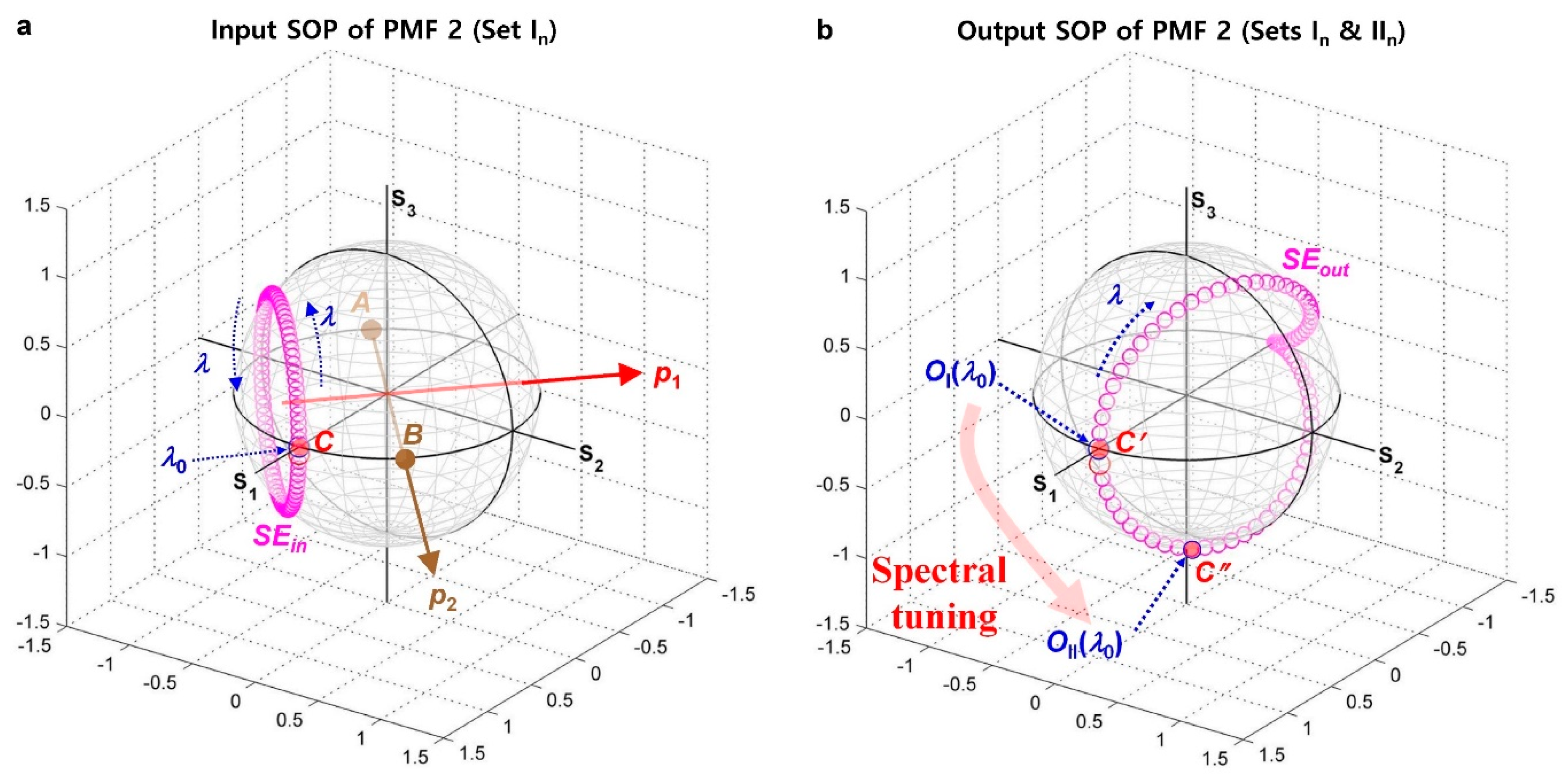
The additional phase delay difference ϕ in (3) defines the absolute wavelength position of the narrowband transmission spectrum. In the previous studies [23,24], eight WOA sets (from Set I_n to Set VIII_n) of four waveplates (except for the third HWP) were utilized to display eight wavelength-tuned spectra calculated from t_n with eight ϕ values from 0° to 315° (increment: 45°). When the wavelength of input light increases from λ₀ to λ₀ + ∆λ, where ∆λ implies the FSR, the SOP_in of PMF 2 at Set I_n (ϕ = 0°) spectrally evolves on the Poincare sphere, as shown in Figure 2a. This spectral evolution indicated by pink circles is denoted by SE_in. With increasing wavelength, the SOP_in moves along the SE_in trace rotating CW around the normal vector p₁, when p₁ points the observer. The rotation direction of the SOP_in can also be thought using a left-hand rule. If the direction of p₁ is the same as that of the left thumb, the direction of the rest of the fingers is the rotation direction of the SOP_in with the increase of the wavelength. In general, the SOP_out of the birefringent medium rotates around its slow axis on the Poincare sphere according to the wavelength λ of light passing through the medium. The vector AB connecting A (2ε = 0°, 2ψ = −135°) and B (2ε = 0°, 2ψ = 45°), which lie on the Poincare sphere, points the direction of the slow axis of PMF 2 (θ_P2 = 22.5°) and is denoted by the vector p₂. Here, 2ε (−90° ≤ 2ε ≤ 90°) and 2ψ (−180° ≤ 2ψ ≤ 180°) are the latitude and longitude of the Poincare sphere, respectively. For convenience, the plane whose normal vector is p₁, that is, the plane of the SE_in trace, is designated as the SOP_in plane, and another plane with its normal vector of p₂ is designated as the SOP_out plane. Actually, p₂ is an axis of revolution, around which the SE_in trace moves as ϕ varies. Hence, p₁ and the SOP_out plane are parallel, and p₂ and the SOP_in plane are parallel, ending up with p₁ and p₂ being perpendicular. At Set II_n (ϕ = 45°), the SE_in trace shown in Figure 2a rotates CCW by 45° around both p₁ and p₂, and thus p₁ shown in Figure 2a rotates 45° CCW about p₂ as well. Analogously, for the remaining six sets (III_n–VIII_n), the SE_in trace at Set I_n rotates CCW by 90°–315° (with an increment of 45°) around both p₁ and p₂.

Likewise, the SOP_out’s of PMF 2 at Sets I_n (ϕ = 0°) and II_n (ϕ = 45°) spectrally evolve on the Poincare sphere over the same wavelength range of λ₀ to λ₀ + ∆λ, as shown in Figure 2b. This spectral evolution also indicated by pink circles is designated as SE_out. This SE_out trace is embodied by making a CW rotation of the wavelength-dependent SOP_in of PMF 2 about p₂ by an angle φ(λ) given by 360°(λ − λ₀)/∆λ. When PMF 2 is passed through by light at λ₀, the SOP_in of PMF 2 at λ₀, C (2ε = 0°, 2ψ = 0°) shown in Figure 2a, rotates CW around p₂ by φ(λ₀) = 0°, and the SOP_out of PMF 2 at λ₀ becomes C′ (2ε = 0°, 2ψ = 0°) shown in Figure 2b without a change in the position on the Poincare sphere. Similarly, the SOP_in of PMF 2 at λ₀ + ∆λ/4 rotates CW around p₂ by φ(λ₀ + ∆λ/4) = 90° during its passage through PMF 2. If we put the SOP_out of PMF 2 at a certain wavelength λ as O(λ), O(λ₀) at Set I_n, marked by O_I(λ₀) in the figure, becomes C′. Owing to the wavelength-dependent transformation of the SOP_in of PMF 2, O(λ) forms a non-circular trajectory SE_out shaped like a droplet as λ increases from λ₀ to λ₀ + ∆λ. During the wavelength increase of ∆λ starting from λ₀, O(λ) goes round this entire SE_out trace starting from C′ in the CW direction around the S₂ axis. If we assume the wavelength at which t_n is maximized as λ_peak, λ_peak can be regarded as λ₀ at Set I_n because t_n reaches the maximum when O(λ) is nearest to LHP (2ε = 0°, 2ψ = 0°) on the Poincare sphere. At Set II_n, O_II(λ₀), i.e., the SOP_out of PMF 2 at λ₀, becomes C′′ distant from O_I(λ₀) by an angular displacement that corresponds to ∆λ/8 and also goes round the entire SE_out trace starting from C′′ about the S₂ axis in the CW direction, as the wavelength increases from λ₀ to λ₀ + ∆λ. Here, O_I(λ₀) or O_II(λ₀) is the initial point of the spectral evolution of O(λ). The position difference between O_I(λ₀) and O_II(λ₀) originates from the fact that, while the WOA set goes from Set I_n to Set II_n, the SE_in trace at Set I_n is rotated CCW by 45° not only about p₁ on the SOP_in plane but also about p₂ on the SOP_out plane. This means that simultaneously rotating the SE_in trace CCW about both p₁ and p₂ can change the position of O(λ₀) along the SE_out trace. On the SE_out trace at Set II_n, therefore, O_II(λ₀ + ∆λ/8) is located at C′, and λ₀ + ∆λ/8 becomes λ_peak because C′ is nearest to LHP. This implies that the narrowband transmission spectrum moves towards a longer wavelength region by ∆λ/8, that is, ϕ is modulated by 45° making t_n be redshifted by (45°/360°)∆λ = ∆λ/8. Similarly, for remaining Sets III_n–VIII_n, ϕ is modulated by 90° to 315° with an increment of 45° making t_n be redshifted by ∆λ/4 to 7∆λ/8 with a step of ∆λ/8, and λ_peak changes from λ₀ + ∆λ/4 to λ₀ + 7∆λ/8 with an increment of ∆λ/8.

In the case of a GTF, or an arbitrary transmittance function, obtained in the proposed filter structure, the SOP_out trace of PMF 2, designated as SE_out,GTF trace, is presumed to be a completely different trajectory in comparison with the SE_out trace shown in Figure 2b. However, it can be deduced from the aforementioned conclusions of the previous works that a location change of O(λ₀) along the SE_out,GTF trace, accompanied by a shift in λ_peak, is responsible for a phase modulation in the GTF, resulting in a wavelength shift in the transmission spectrum. For a given SE_out,GTF trace, the corresponding SOP_in trace of PMF 2, designated as SE_in,GTF trace, should be a circle on the Poincare sphere as well, since a wavelength-dependent BE through which light has passed is just one, PMF 1. However, in terms of the radius and the normal vector (p₁) of the circular trace, this SE_in,GTF trace will be quite different from the SE_in trace shown in Figure 2a. Because it is assumed that all waveplates used here are independent of wavelength, they do not distort the shape of the SOP_in or the SOP_out trace. Thus, the SOP_out trace of PMF 1 also has a circular shape identical to that of the SE_in,GTF trace. Like the relationship between the SE_in and SE_out traces, the increase in λ_peak results from the CCW revolution of the SE_in,GTF trace about both p₁ on the SOP_in plane and p₂on the SOP_out plane. If the SE_in,GTF trace is revolved CCW about both p₁ and p₂ by an amount of ξ, the transmission spectrum makes a redshift of (ξ/360°)∆λ, resulting in an increase of (ξ/360°)∆λ in λ_peak. That is to say, ξ can be regarded as ϕ, or the additional phase delay difference. Thus, as ξ varies from 0° to 360°, the phase of the GTF also changes from 0° to 360°, which means that the GTF is able to be phase-modulated continuously by varying ξ. Briefly, one simultaneous CCW rotation of the SE_in,GTF trace about both p₁ and p₂, implemented by controlling four waveplates contained within the proposed filter, enables its transmission spectrum to be redshifted by an FSR (∆λ), in other words, its phase to be modulated by 360°.

3. Finding Algorithm of Waveplate Orientation Angles (WOA’s) for Phase Modulation of General Transmittance Function (GTF)

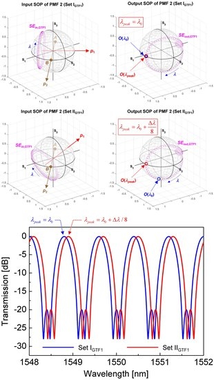
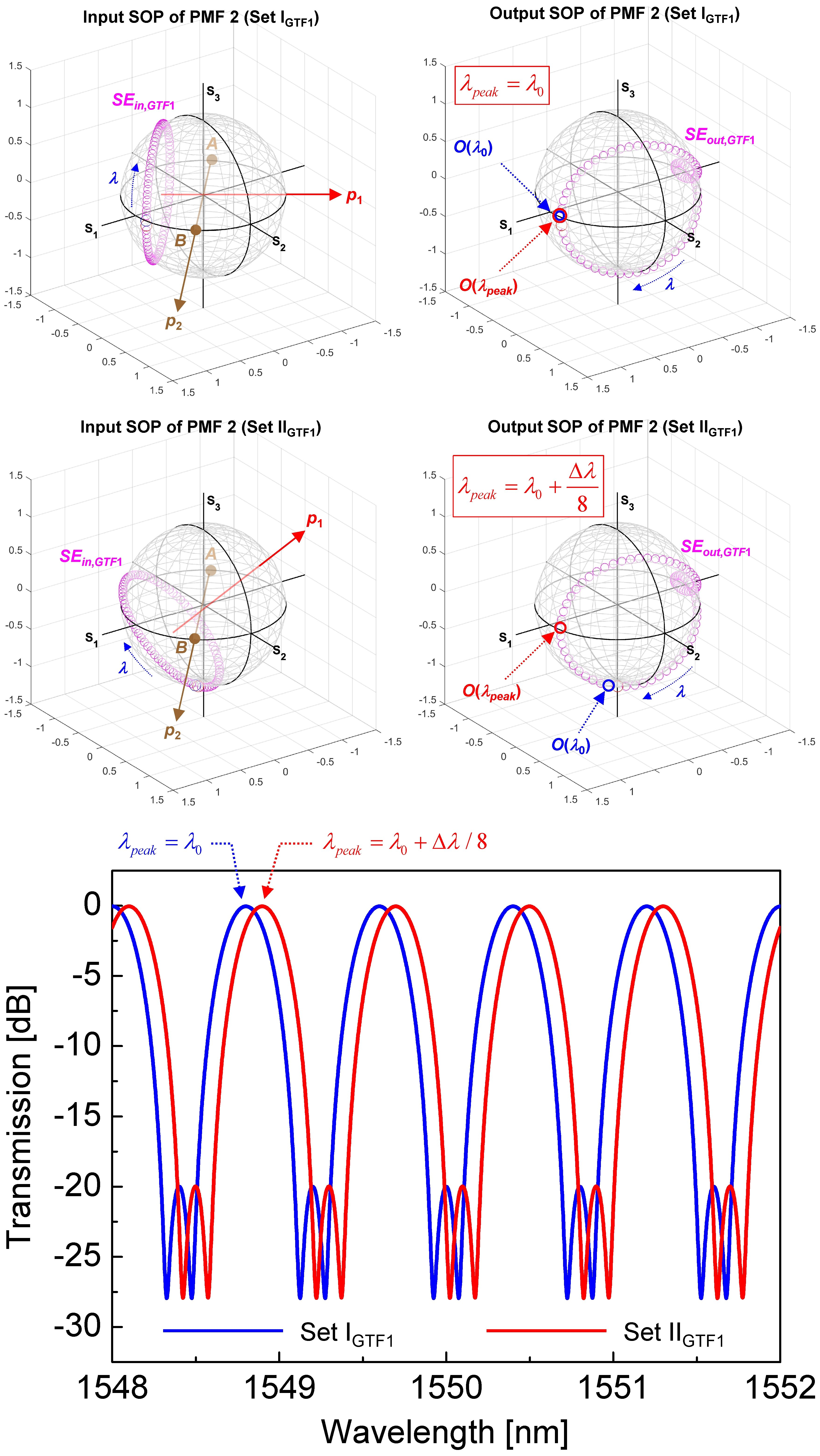
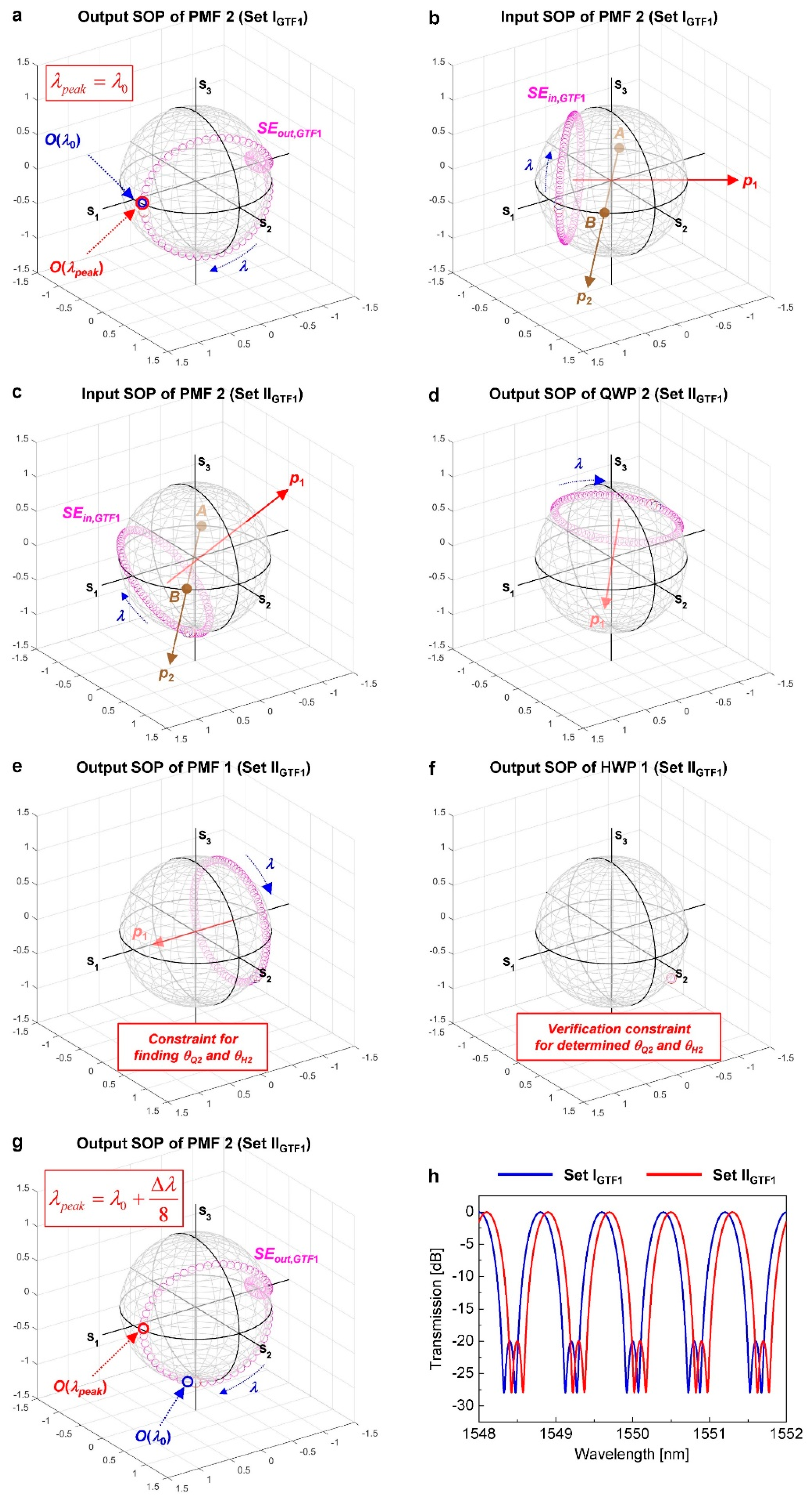
Considering the aforementioned polarization conditions required for arbitrarily modulating the phase of a GTF or continuously tuning its wavelength, the WOA’s (θ_Q1, θ_H1, θ_Q2, θ_H2) for this arbitrary phase modulation (i.e., continuous wavelength tuning) are investigated with our unique WOA-finding algorithm. This algorithm is suggested as it is quite sophisticated to draw out an exact mathematical expression of a GTF having an application-specific unique spectrum. Moreover, although the mathematical expression t_GTF of a GTF is given, it is cumbersome to solve (θ_Q1, θ_H1, θ_Q2, θ_H2) from trigonometric simultaneous equations obtained from direct comparison of t_GTF with t_filter in (2). To explain our angle-finding approach, let us choose a specific GTF t_GTF1, which is procured at a certain selected WOA set (θ_Q1, θ_H1, θ_Q2, θ_H2) = (118.23°, 149.56°, 179.42°, 123.46°), and find (θ_Q1, θ_H1, θ_Q2, θ_H2) where t_GTF1 is wavelength-tuned. At the above selected WOA set indicated by Set I_GTF1 and fixed orientation angles of PMF 1 and PMF 2 (θ_P1 = 0° and θ_P2 = 22.5°), the SOP_out trace of PMF 2, or SE_out,GTF1, is obtained over a wavelength range from λ₀ (=1548.0 nm) to λ₀ + ∆λ (=0.8 nm), as shown in Figure 3a. At Set I_GTF1, O(λ₀) indicated in Figure 3a is located nearest to LHP on the Poincare sphere, which makes the filter transmittance be maximized at λ₀. If we put the wavelength at which t_GTF1 is maximized as λ_peak, O(λ₀) becomes O(λ_peak), that is, λ_peak = λ₀ = 1548.0 nm at Set I_GTF1. The SOP_in trace of PMF 2, or SE_in,GTF1 in Figure 3b, can be derived by utilizing the inverse matrix of T_PMF2 (T_PMF2⁻¹) and the SE_out,GTF1 trace in Figure 3a. Based on the foregoing description on the phase modulation of the GTF using the SE_in,GTF and SE_out,GTF traces, another SE_in,GTF1 trace shown in Figure 3c can be obtained by rotating the SE_in,GTF1 trace at Set I_GTF1 CCW by 45° around both p₁ and p₂, for the phase modulation of 45° (i.e., the wavelength tuning of ∆λ/8 = 0.1 nm) in t_GTF1. It is easily expected that this new SE_in,GTF1 trace will be obtained at another WOA set (θ_Q1, θ_H1, θ_Q2, θ_H2) designated later as Set II_GTF1.

What we should focus on is a way to obtain Set II_GTF1, another WOA set described above. Basically, the SOP_out of one component of the filter is equivalent to the SOP_in of the following component in any propagation path shown in Figure 1b. As our discussion is confined to the CW path, as an example, the SOP_out of PMF 1 is equivalent to the SOP_in of QWP 2. The same thing can be said for SOP traces. For example, the SOP_in trace of HWP 1 is the same as the SOP_out trace of QWP 1. A QWP and an HWP rotate input polarization CCW by 90° and 180° about their slow axes on the Poincare sphere, respectively. If an SOP trace, composed of multiple different SOP’s distributed on the Poincare sphere, enters a waveplate, therefore, not its shape but its position is altered by the waveplate. For a given SE_in,GTF1 trace at Set II_GTF1 (in Figure 3c), a certain SOP_out trace of QWP 2 can be obtained by using the SE_in,GTF1 trace (i.e., the SOP_out trace of HWP 2) and the inverse matrix of T_HWP2, or T_HWP2⁻¹, if θ_H2 is fixed as one value (unknown yet). With this SOP_out trace of QWP 2, shown in Figure 3d, a corresponding SOP_out trace of PMF 1, which is transformed into the SOP_out trace of QWP 2 after passing through QWP 2, can also be derived similarly by using the predetermined SOP_out trace of QWP 2 and T_QWP2⁻¹, if θ_Q2 is fixed as another value (unknown either), as shown in Figure 3e. Because the SOP rotation due to a QWP or an HWP applies equally to all points comprising an SOP trace, the shape of the SOP trace created by PMF 1 remains the same after passage through HWP 2 or QWP 2, and thus the trajectory shape of the SOP_out trace of QWP 2 or PMF 1 is equal to that of the SE_in,GTF1 trace. In terms of the SOP_out trace of PMF 1, however, p₁, the normal vector of the trace, coincides with the S₁ axis on the Poincare sphere as the orientation angle θ_P1 of PMF 1 is 0°, as shown in Figure 3e. Then, θ_H2 and θ_Q2 can be determined by finding the SOP_out trace of PMF 1 to satisfy this constraint for p₁.

After both θ_H2 and θ_Q2 are elucidated, the SOP_out of HWP 1, which is displayed as an SOP location on the Poincare sphere, can simply be determined using the SOP_out trace of PMF 1 and T_PMF1⁻¹, as shown in Figure 3f. In particular, the validity of θ_H2 and θ_Q2 determined above can be verified by checking whether this SOP_in of PMF 1 is a single SOP point or not. That is to say, if θ_H2 and θ_Q2 predetermined abiding by the above constraint for p₁ are suitable for the WOA set at Set II_GTF1, the SOP_in of PMF 1 should be unchanged even with variations in the wavelength from λ₀ to λ₀ + ∆λ. As θ_H2 and θ_Q2 are found from the SE_in,GTF1 trace at Set II_GTF1, this SOP_in of PMF 1 (i.e., the SOP_out of HWP 1) is the starting point to unveil θ_H1 and θ_Q1. By using the SOP_out of HWP 1 (in Figure 3f) and T_HWP1⁻¹, the SOP_out of QWP 1 can be obtained, if we set θ_H1 as a fixed value (unknown yet). Moreover, for a fixed value (unknown either) of θ_Q1, a corresponding SOP_in of QWP 1 can be drawn out from the above SOP_out of QWP 1 and T_QWP1⁻¹. Then, to find θ_H1 andθ_Q1, we can harness the fundamental SOP constraint that the SOP_in of QWP 1 should be LHP because light emerging from port 2 of the PBS is linear horizontally polarized. Through this reverse tracing algorithm described above, (θ_Q1, θ_H1, θ_Q2, θ_H2) at Set II_GTF1 could be found to be (108.49°, 132.67°, 201.92°, 134.71°), and it was also confirmed from additional calculations, although not suggested here, that several degenerate WOA sets could also exist for t_GTF1 at Set II_GTF1. It is figured out from the SOP_out trace of PMF 2 at Set II_GTF1, the SE_out,GTF1 trace in Figure 3g, that O(λ₀) at Set II_GTF1 differs from O(λ₀) at Set I_GTF1, although the shape of the SE_out,GTF1 trace at Set II_GTF1 remains unchanged in comparison with the shape of the SE_out,GTF1 trace at Set I_GTF1. From O(λ₀) at Set I_GTF1, O(λ₀) at Set II_GTF1 is distant by an angular displacement that corresponds to ∆λ/8 along this SE_out,GTF1 trace towards decreasing wavelength. This implies that O(λ₀ + ∆λ/8) at Set II_GTF1 is the same as O(λ₀) at Set I_GTF1 and also as O(λ_peak) at Set II_GTF1, and λ_peak becomes λ₀ + ∆λ/8 at Set II_GTF1, resulting in a wavelength shift of ∆λ/8 in t_GTF1 (i.e., a phase modulation of 45°). Figure 3h shows two transmission spectra of t_GTF1, which are calculated at Sets I_GTF1 and II_GTF1 and displayed by blue and red solid lines, respectively. It is apparent that the transmission spectrum at Set II_GTF1 is redshifted by ∆λ/8 (= 0.1 nm) compared with that at Set I_GTF1. In short, for a phase modulation of η, or a wavelength tuning of (η/360°)∆λ, in t_GTF1, one should find a new SE_in,GTF1 trace first, obtained by revolving the SE_in,GTF1 trace at Set I_GTF1 CCW by η in angle about p₁ and p₂. Then, one can find (θ_Q1, θ_H1, θ_Q2, θ_H2) for this new SE_in,GTF1 trace through the WOA-searching procedures addressed above. If we pick η within 0° to 360°, t_GTF1 can be arbitrarily phase-modulated. This arbitrary phase modulation can be utilized directly for the continuous wavelength tuning of t_GTF1.

4. WOA’s for Phase Modulation of GTF and Its Phase-Modulated Spectra

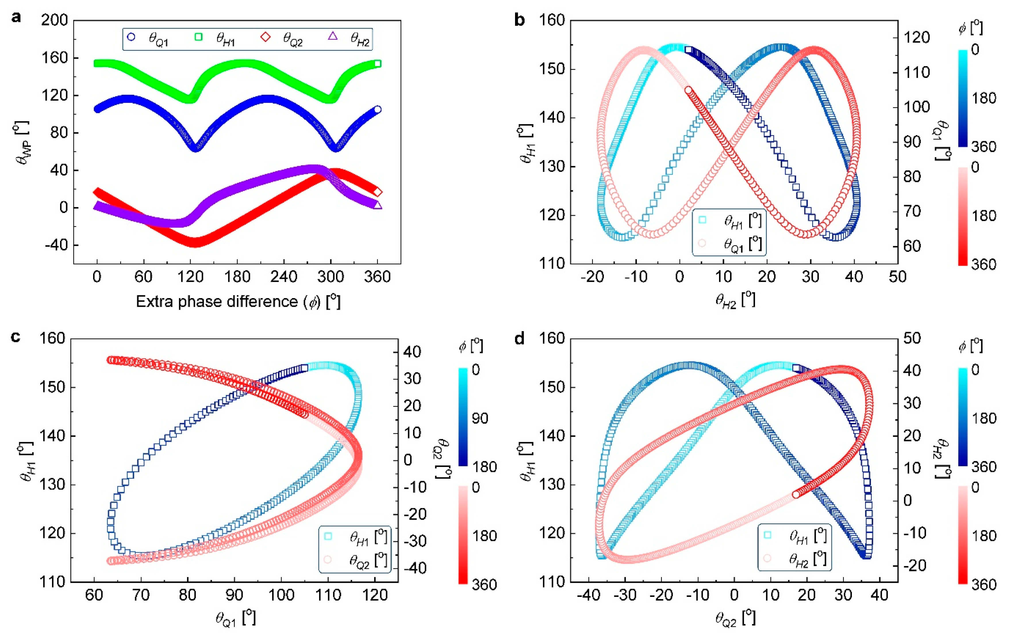
Here, we explore WOA sets for continuous phase modulation of another GTF t_GTF2, which is defined at another different (θ_Q1, θ_H1, θ_Q2, θ_H2) = (105°, 154°, 17°, 2°) with θ_P1 = 0° and θ_P2 = 22.5°, by using our reverse tracing method. Specifically, 360 sets of (θ_Q1, θ_H1, θ_Q2, θ_H2), where an additional phase shift of 1°–360° (increment: 1°) can be induced in t_GTF2, were found with our method. Figure 4a shows the 360 sets of (θ_Q1, θ_H1, θ_Q2, θ_H2) as functions of ϕ ranging from 0° to 360° (step: 1°), displayed by blue circles (θ_Q1), green squares (θ_H1), red diamonds (θ_Q2), and violet triangles (θ_H2), respectively, which are found at fixed values of θ_P1 = 0° and θ_P2 = 22.5°. In contrast with WOA sets for continuous wavelength tuning of an analytic transmittance t_n [23,24], all four WOA’s (θ_Q1, θ_H1, θ_Q2, and θ_H2) do not take the form of simple mathematical functions of ϕ and have similar patterns either. Whereas θ_Q1(ϕ) and θ_H1(ϕ) have a period of 180°, the period of θ_Q2(ϕ) or θ_H2(ϕ) is 360°. θ_Q1, θ_H1, θ_Q2, and θ_H2 are bounded in the WOA ranges of 63.5° < θ_Q1 < 116.6°, 115.4° < θ_H1 < 154.6°, −37.2° < θ_Q2 < 37.2°, and −18.1° < θ_H2 < 40.6°, respectively. In order to reveal implicit information on the 360 sets of (θ_Q1, θ_H1, θ_Q2, θ_H2) in Figure 4a, we investigated the relationship between any two of the four WOA’s. Figure 4b shows the loci of (θ_H2, θ_H1) and (θ_H2, θ_Q1), displayed by blueish squares and reddish circles, respectively. These loci were drawn using θ_H2(ϕ), θ_H1(ϕ), and θ_Q1(ϕ) in Figure 4a in the Cartesian coordinate system at a range of ϕ from 0° to 360°. As ϕ increases from 0° to 360°, (θ_H2, θ_H1) or (θ_H2, θ_Q1) forms a closed locus, whose shape is similar to a squeezed goggle or an infinity symbol, respectively. Because the period of θ_H2(ϕ) is two times longer than that of θ_H1(ϕ) or θ_Q1(ϕ), both loci have two-fold symmetry. It is readily seen that the density of the point (θ_H2, θ_H1) or (θ_H2, θ_Q1), the interval between two locus points, is different along the locus. In terms of the locus of (θ_H2, θ_H1), the lower inner part of the locus is sparser than its other parts. This implies that the ϕ variation is smaller at the lower inner part of the locus for the same amounts of changes in θ_H2 and θ_H1. Similarly, in terms of the locus of (θ_H2, θ_Q1), the upper part of the locus is denser than its lower part, which means that the ϕ variation is larger at the upper part of the locus for the same amounts of changes in θ_H2 and θ_Q1. Next, the loci of (θ_Q1, θ_H1) and (θ_Q1, θ_Q2), displayed by blueish squares and reddish circles, are plotted with θ_Q1(ϕ), θ_H1(ϕ), and θ_Q2(ϕ) in Figure 4a at ϕ ranges of 0°–180° and 0°–360°, respectively, as shown in Figure 4c. In terms of the locus of (θ_Q1, θ_H1), the point of (θ_Q1, θ_H1) makes a round along this elliptical locus from (105°, 154°) in the CW direction, while ϕ increases from 0° to 180°. It can be seen that the right side of this elliptical locus is much denser than its left side, which suggests that an equal displacement of the point (θ_Q1, θ_H1) on the locus results in a relatively greater change in ϕ at the right side. Even if the (θ_Q1, θ_H1) locus is not represented using analytic mathematical expressions as suggested in the previous work [22], the desirable phase ϕ, i.e., the desirable transmission dip (or peak) wavelength, can be set and be continuously changed by selecting and shifting (θ_Q1, θ_H1) on this locus, respectively, while letting θ_Q2 and θ_H2 follow the WOA curves of θ_Q2(ϕ) and θ_H2(ϕ) in Figure 4a, respectively. In terms of the locus of (θ_Q1, θ_Q2), the point of (θ_Q1, θ_Q2) makes a closed parabolic trace for ϕ increasing from 0° to 360°. Like the (θ_H2, θ_H1) and (θ_H2, θ_Q1) loci in Figure 4b, this (θ_Q1, θ_Q2) locus also has a two-fold symmetry with respect to the θ_Q1 axis because θ_Q2(ϕ) has a period two times longer than θ_Q1(ϕ). Moreover, the density difference on the locus is analogous to that of the (θ_Q1, θ_H1) locus. Figure 4d shows the loci of (θ_Q2, θ_H1) and (θ_Q2, θ_H2), displayed by blueish squares and reddish circles, respectively. θ_Q2(ϕ), θ_H1(ϕ), and θ_H2(ϕ) in Figure 4a are utilized to plot these loci at a ϕ range of 0°–360°. (θ_Q2, θ_H1) forms a locus shaped like inverted Spiderman’s eyes with increasing ϕ (from 0° to 360°), which also has a two-fold symmetry with respect to the θ_H1 axis owing to the period of θ_Q2(ϕ) two times longer than that of θ_H1(ϕ). It can also be found that the lower outer part of the (θ_Q2, θ_H1) locus is sparser than its other parts. The locus of (θ_Q2, θ_H2) forms a parallelogram-shaped trace, which makes one CW revolution along the locus, starting at (17°, 2°), while ϕ varies from 0° to 360°. The left and right sides of the (θ_Q2, θ_H2) locus are slightly sparser than its other parts. This indicates that an identical displacement of the point (θ_Q2, θ_H2) along the locus causes a relatively smaller modification of ϕ at these parts of the locus. In sum, it is confirmed from Figure 4 that one can always find a WOA set (θ_Q1, θ_H1, θ_Q2, θ_H2) with respect to any ϕ (increasing from 0° to 360° by 1°). This means that the phase of t_GTF2 can be continuously modulated, also indicating that t_GTF2 can be continuously frequency-tuned. As long as an initial WOA set where any GTF is obtained is given, one can always find a WOA set inducing an arbitrary phase in this GTF.

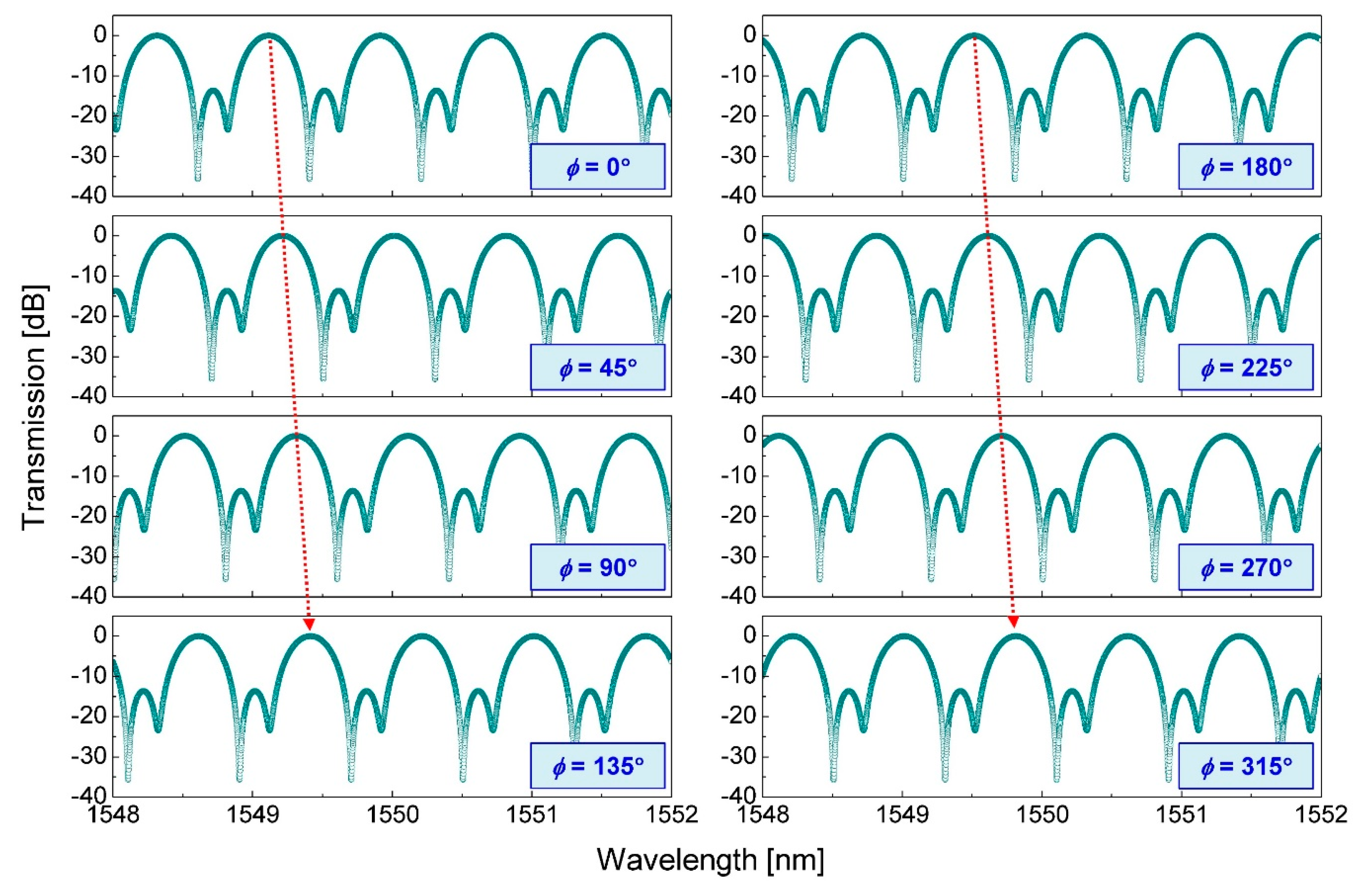
To examine if the WOA sets found by our angle-finding method can embody the predicted continuous phase modulation of t_GTF2, the transmission spectra of t_GTF2 were calculated at eight WOA sets, which were chosen from the WOA sets found above for the phase modulation of t_GTF2, with θ_P1 and θ_P2 set at 0° and 22.5°, respectively. The chosen WOA sets, denoted by Sets I_GTF2, II_GTF2, III_GTF2, IV_GTF2, V_GTF2, VI_GTF2, VII_GTF2, and VIII_GTF2, enable ϕ’s to be chosen as 0°, 45°, 90°, 135°, 180°, 225°, 270°, and 315°, respectively. The transmission spectra of the GTF t_GTF2, shown in Figure 5, were calculated at the eight WOA sets (Sets I_GTF2–VIII_GTF2) in a wavelength range of 1548–1552 nm. For the calculation of the transmission spectrum, the length L and birefringence B of PMF (PMF 1 or PMF 2) were set as 7.2 m and 4.166 × 10⁻⁴, respectively, so that ∆λ became ~0.8 nm at 1550 nm. It can be seen from the figure that the first-order comb spectrum of deformed narrow passbands makes a redshift as ϕ is modulated as 0° to 315° (increment: 45°). If the peak wavelength of one passband is designated as λ_peak,GTF at Set I_GTF2 (ϕ = 0°), one step transition in the WOA set (e.g., from Set II_GTF2 to Set III_GTF2) leads to an increase of 45° in ϕ and of 0.1 nm in λ_peak,GTF. Linear movement of λ_peak,GTF with respect to ϕ, displayed as red-dotted arrows, directly tells us that the continuous or the desired arbitrary phase modulation of t_GTF2 can be realized. These calculation results clearly manifest that t_GTF2 can be continuously wavelength-shifted within ∆λ using the WOA sets shown in Figure 4, implying the arbitrary phase modulation capability of t_GTF2 within 360°.

5. Experimental Verification of Phase-Modulated Spectra

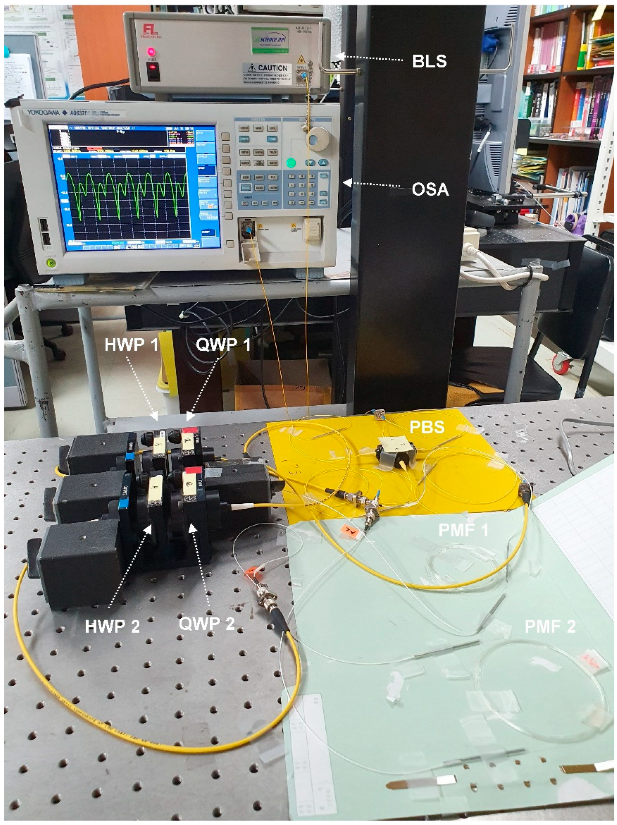
In order to verify the predicted phase modulation capability of t_GTF2 through experiments, our filter was manufactured with a fiber-pigtailed PBS (OZ Optics) with four ports, two fiber-pigtailed QWPs (OZ Optics), two fiber-pigtailed HWPs (OZ Optics), and two ~7.12 m-long segments of bow-tie PMF (Fibercore) with a birefringence of ~4.166 × 10⁻⁴, as shown in Figure 1a. Figure 6 shows an actual experimental setup for measuring the transmission spectrum of the constructed filter. As shown in Figure 6, we employed a broadband light source (BLS, Fiberlabs FL7701) covering S, C, and L bands and an optical spectrum analyzer (OSA, Yokogawa AQ6370C) to monitor the transmission spectra of the constructed filter. The input and output ports (ports 1 and 4) of the filter were connected to the BLS and OSA, respectively, with optical fiber patchcords (FC/PC type). For acquisition of high resolution and contrast optical spectra, we set the sensitivity and resolution bandwidth of the OSA as HIGH1 and 0.05 nm, respectively. To avoid unwanted position changes of all the optical components comprising the filter, we taped them up on the optical table so that they were immobilized during the spectrum measurement.

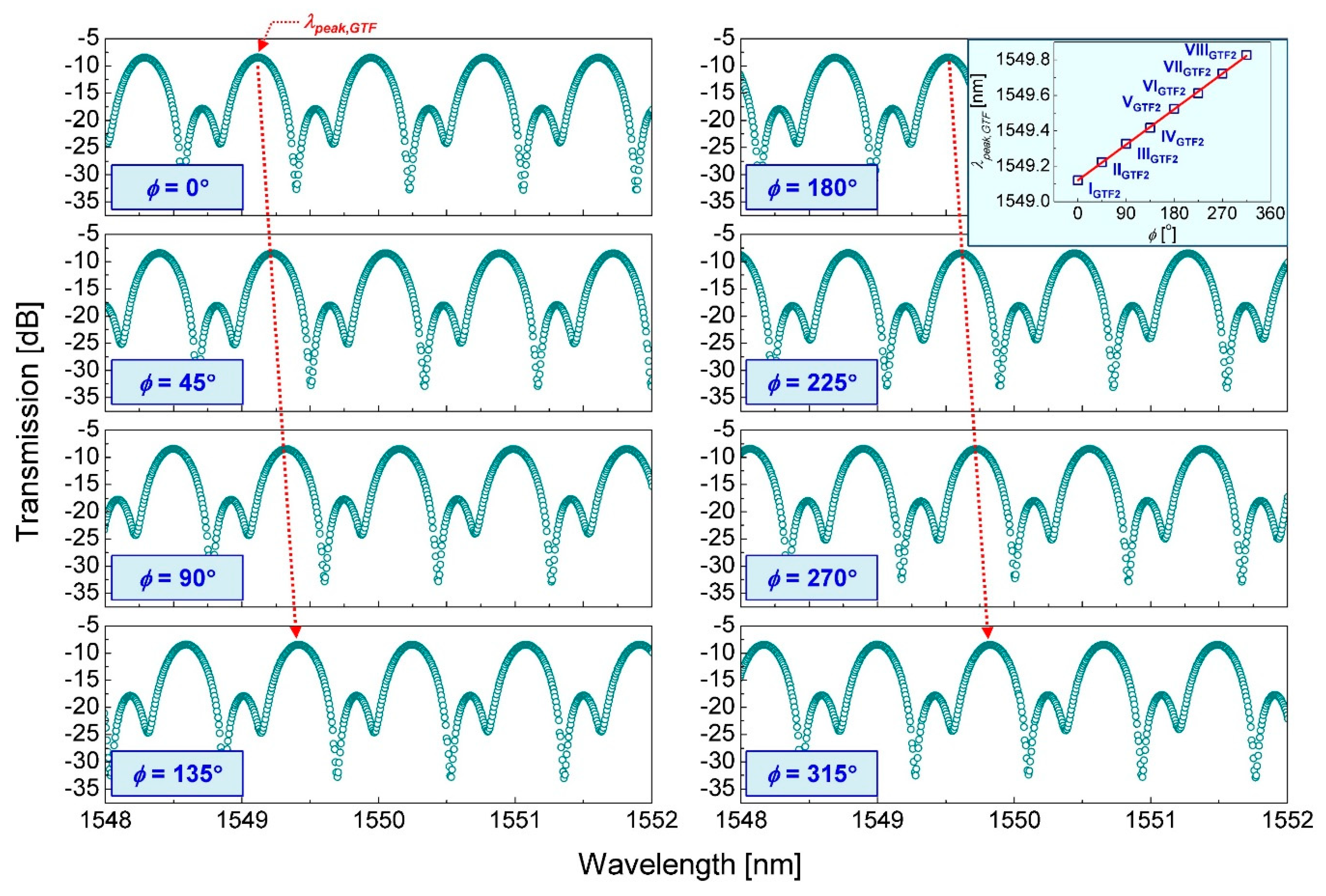
The transmission spectra of the GTF t_GTF2, shown in Figure 7, were measured at the eight WOA sets (Sets I_GTF2–VIII_GTF2) in a wavelength range of 1548–1552 nm. From the measured spectra, the FSR of the constructed filter was evaluated as ~0.8 nm around 1550 nm. This FSR is determined by L (~7.12 m) and B (~4.166 × 10⁻⁴) of PMF used here and increases with wavelength. As confirmed from the theoretical spectra in Figure 5, while the WOA set is switched from Set I_GTF2 (ϕ = 0°) to Set VIII_GTF2 (ϕ = 315°), the comb spectrum of deformed narrow passbands, which seems to be analogous to the comb spectrum shown in Figure 5, shifts towards a longer wavelength region step by step by ~0.1 nm, resulting in a total wavelength displacement of ~0.7 nm. The inset shows the variation of λ_peak,GTF (indicated as a red-dotted arrow) according to eight values of ϕ, i.e., 0°, 45°, 90°, 135°, 180°, 225°, 270°, and 315°, which are obtained at Sets I_GTF2, II_GTF2, III_GTF2, IV_GTF2, V_GTF2, VI_GTF2, VII_GTF2, and VIII_GTF2, respectively. Blue squares designated as I_GTF2–VIII_GTF2 indicate the λ_peak,GTF positions of transmission spectra obtained at eight Sets I_GTF2–VIII_GTF2. It can be figured out from the inset that λ_peak,GTF very linearly increases with ϕ showing an adjusted R² value of ~0.99946 and the tuning of the spectrum wavelength can be mediated by the phase modulation. In particular, through additional experiments, continuous frequency tuning capability was confirmed with respect to numerous ϕ values arbitrarily selected from 0° to 360° except integer multiples of 45° as well. Thus, it is experimentally verified that the GTF t_GTF2 can be arbitrarily phase-modulated by properly controlling (θ_Q1, θ_H1, θ_Q2, θ_H2), specifically, appropriately selecting (θ_Q1, θ_H1, θ_Q2, θ_H2) that satisfies the WOA sets suggested in Figure 4. Ultimately, we conclude that any GTF generated in the proposed comb filter can be phase-modulated, or wavelength-tuned, continuously by taking advantage of WOA sets that can always be drawn out with our reverse tracing algorithm.

6. Conclusions

We demonstrated the arbitrary phase modulation of a GTF, which could be obtained in the first-order fiber comb filter based on the PDLS. The proposed filter was composed of a PBS, two OWS’s of an HWP and a QWP, and two PMF segments. Each OWS was located before each PMF segment, and the second PMF segment was butt-coupled to one port of the PBS so that its principal axis should be 22.5° away from the TM polarization axis of the PBS. Basically, polarization conditions, which should be satisfied to modify the phase of a GTF as a desired value, were explained using the spectral evolution of the SOP_in and SOP_out of the second PMF in the narrowband transmittance function (t_n), on the basis of the continuous wavelength tuning mechanism of previously reported PDLS-based first-order narrowband comb filters. Then, we explained a systematic scheme to find four WOA’s for the arbitrary phase modulation of a GTF using the effect of each component of the filter, such as a waveplate or PMF segment, on its SOP_in or SOP_out. By exploiting this WOA finding method, we derived WOA sets of the four waveplates, which could give arbitrary phase delays ϕ’s from 0° to 360° to a GTF chosen here arbitrarily. Finally, we showed phase-modulated GTF’s calculated at eight selected WOA sets allowing ϕ’s to be 0°, 45°, 90°, 135°, 180°, 225°, 270°, and 315°, and then the theoretically predicted results were experimentally verified. It is concluded from the theoretical and experimental demonstrations that the GTF of our filter based on the OWS of a QWP and an HWP can be arbitrarily phase-modulated by appropriately controlling the WOA’s of the four waveplates. Our demonstration is expected to be beneficial to fiber-optic applications, which demand frequency-tunable comb filters with specific transmittances, such as microwave photonic signal processing, optical sensor interrogation, and multiwavelength lasing.

References

- Li, J.; Xu, K.; Fu, S.; Tang, M.; Shum, P.; Wu, J.; Lin, J. Photonic polarity-switchable ultra-wideband pulse generation using a tunable Sagnac interferometer comb filter. IEEE Photonics Technol. Lett. 2008, 20, 1320–1322. [Google Scholar] [CrossRef]
- Nguimdo, R.M.; Verschaffelt, G.; Danckaert, J.; Van der Sande, G. Fast photonic information processing using semiconductor lasers with delayed optical feedback: Role of phase dynamics. Opt. Express 2014, 22, 8672–8686. [Google Scholar] [CrossRef]
- Lacava, C.; Ettabib, M.; Petropoulos, P. Nonlinear silicon photonic signal processing devices for future optical networks. Appl. Sci. 2017, 7, 103. [Google Scholar] [CrossRef]
- Bian, S.Y.; Ren, M.Q.; Wei, L. A wavelength spacing switchable and tunable high-birefringence fiber loop mirror filter. Microw. Opt. Technol. Lett. 2014, 56, 1666–1670. [Google Scholar] [CrossRef]
- Ge, J.; Fok, M.P. Passband switchable microwave photonic multiband filter. Sci. Rep. 2015, 5, 15882. [Google Scholar] [CrossRef] [Green Version]
- Guo, J.-J.; Yang, Y.; Peng, G.-D. Analysis of polarization-independent tunable optical comb filter by cascading MZI and phase modulating Sagnac loop. Opt. Commun. 2011, 284, 5144–5147. [Google Scholar] [CrossRef]
- Luo, Z.-C.; Cao, W.-J.; Luo, A.-P.; Xu, W.-C. Polarization-independent, multifunctional all-fiber comb filter using variable ratio coupler-based Mach–Zehnder interferometer. J. Lightwave Technol. 2012, 30, 1857–1862. [Google Scholar] [CrossRef]
- Sun, G.; Moon, D.S.; Lin, A.; Han, W.T.; Chung, Y. Tunable multiwavelength fiber laser using a comb filter based on erbium-ytterbium co-doped polarization maintaining fiber loop mirror. Opt. Express 2008, 16, 3652–3658. [Google Scholar] [CrossRef] [Green Version]
- Pottiez, O.; Ibarra-Escamilla, B.; Kuzin, E.A.; Grajales-Coutino, R.; Gonzalez-Garcia, A. Tunable Sagnac comb filter including two wave retarders. Opt. Laser Technol. 2010, 42, 403–408. [Google Scholar] [CrossRef]
- Sova, R.M.; Kim, C.S.; Kang, J.U. Tunable dual-wavelength all-PM fiber ring laser. IEEE Photonics Technol. Lett. 2002, 14, 287–289. [Google Scholar] [CrossRef]
- Luo, Z.-C.; Luo, A.-P.; Xu, W.-C.; Yin, H.-S.; Liu, J.-R.; Ye, Q.; Fang, Z.-J. Tunable multiwavelength passively mode-locked fiber ring laser using intracavity birefringence-induced comb filter. IEEE Photonics J. 2010, 2, 571–577. [Google Scholar] [CrossRef]
- Lee, Y.W.; Han, K.J.; Lee, B.; Jung, J. Polarization-independent all-fiber multiwavelength-switchable filter based on a polarization-diversity loop configuration. Opt. Express 2003, 11, 3359–3364. [Google Scholar] [CrossRef]
- Lee, Y.W.; Han, K.J.; Jung, J.; Lee, B. Polarization-independent tunable fiber comb filter. IEEE Photonics Technol. Lett. 2004, 16, 2066–2068. [Google Scholar] [CrossRef]
- Roh, S.; Chung, S.; Lee, Y.W.; Yoon, I.; Lee, B. Channel-spacing-and wavelength-tunable multiwavelength fiber ring laser using semiconductor optical amplifier. IEEE Photonics Technol. Lett. 2006, 18, 2302–2304. [Google Scholar] [CrossRef]
- Yoon, I.; Lee, Y.W.; Jung, J.; Lee, B. Tunable multiwavelength fiber laser employing a comb filter based on a polarization-diversity loop configuration. J. Lightwave Technol. 2006, 24, 1805–1811. [Google Scholar] [CrossRef]
- Lee, Y.W.; Kim, H.-T.; Jung, J.; Lee, B. Wavelength-switchable flat-top fiber comb filter based on a Solc type birefringence combination. Opt. Express 2005, 13, 1039–1048. [Google Scholar] [CrossRef]
- Lee, Y.W.; Kim, H.-T.; Lee, Y.W. Second-order all-fiber comb filter based on polarization-diversity loop configuration. Opt. Express 2008, 16, 3871–3876. [Google Scholar] [CrossRef]
- Jo, S.; Kim, Y.; Lee, Y.W. Study on transmission and output polarization characteristics of a first-order Lyot-type fiber comb filter using polarization-diversity loop. IEEE Photonics J. 2015, 7, 1–15. [Google Scholar] [CrossRef]
- Park, K.; Lee, Y.W. Zeroth-and first-order-convertible fiber interleaving filter. IEEE Photonics J. 2016, 8, 1–10. [Google Scholar] [CrossRef]
- Park, K.; Choi, S.; Lee, S.-L.; Jeong, J.H.; Jeong, S.J.; Christian, N.J.; Kim, M.S.; Kim, J.; Kang, H.W.; Nam, S.Y.; et al. Second-order fiber interleaving filter based on polarization-diversified loop. Opt. Eng. 2017, 56, 066108. [Google Scholar] [CrossRef]
- Jung, J.; Lee, Y.W. Tunable fiber comb filter based on simple waveplate combination and polarization-diversified loop. Opt. Laser Technol. 2017, 91, 63–70. [Google Scholar] [CrossRef]
- Jung, J.; Lee, Y.W. Continuously wavelength-tunable passband-flattened fiber comb filter based on polarization-diversified loop structure. Sci. Rep. 2017, 7, 8311. [Google Scholar] [CrossRef] [Green Version]
- Jung, J.; Lee, Y.W. Polarization-independent wavelength-tunable first-order fiber comb filter. IEEE Photonics J. 2019, 11, 1–15. [Google Scholar] [CrossRef]
- Kim, D.K.; Kim, J.; Lee, S.-L.; Choi, S.; Kim, M.S.; Lee, Y.W. Tunable narrowband fiber multiwavelength filter based on polarization-diversified loop structure. J. Nanosci. Nanotechnol. 2020, 20, 344–350. [Google Scholar] [CrossRef]
- Jung, J.; Lee, Y.W. Universal wavelength tuning scheme for a first-order optical fiber multiwavelength filter based on a polarization-diversified loop structure. J. Nanosci. Nanotechnol. 2020, 20, 460–469. [Google Scholar] [CrossRef]
- Fang, X.; Ji, H.; Allen, C.T.; Demarest, K.; Pelz, L. A compound high-order polarization-independent birefringence filter using Sagnac interferometers. IEEE Photonics Technol. Lett. 1997, 9, 458–460. [Google Scholar] [CrossRef]
- Jones, R.C. A new calculus for the treatment of optical systems: I. Description and discussion of the calculus. J. Opt. Soc. Am. 1941, 31, 488–493. [Google Scholar]
Figure 1.
(a) Schematic diagram of the PDLS-based first-order fiber comb filter and (b) propagation path of light travelling through the filter.
Figure 2.
(a) Poincare sphere representation of the spectral evolution of SOPin of PMF 2 at Set In (ϕ = 0°), which is denoted by SEin (indicated by pink circles) and (b) Poincare sphere representation of the spectral evolution of SOPout of PMF 2, which is denoted by SEout (indicated by pink circles), and two O(λ0) positions at two chosen WOA sets (Sets In and IIn). All the SOP traces are obtained in the CW path of Figure 1b over a wavelength range from λ0 to λ0 + ∆λ.
Figure 3.
Wavelength-dependent variation of SOP’s in tGTF1 obtained at Set IGTF1: (a) SOPout and (b) SOPin traces of PMF 2 at Set IGTF1. Spectral evolution of SOP’s in the phase-modulated version of tGTF1, obtained at Set IIGTF1: (c) SOPin trace of PMF 2, (d) SOPout trace of QWP 2, (e) SOPout trace of PMF 1, (f) SOPout of HWP 1, and (g) SOPout trace of PMF 2. (h) Two calculated transmission spectra obtained at Sets IGTF1 and IIGTF1, indicated as blue and red solid lines, respectively.
Figure 4.
(a) Four WOA’s θQ1 (blue circles), θH1 (green squares), θQ2 (red diamonds), and θH2 (violet triangles) as a function of extra phase difference ϕ (from 0° to 360° with a step of 1°) for phase modulation of another GTF (tGTF2) at θP1 = 0° and θP2 = 22.5°. (b) Loci of (θH2, θH1) and (θH2, θQ1), displayed by blueish squares and reddish circles, respectively. (c) Loci of (θQ1, θH1) and (θQ1, θ Q2), indicated as blueish squares (ϕ: 0°–180°) and reddish circles (ϕ: 0°–360°), respectively. (d) Loci of (θQ2, θH1) and (θQ2, θH2), displayed by blueish squares and reddish circles, respectively.
Figure 5.
Calculated phase-modulated transmission spectra of GTF (tGTF2), obtained at eight WOA sets (Sets IGTF2–VIIIGTF2) where ϕ of tGTF2 is chosen as 0° to 315° with an increment of 45°.
Figure 6.
Actual experimental setup for measurement of phase-modulated transmission spectra of GTF (tGTF2).
Figure 7.
Experimental phase-modulated transmission spectra of GTF (tGTF2), measured at eight WOA sets (Sets IGTF2–VIIIGTF2).
© 2020 by the authors. Licensee MDPI, Basel, Switzerland. This article is an open access article distributed under the terms and conditions of the Creative Commons Attribution (CC BY) license (http://creativecommons.org/licenses/by/4.0/).
Share and Cite
MDPI and ACS Style
Jung, J.; Lee, Y.W. Arbitrary Phase Modulation of General Transmittance Function of First-Order Optical Comb Filter with Ordered Sets of Quarter- and Half-Wave Plates. Appl. Sci. 2020, 10, 5434. https://doi.org/10.3390/app10165434
AMA Style
Jung J, Lee YW. Arbitrary Phase Modulation of General Transmittance Function of First-Order Optical Comb Filter with Ordered Sets of Quarter- and Half-Wave Plates. Applied Sciences. 2020; 10(16):5434. https://doi.org/10.3390/app10165434
Chicago/Turabian StyleJung, Jaehoon, and Yong Wook Lee. 2020. "Arbitrary Phase Modulation of General Transmittance Function of First-Order Optical Comb Filter with Ordered Sets of Quarter- and Half-Wave Plates" Applied Sciences 10, no. 16: 5434. https://doi.org/10.3390/app10165434
Note that from the first issue of 2016, this journal uses article numbers instead of page numbers. See further details here.